Dissolved Gas Analysis for Fault Prediction in Power Transformers Using Machine Learning Techniques

Abstract

Power transformers are one of the most important elements of electrical power systems. The fast diagnosis of transformer faults improves the efficiency of power systems. One of the most favored methodologies for transformer fault diagnostics is based on dissolved gas analysis (DGA) techniques, including the Duval triangle method (DTM), the Doernenburg ratio method (DRM), and the Rogers ratio method (RRM), which are suitable for on-line diagnosis of transformers. The imbalanced, insufficient, and overlapping state of gas-decomposed DGA datasets, however, remains a limitation to the deployment of a powerful and accurate diagnosis approach. This study presents a new approach for transformer fault diagnosis based on DGA, one which aims to improve the performance evaluation criteria to predict current faults and to lower the associated costs. We used six optimized machine learning methods (MLMs) for dataset transformation to organize the dataset. The MLMs used for transformer fault diagnosis were random forest (RF), backpropagation neural network (BPNN), K-nearest neighbors (KNN), support vector machine (SVM), decision tree (DT), and Naive Bayes (NB). The MLMs were implemented by using 628 dataset samples, which were obtained from laboratories, other studies, and electricity stations in Iraq. Accordingly, 502 dataset samples constituted the training set while the remaining 126 dataset samples served as the testing set. The results were examined according to six important measurements (accuracy ratio, precision, recall, specificity, F1 score, and Matthews correlation coefficient (MCC)). The best results were found for case A with RF (95.2%). In cases B and C, the best results were found for RF and DT (100% and 99.2%, respectively). With respect to the advanced machine learning method, the transformer fault diagnosis based on the MLMs was exceedingly more accurate in its predictions than the conventional and artificial intelligence-based methods.

1. Introduction

The most costly and significant components of power systems are power transformers. For network operations to be stable and safe, they are essential. In fact, a significant breakdown of an electricity system caused by power transformer failure can result in blackouts, expensive repairs, and enormous financial losses [1]. Thus, to operate and sustain power system networks, early transformer problem detection is essential. Dissolved gas analysis (DGA), a chromatographic measurement of dissolved gas in oil, is one of the most commonly used methods for the early identification of defects in transformer inactive portions [2,3]. The fact that this method is non-intrusive and suitable for real-time monitoring accounts for its widespread use. The basic idea of the method is to routinely collect samples of transformer insulation oil to identify the gases that have been dissolved in it because of the insulation system’s deterioration [4]. Since its discovery in the 1940s, gas chromatography has allowed for the identification of several dissolved gases [5]. The temperature and/or energy generated by the defect promotes the formation of gas. Different kinds of decomposition processes might happen depending on the type of defect. Transformer oil deteriorates due to electrical or thermal problems, producing flammable gases including ethylene (C₂H₄), acetylene (C₂H₂), methane (CH₄), ethane (C₂H₆), and hydrogen (H₂). Carbon monoxide (CO) and carbon dioxide (CO₂) are released during the breakdown of cellulose insulation, and these gases are indicative of a thermal defect. There is also the production of other gases, such as nitrogen (N₂) and oxygen (O₂) [6]. The results of the identification and quantification of the gases must be analyzed to evaluate the transformer’s condition.

Transformer fault detection involves the use of the dissolved gas analysis (DGA) technique, which measures the changes in the insulating oil in the event of a failure. Gas concentrations in the insulating oil are monitored, and defect detection utilizing several interpretation techniques in the DGA approach is performed [7].

Conventional techniques are those included in standard practice that have been in use for a long time. In these methods, the rules used for fault detection are developed based on historical fault datasets and expert experience. These techniques use rules, graphical representations, and various gas rates and gas percentages to diagnose faults [7]. This method of fault identification might lead to incorrect diagnoses in certain situations and impossible diagnoses in others. Intelligent classification techniques are beginning to be applied to overcome these problems. These techniques are artificial intelligence-based and computer-assisted. In this work, gas concentrations acquired from the DGA approach for power system fault diagnostics have been used to diagnose faults. By combining intelligent methods—i.e., DGA interpretation—with conventional approaches, the goal was to improve fault diagnostic performance. For this reason, the gas ratios and gas percentages utilized in traditional approaches, namely Duval’s triangle method, the Doernenburg ratio method, and the Rogers ratio method, were used as the input dataset for classification algorithms. The classification algorithms have been developed using machine learning techniques such as random forest (RF), neural network (NN), K-nearest neighbors (KNN), support vector machine (SVM), decision tree (DT), and Naive Bayes (NB) [8,9,10].

The employment of machine learning has been used by numerous researchers to ensure better DGA accuracy. SVM has been used to identify transformer faults by DGA, and studies have highlighted the notably better performance of SVM over fuzzy logic and traditional methods [11,12]. In [13], machine learning was used to explain fault types in transformers by DGA. In [14], the authors’ proposed system mixes various traditional DGA techniques in one expert system to reliably and consistently identify fault types.

A combination of machine learning and correlation coefficients was proposed by the authors of [15]; this method of study can automatically cluster different fault types using DGA. In another study [16], a DGA technique was proposed that combined five DGA methods, yielding an excellent accuracy of 93.6%. Many studies have used RF to determine the condition of power transformers and to facilitate diagnostic monitoring [17].

Results were obtained and compared between the defect diagnostic performances utilizing the gas dataset and the input dataset provided by conventional methods. The structure of this study is as follows. Details on the DGA approach and the interpretation method are provided in the Section 2. The Section 3 provides information on the machine learning techniques, application processes, and a brief explanation of the MLMs employed in this study. The findings of the defect diagnosis and the content of the dataset collection are presented in the Section 4. The results of this investigation are presented in the Section 5.

The major contribution of this study is the introduction of a new dissolved gas analysis technique with better evaluation criteria for fault identification in transformers using six MLMs.

2. Interpreting DGA

Thermal and electrical stressors are the two primary factors that lead to gas production in a functioning transformer. Every defect produces a different amount of dissolved gas and breaks down the oil or paper in a different way. The significance of the quantity varies according to how the specific issue is severed. Information about the kind of stress, its intensity, and the kinds of materials impacted may be found in the nature of the gases that are produced and their relative amounts [18]. Methane and ethylene are created in trace amounts along with significant amounts of hydrogen and acetylene during an electric arc discharge. Acetylene usually makes up 20% to 70% and hydrogen 30% to 90% of the total hydrocarbons in such a failure. In addition, cellulose existing at the fault site may lead to the formation of carbon dioxide and carbon monoxide. The oil may carbonize in some situations [19]. It is thermal flaws that cause oil and paper to deteriorate. Small quantities of hydrogen and ethane are produced along with ethylene and methane when oil overheats. In the event that the malfunction is severe or includes electrical connections, traces of acetylene may occur. When heat defects attack cellulose, large amounts of carbon dioxide and carbon monoxide are created. If there is an oil-impregnated structure involved in the fault, hydrocarbon gases such as ethylene and methane are produced [20]. The transformer state is ascertained using these observed gas concentrations in the standards with various interpretation techniques. The Doernenburg ratio method (DRM), the Rogers ratio method (RRM), and the Duval triangle method (DTM) are such techniques. The gas ratios and gas percentages from gas concentrations employed in these approaches are listed below, as shown Table 1, Table 2 and Table 3 [21,22]. All datasets can be found at https://github.com/ahmedtariq71/Dataset1 (accessed on 13 December 2024).

• Doernenburg’s Ratio Method (DRM)

CH₄/H₂, C₂H₂/C₂H₄, C₂H₂/CH₄, C₂H₆/C₂H₂

Table 1. A sample from the DRM dataset.

R1	R2	R3	R4	R5	Fault_DRM
0.188976	2.53125	3.375	0.000123	3200	ARCING
0.000185	0.0025	1	1	400	Normal
0.174797	2.52381	1.232558	0.000189	2100	ARCING
0.004224	1.983669	324.7626	0.02716	18.56091	Normal
0.255319	0.00125	0.000833	1	800	PD

Table 1. A sample from the DRM dataset.

R1	R2	R3	R4	R5	Fault_DRM
0.188976	2.53125	3.375	0.000123	3200	ARCING
0.000185	0.0025	1	1	400	Normal
0.174797	2.52381	1.232558	0.000189	2100	ARCING
0.004224	1.983669	324.7626	0.02716	18.56091	Normal
0.255319	0.00125	0.000833	1	800	PD

• Rogers Ratio Method (RRM)

C₂H₂/C₂H₄, CH₄/H₂, C₂H₄/C₂H₆

Table 2. A sample from the RRM dataset.

H2	CH4	C2H6	C2H4	C2H2	CO	Fault
127	24	0.01	32	81	0.01	PD
54	0.01	0.01	4	0.01	106	OH
246	43	0.01	21	53	218	Normal
9474	40.02	353	6552	12,997	553	PD
47	12	0.01	8	0.01	115	OH

Table 2. A sample from the RRM dataset.

H2	CH4	C2H6	C2H4	C2H2	CO	Fault
127	24	0.01	32	81	0.01	PD
54	0.01	0.01	4	0.01	106	OH
246	43	0.01	21	53	218	Normal
9474	40.02	353	6552	12,997	553	PD
47	12	0.01	8	0.01	115	OH

• Duval Triangle Method (DTM)

%CH₄, %C₂H₄, %C₂H₂

Table 3. A sample from the DTM dataset.

R1	R2	R5	Fault_Rogers
0.000185185	0.0025	400	Normal
1.375	0.005	0.030769231	OH
1.181818182	0.181818182	4.395604396	OH
0.004224193	1.983669109	18.56090652	Normal
3.32 × 1040	2.002	2.5	ARCING
0.119748226	5.340683572	9.350515464	ARCING

Table 3. A sample from the DTM dataset.

R1	R2	R5	Fault_Rogers
0.000185185	0.0025	400	Normal
1.375	0.005	0.030769231	OH
1.181818182	0.181818182	4.395604396	OH
0.004224193	1.983669109	18.56090652	Normal
3.32 × 1040	2.002	2.5	ARCING
0.119748226	5.340683572	9.350515464	ARCING

3. Methodology and Machine Learning Methods (MLMs)

The research was executed using 628 samples, covering various types of actual faults collected from multiple sources, including laboratories, the literature, Al-Dorra Refinery Company, and other electricity stations in Iraq. A variety of samples were used to confirm the reliability of the fault diagnosis. The methodology for this study is shown in Figure 1.

All algorithms were implemented using the Orange^® Data Mining package and Python programming language.

3.1. MLMs

This section gives a concise overview of the six ML approaches included in the classification toolbox.

3.1.1. Random Forest (RF)

Random forest algorithms can be used in both classification and regression problems, like decision trees. The logic of the approach is to create more than one decision tree and produce average results with the help of these trees. The reason why this algorithm is called random is that it offers extra randomness during the creation of the tree structure. When splitting a node, instead of looking for the best attribute directly, it looks for the best attribute in a subset of random attributes. This situation creates more diverse trees [23,24,25].

The brief main stages of RF are as below:

if stopping_condition_met(data) then:

return CreateLeafNode(data)

selected_features = RandomSubset(features)

best_feature = FindBestSplit(data, selected_features)

subsets = SplitData(data, best_feature)

node = CreateNode(best_feature)

for each subset in subsets do:

child_tree = BuildRandomTree(subset, features)

node.add_child(child_tree)

return node

votes = {}//Initialize a dictionary to count votes for each class

for each tree in forest do:

prediction = tree.Predict(test_instance)//Get prediction from each tree

if prediction not in votes then:

votes[prediction] = 0

votes[prediction] += 1//Count the vote for this prediction

final_prediction = ArgMax(votes)//Get the class with the highest vote count

3.1.2. Backpropagation Neural Network (BPNN)

A neural network (NN) consists of interconnected ‘units’ organized in a sequence of layers, with each layer being connected to adjacent layers. Neural networks draw inspiration from biological systems, such as the brain, and their information-processing capabilities. NNs, or neural networks, consist of several interconnected processing components that collaborate to address particular issues [26]. The brief main steps of a BPNN are as below:

Set learning rate (α)

Set number of epochs (E)

Define network architecture (number of layers, number of neurons per layer)

For each layer in the network:

Initialize weights randomly

Initialize biases to zero

For each epoch in range(E):

For each training sample (x, y):

For each hidden layer:

Compute weighted sum: z = W1 ∗ x + b

Apply activation function: H = activation(z)

For each node in Output layer:

Compute weighted sum: s = W2 ∗ H + b

Apply activation function: Out = activation(s)

Calculate loss using Cross-Entropy loss function

Compute gradients of loss with respect to output

For each layer from output to input:

Compute gradients for weights and biases

Update weights and biases using gradient descent:

W = W − α ∗ gradient_W

b = b − α ∗ gradient_b

3.1.3. The K-Nearest Neighbors (KNN) Algorithm

The K-nearest neighbors method is indeed one of the most efficient OML strategies for classification tasks in many different application scenarios [27]. The key idea behind this approach is to search, for every class, for the samples in the training dataset that are closest to any given query position [28]. Bayesian optimization (BO) is used to find the optimal hyperparameters of the KNN algorithm so that the highest achievable classification accuracy is reached. The hyperparameters of the optimization of KNN include the number of neighbors, the metric of distance, the weight of distance, and normalization of the dataset. The main steps of the KNN method are as follows:

For each Test_Point in Test Data

distances = []

For each Train_Point in Train Data

distance = calculate_distance(test_point, train_point)

distances.append((distance, train_point.class_label))

Sort distances by the first element (distance)

nearest_neighbors = distances[0:K]

class_votes = {}

For each neighbor in nearest_neighbors:

class_label = neighbor.class_label

if class_label in class_votes:

class_votes[class_label] += 1

else

class_votes[class_label] = 1

predicted_class = argmax(class_votes)

Assign predicted_class to test_point

3.1.4. Support Vector Machine (SVM)

The support vector machine classifies the dataset by constructing several hyperplanes that enable clear discrimination between the multiple classes present in the training dataset [29]. The SVM falls under the category of a kernel-based approach. A hyperplane is selected to maximize the margin between the different classes. The kernel function is used to ascertain the path of the hyperplane. The advantages of the SVM include its high accuracy in prediction for classification problems, but the training process is very time-consuming. In this regard, the BO technique has been applied to identify the most optimal parameters during the training of the support vector machine algorithm. The most critical decisions to be considered that may be dealt with for improvement in the SVM technique include the selection of the kernel function, the scale of the kernel, the box constraint level, the cautious approach, and the normalization of the dataset. The stages of the SVM algorithm are as follows:

Set regularization parameter (C)

Set RBF (exp(-gamma ∗ ||x1 − x2||^2)) as a kernel

Set tolerance for stopping criterion (tol)

Set maximum number of iterations (max_iter)

Set weights (w) to zero

Set bias (b) to zero

For each iteration in range(max_iter):

For each training sample (x_i, y_i):

Compute margin: margin = y_i ∗ (dot(w, x_i) + b)

If margin < 1 then

w = w + C ∗ y_i ∗ x_i

b = b + C ∗ y_i

Normalize weights by w = w/||w||

3.1.5. Decision Tree (DT)

A decision tree is composed of four general parts: a root node, branches, internal nodes, and a leaf node [30]. Within the classification processes of the DT method, the information of each attribute is assessed and utilized to separate datasets.

A BO technique is used to obtain the best values of the DT’s hyperparameters, including the maximum number of splits and the split criterion. The technique is not only superfluous but also cumbersome as it entails removing the branches that are not effective in the classification process to arrive at the last decision tree model. The stages of the DT algorithm are as below:

if all Dataset are in the same class:

return the class label of dataset

else if Features is empty:

return the majority class label of dataset

else if Dataset is empty:

return the majority class label of parent node

else:

best_feature = choose_best_feature(features, dataset)

tree = new TreeNode(best_feature)

for each value v in best_feature:

subset = dataset where best_feature = v

subtree = DecisionTree(subset, features − {best_feature})

tree.add_child(v, subtree)

return tree

3.1.6. Naive Bayes (NB)

The Naive Bayes (NB) classifier relies on the use of Bayes’ theorem throughout the classification process [31]. This approach presupposes that the input characteristics are independent of each other when determining the output classes in the classification process. The Naive Bayes (NB) algorithm outperforms the support vector machine (SVM) and elastic net (EN) methods in terms of training speed. Additionally, NB is particularly well suited for training huge datasets. The ideal parameters of the Naive Bayes classifier are calculated via Bayesian optimization during the training step. The ideal parameters for the NB technique consist of the names of the distributions and the kind of kernel. The algorithm of NB is as follows:

class_priors = {}

for each class c in training_data:

class_priors[c] = count(class == c)/total_count(training_data)

likelihoods = {}

for each feature f in training_data:

for each class c in training_data:

likelihoods[f][c] = calculate_likelihood(training_data, f, c)

predictions = []

for each instance in test_data:

max_prob = −1

best_class = None

for each class for each class c in class_priors:

posterior_prob = class_priors[c]

for each feature f in instance:

posterior_prob * = likelihoods[f][c]

if posterior_prob > max_prob:

max_prob = posterior_prob

best_class = c

predictions.append(best_class)

return predictions

Function calculate_likelihood(training_data, feature, class):

feature_values = unique_values(training_data, feature)

likelihoods = {}

for value in feature_values:

count_feature_value_and_class = count(training_data where feature == value and class == c)

count_class = count(training_data where class == c)

likelihoods[value][class] = (count_feature_value_and_class + 1)/(count_class + number_of_unique_values(training_data, feature))

return likelihoods

4. Results and Discussion

The following MLMs have been used in this study to diagnose faults and to prevent costly problems: random forest (RF), backpropagation neural network (BPNN), K-nearest neighbors (KNN), support vector machine (SVM), decision tree (DT), and Naive Bayes (NB). Information gain (IG) has been used as a feature selection method in all these MLMs. The datasets used in this research include 628 samples from DGA. Five gas concentrations are used in this work, which were obtained from the DGA dataset. The dataset of the transformer is classified into two states: normal and faulty, with the faulty state further divided into different cases depending on the gas concentration. The fault types are overheating (OH), partial discharge (PD), and arcing. This work has included a combination of conventional DGA and machine learning classification algorithms for diagnosing the transformer faults. In the classification process, cross-validation data (CV) are considered part of the training data to ensure that the classification results are independent of the training and testing datasets. Therefore, after the data were divided into training (80%) and testing (20%) sets for the algorithms, the cross-validation data were considered part of the training and had nothing to do with the testing. The results were classified with tenfold cross-validation (CV = 10) and compared. Fault diagnosis was examined in three different cases (DTM, DRM, and RRM) according to the dataset used, and the results were obtained. The parameters of the MLMs used in this work are listed in

Table 4. Parameters and their values/types for the specified MLMs.

Machine Learning Method	Parameter	Value/Type
RF	No. of Trees	25
	No. of Attributes at Each Split	5
	Tree Limit Depth	3
	Split Subset	>10
KNN	No. of Neighbors	5
	Metric	Euclidean
	Weight	Uniform
SVM	Kernel	RBF
	Cost	1
	Regression Loss Epsilon	0.1
	Optimization Numerical Tolerance	0.001
BPNN	Hidden Layer	100
	Activation	Logistic/Sigmoid
	Regularization	0.005
	Optimizer	Stochastic Gradient Descent
DT	No. of Leaves	>2
	Tree Limit Depth	<100
	Split Subset	>5
NB	Type	Gaussian
	Smoothing	2 × 10−8

.

The results were examined using six important measures to reduce the scope of uncertainty; predictions based on correlation are likely to be more reliable and closer to reality.

The metrics included accuracy, precision, recall, specificity, F1 score, and Matthews correlation coefficient. The accuracy ratio can be expressed as follows [32,33]:

$$Accuracy Ratio={\displaystyle \frac{No. of corrected Results (True Posive+True Negative)}{Total No. of Results}}$$

(1)

Precision was calculated by dividing the number of correct positive predictions (true positive) by the total number of instances the model predicted as positive (both true and false positives).

$$Precision={\displaystyle \frac{True Positive \left(TP\right)}{True Positive \left(TP\right)+False Positive \left(FP\right)}}$$

(2)

Recall was calculated by using the below equation:

$$Recall={\displaystyle \frac{True Positive \left(TP\right)}{True Positive \left(TP\right)+False Negative \left(FN\right)}}$$

(3)

Specificity was calculated by using the below equation:

$$Specificity={\displaystyle \frac{True Negative \left(TN\right)}{True Negative \left(TN\right)+False Positive \left(FP\right)}}$$

(4)

F1 score was calculated by using the below equation:

$$F1 Score=2\ast {\displaystyle \frac{\left(Precision\ast Recall\right)}{Precision+Recall}}$$

(5)

Matthews correlation coefficient (MCC) can be expressed as follows:

$$MCC={\displaystyle \frac{TN\ast TP-FN\ast FP}{\sqrt{(TP+FP)(TP+FN)(TN+FP)(TN+FN)}}}$$

(6)

The results for the three different cases (A, B, and C) are listed below.

4.1. Case A

In this case, C₂H₂%, C₂H₄%, and CH₄% were placed on the three sides of the triangle in the DTM, which was used to diagnose all faults. Their concentrations were used as the input dataset for the algorithms. The MLMs’ performance evaluation results with the DTM (case A) for training and testing are shown in

Table 5. Machine learning methods’ performance evaluation results: case A training.

Method	Accuracy	Precision	Recall	Specificity	F1 Score	MCC
RF	95%	94.6%	95%	97.6%	94.8%	89.2%
BPNN	72.5%	61.6%	72.5%	34.3%	62.3%	23.7%
KNN	92%	91.7%	92%	91.3%	91.6%	82.4%
SVM	76.2%	74.5%	76.2%	48.6%	70.2%	38.8%
Decision Tree	95%	95.5%	95%	97.2%	95.2%	89.2%
Naive Bayes	79.8%	82.8%	79.8%	90.4%	81%	58.8%

and

Table 6. Machine learning methods’ performance evaluation results: case A testing.

Method	Accuracy	Precision	Recall	Specificity	F1 Score	MCC
RF	95.2%	95.8%	95.2%	99.3%	94.9%	90.1%
BPNN	69.8%	48.8%	69.8%	30.2%	57.4%	0%
KNN	81.7%	79.7%	81.7%	71.4%	80%	58.6%
SVM	78.6%	79.2%	78.6%	60.5%	74.3%	48.1%
Decision Tree	86.5%	87.5%	86.5%	89.9%	84.9%	72.2%
Naive Bayes	74.6%	77.1%	74.6%	86%	75.6%	50.5%

.

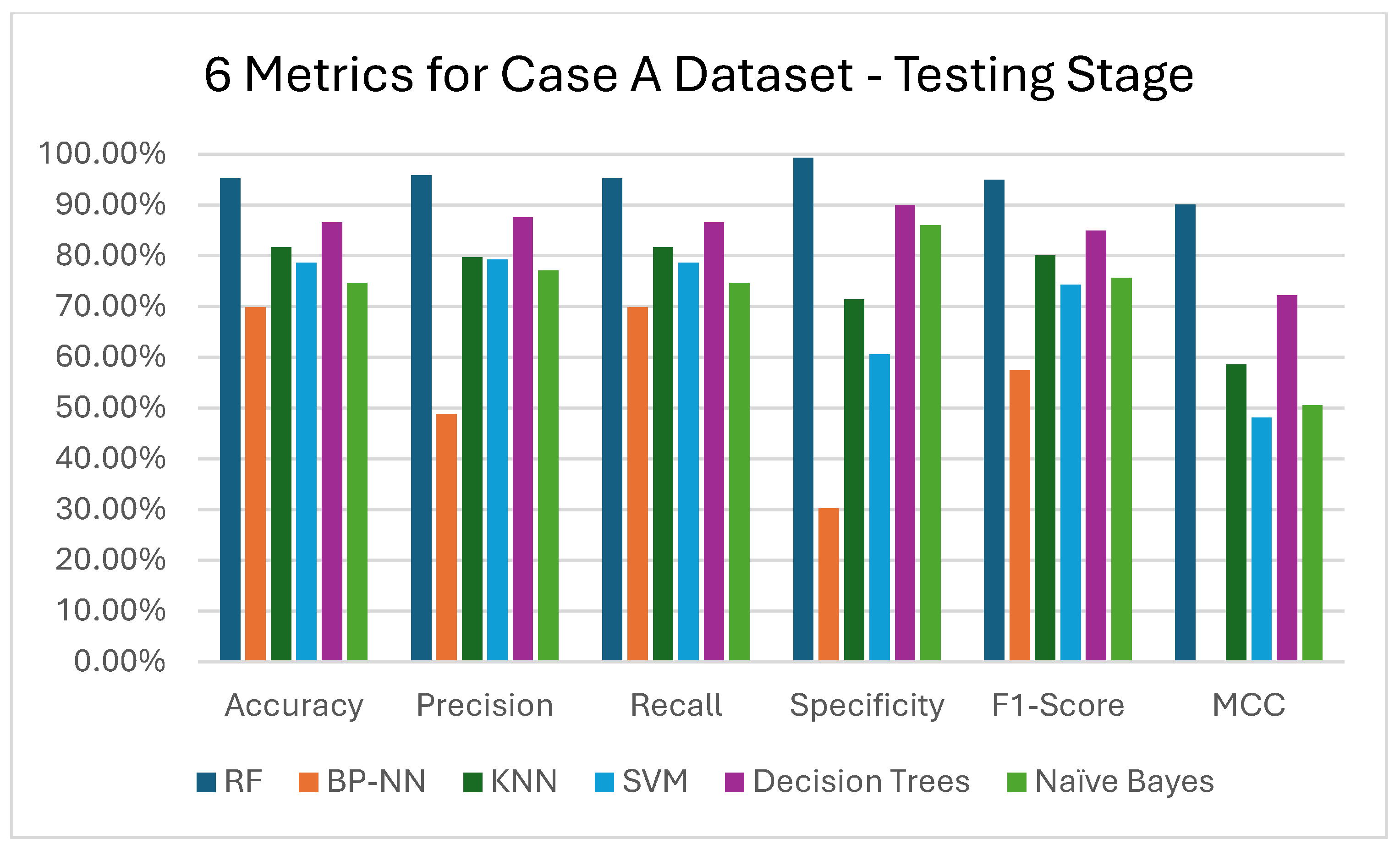
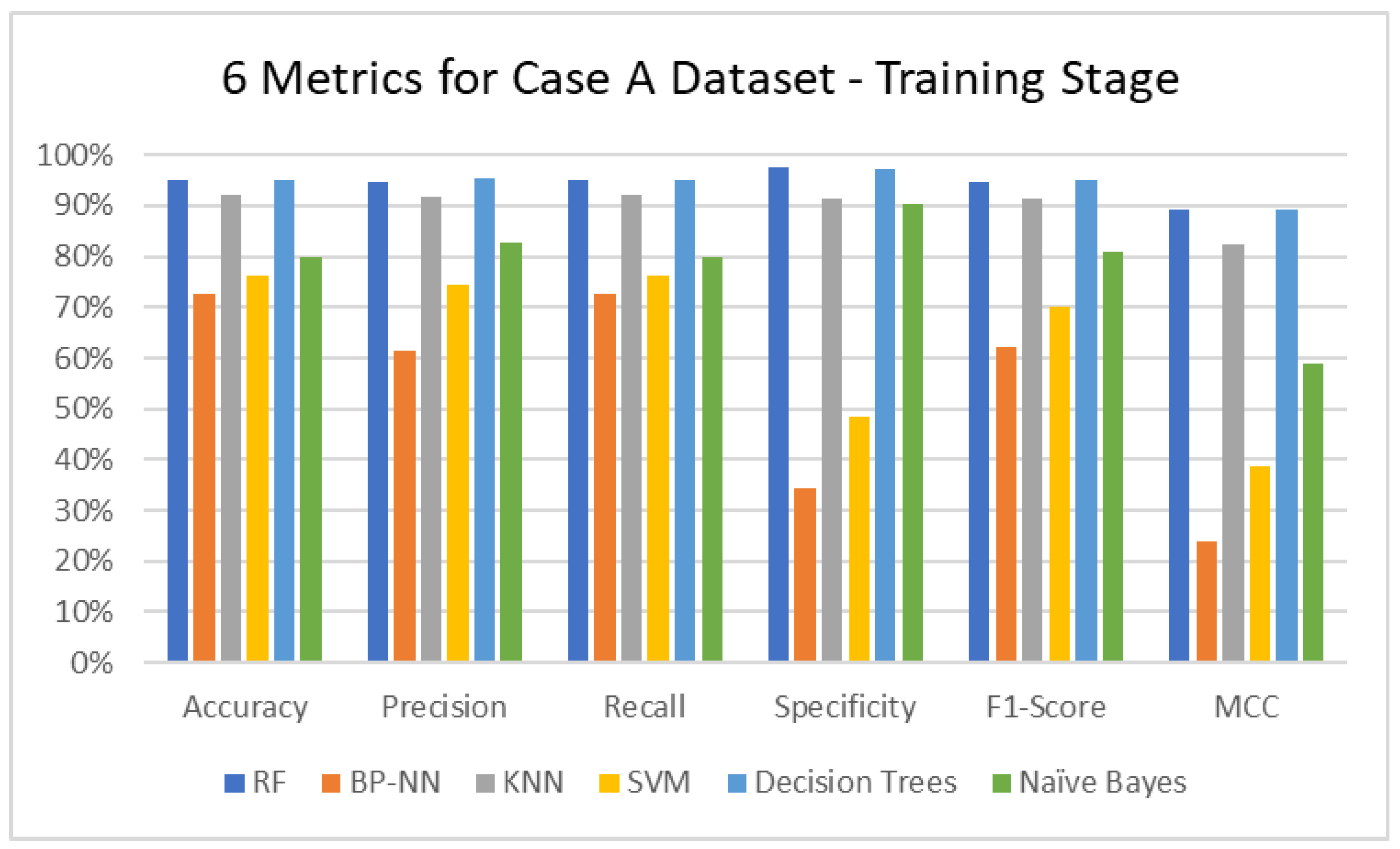
Figure 2 and Figure 3 illustrate the results chart of the six metrics for MLMs on the case A dataset.

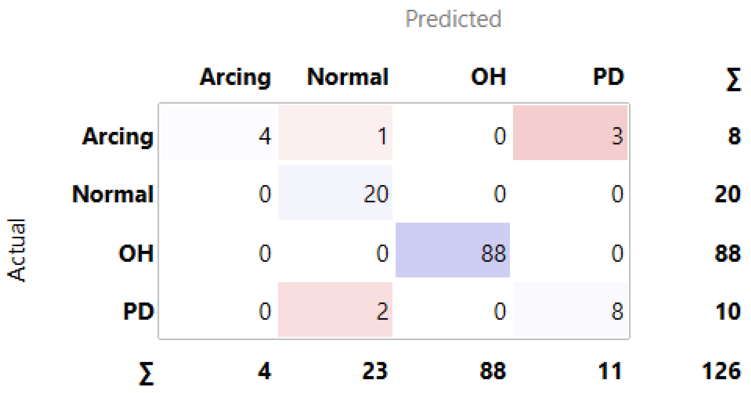
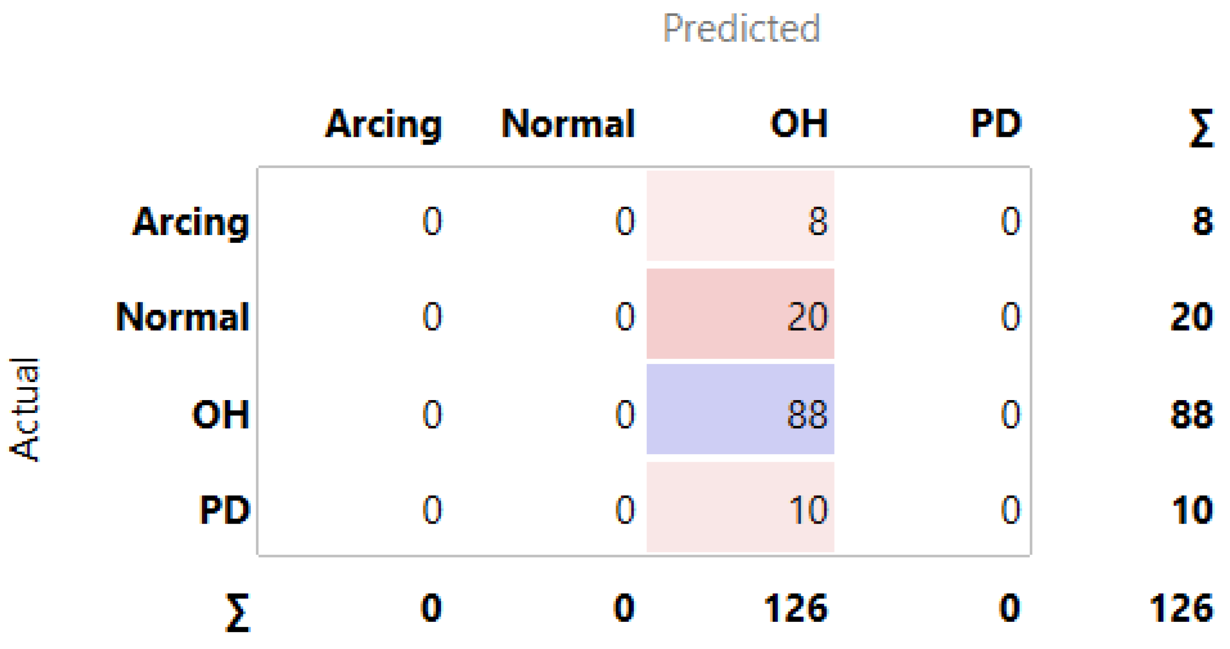
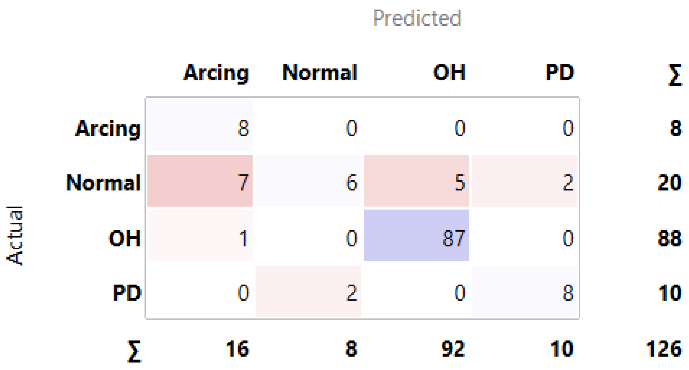
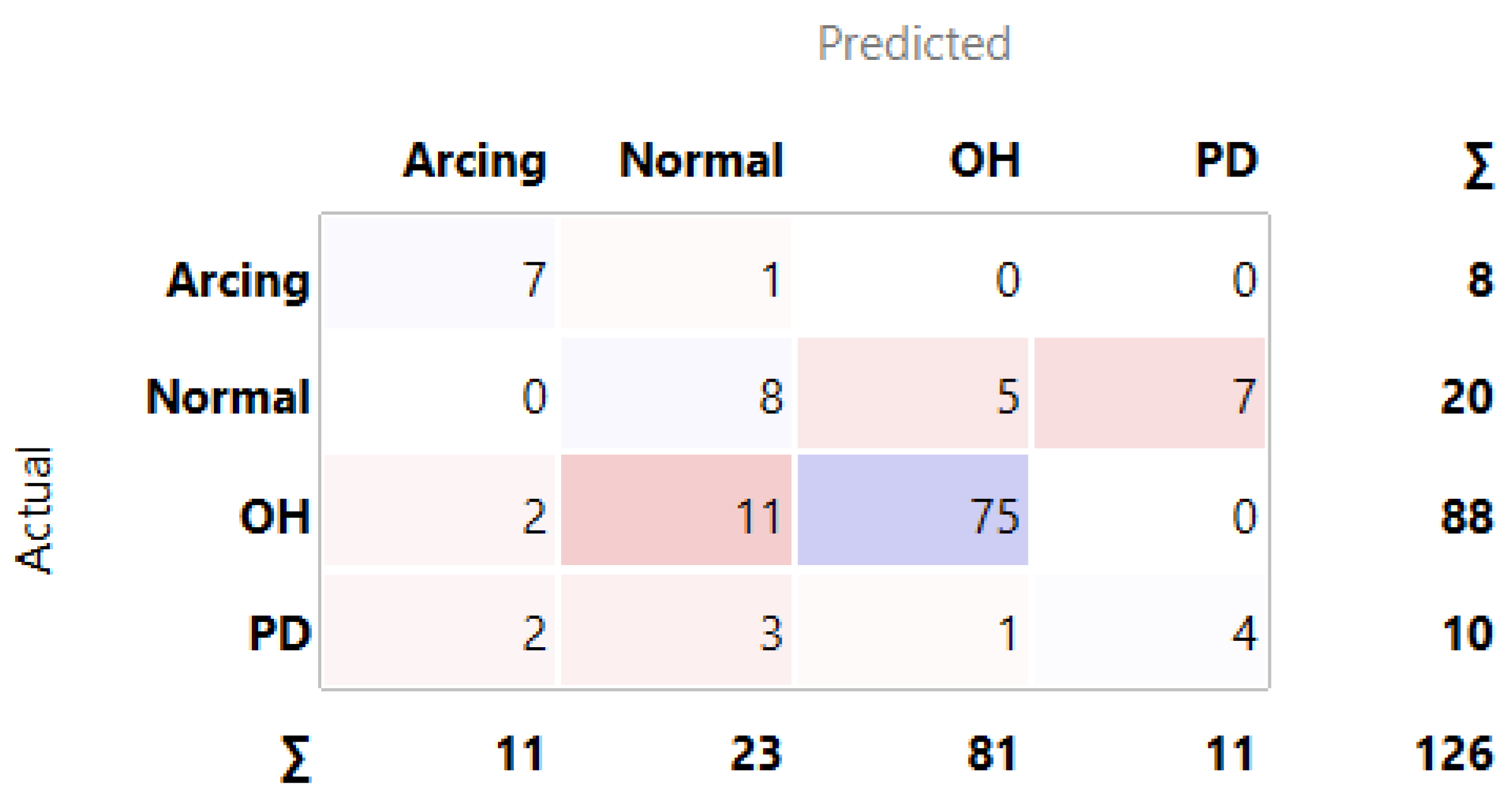
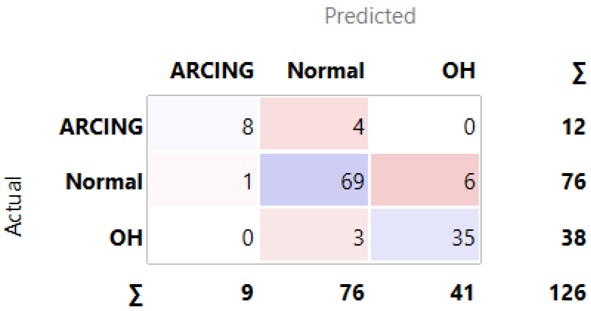
In the case A dataset, which used the three gas percentages, RF obtained the best accuracy in both the training and testing stages (95% and 95.2%, respectively). Additionally, in the other metrics, RF also obtained the best values in both the training and testing stages. The confusion matrices of all six MLMs in the testing stage have been illustrated in Figure 4, Figure 5, Figure 6, Figure 7, Figure 8 and Figure 9 below for the RF, BPNN, KNN, SVM, DT, and NB algorithms, respectively.

As mentioned above, RF obtained the best accuracy. The confusion matrix of RF in Figure 2 shows that the OH fault has the highest accuracy detection with Normal detection.

4.2. Case B

In this case of fault diagnosis with the DRM, the following ratios were used as the dataset: C₂H₆/C₂H₂, C₂H₂/CH₄, C₂H₂/C₂H₄, and CH₄/H₂. The diagnostic performance results of the machine learning classification algorithms are presented in

Table 7. Machine learning methods’ performance evaluation results: case B training.

Method	Accuracy	Precision	Recall	Specificity	F1 Score	MCC
RF	99.8%	99.8%	99.8%	99.8%	99.8%	99.7%
BPNN	49.3%	42%	49.3%	51.5%	33%	7.2%
KNN	92%	92%	92%	96.1%	92%	88.1%
SVM	53.9%	45.1%	53.9%	58.7%	42%	23.6%
Decision Tree	99.2%	99.2%	99.2%	99.7%	99.2%	98.8%
Naive Bayes	87.8%	90.7%	87.7%	96.9%	87.6%	82.9%

and

Table 8. Machine learning methods’ performance evaluation results: case B testing.

Method	Accuracy	Precision	Recall	Specificity	F1 Score	MCC
RF	100%	100%	100%	100%	100%	100%
BPNN	49.2%	24.2%	49.2%	50.8%	32.5%	0%
KNN	89.7%	90%	89.7%	93.7%	89.4%	84.6%
SVM	54.8%	54.1%	54.8%	56.8%	43%	27.2%
Decision Tree	100%	100%	100%	100%	100%	100%
Naive Bayes	93.7%	95%	93.7%	98.9%	93.6%	91%

for training and testing, respectively.

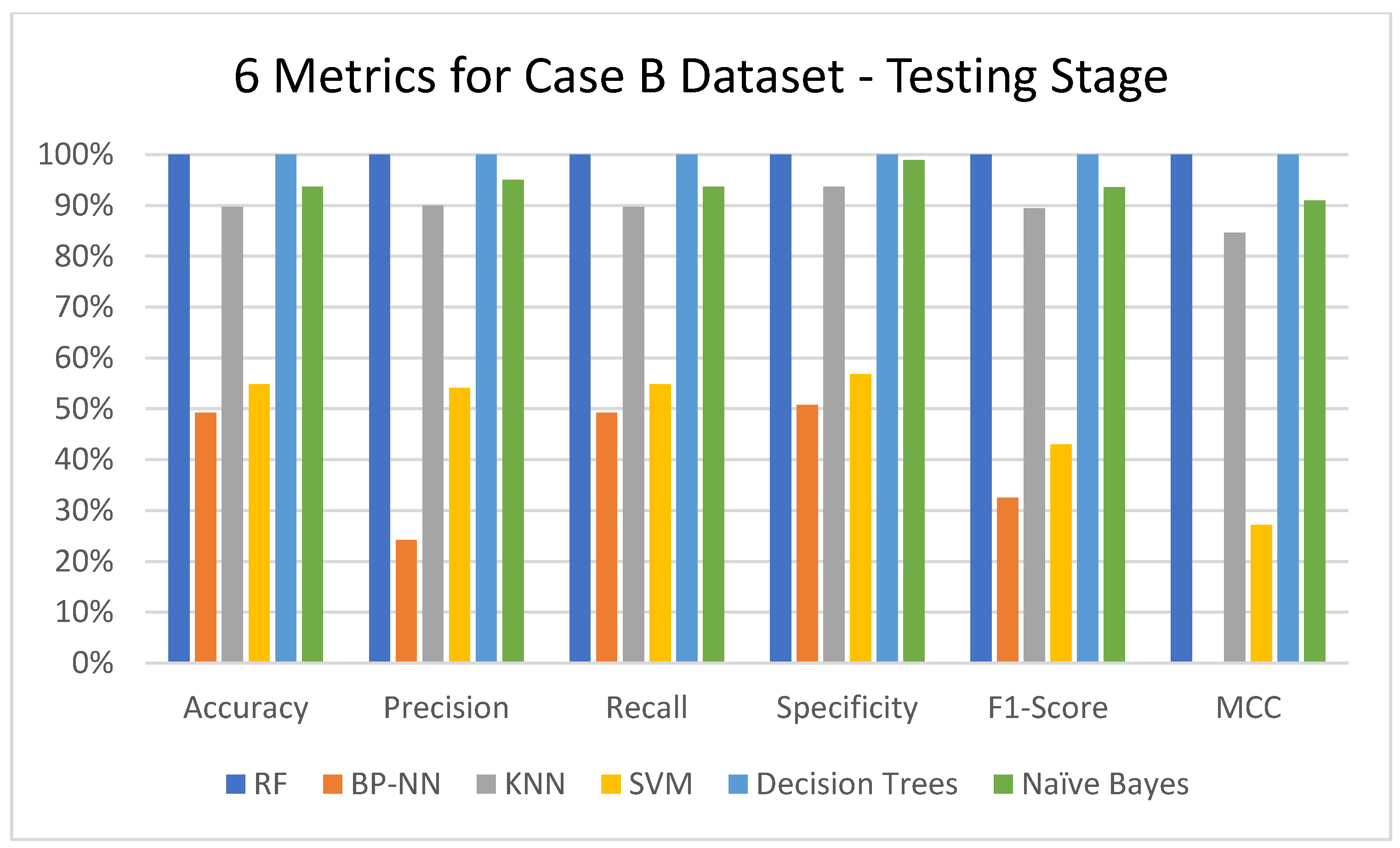
Figure 10 and Figure 11 illustrate the results chart of the six metrics for MLMs on the case B dataset.

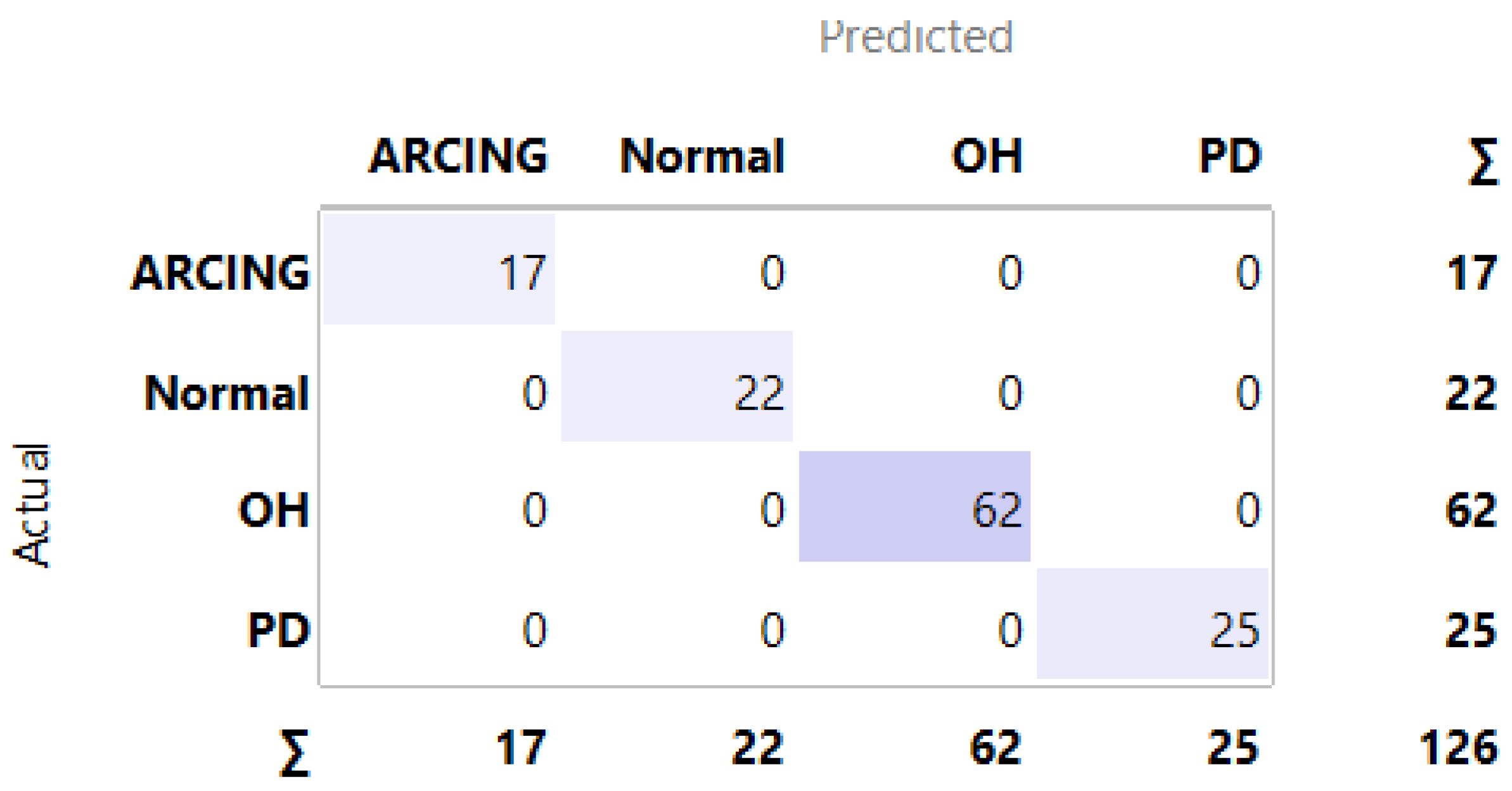
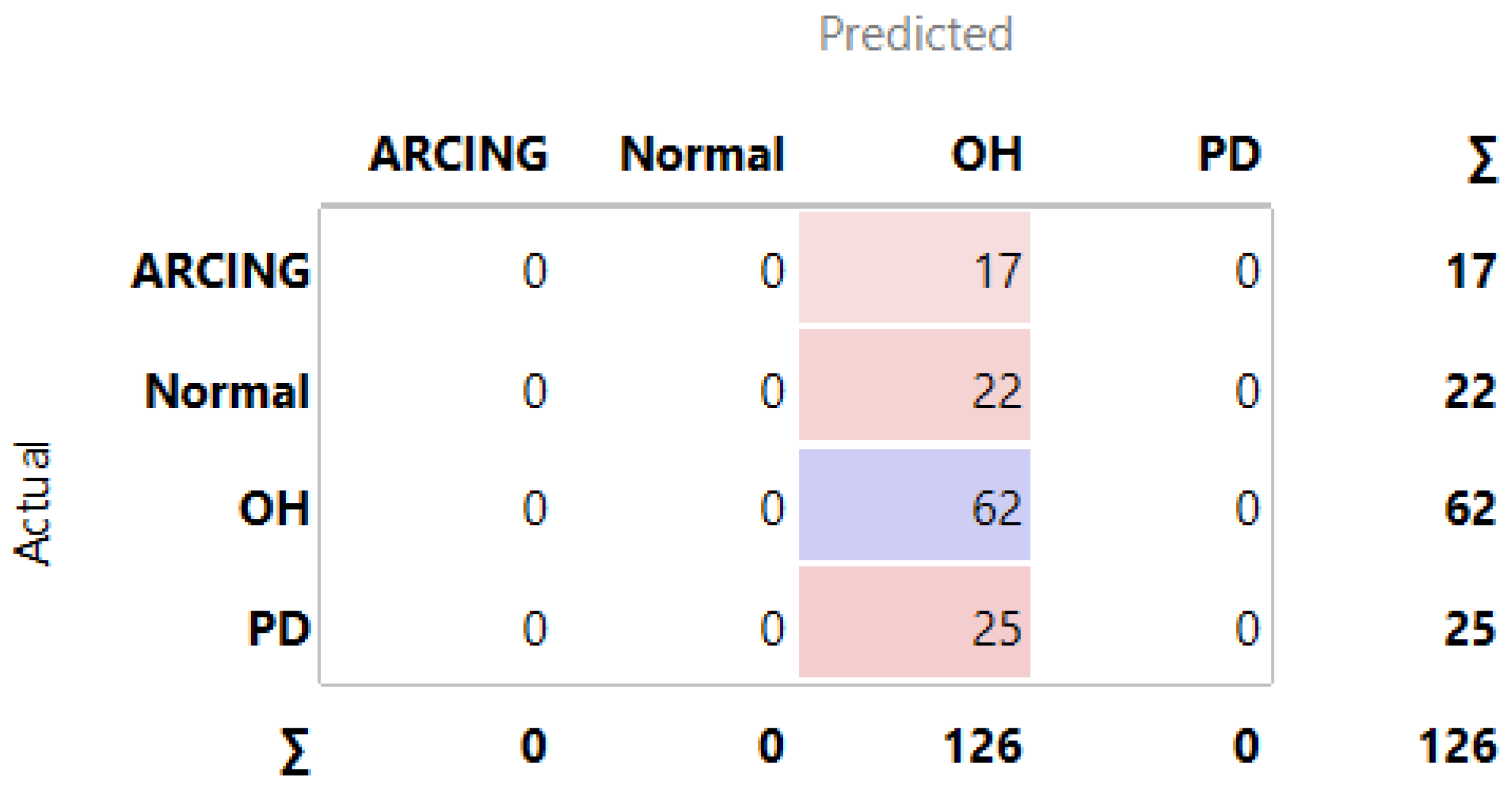
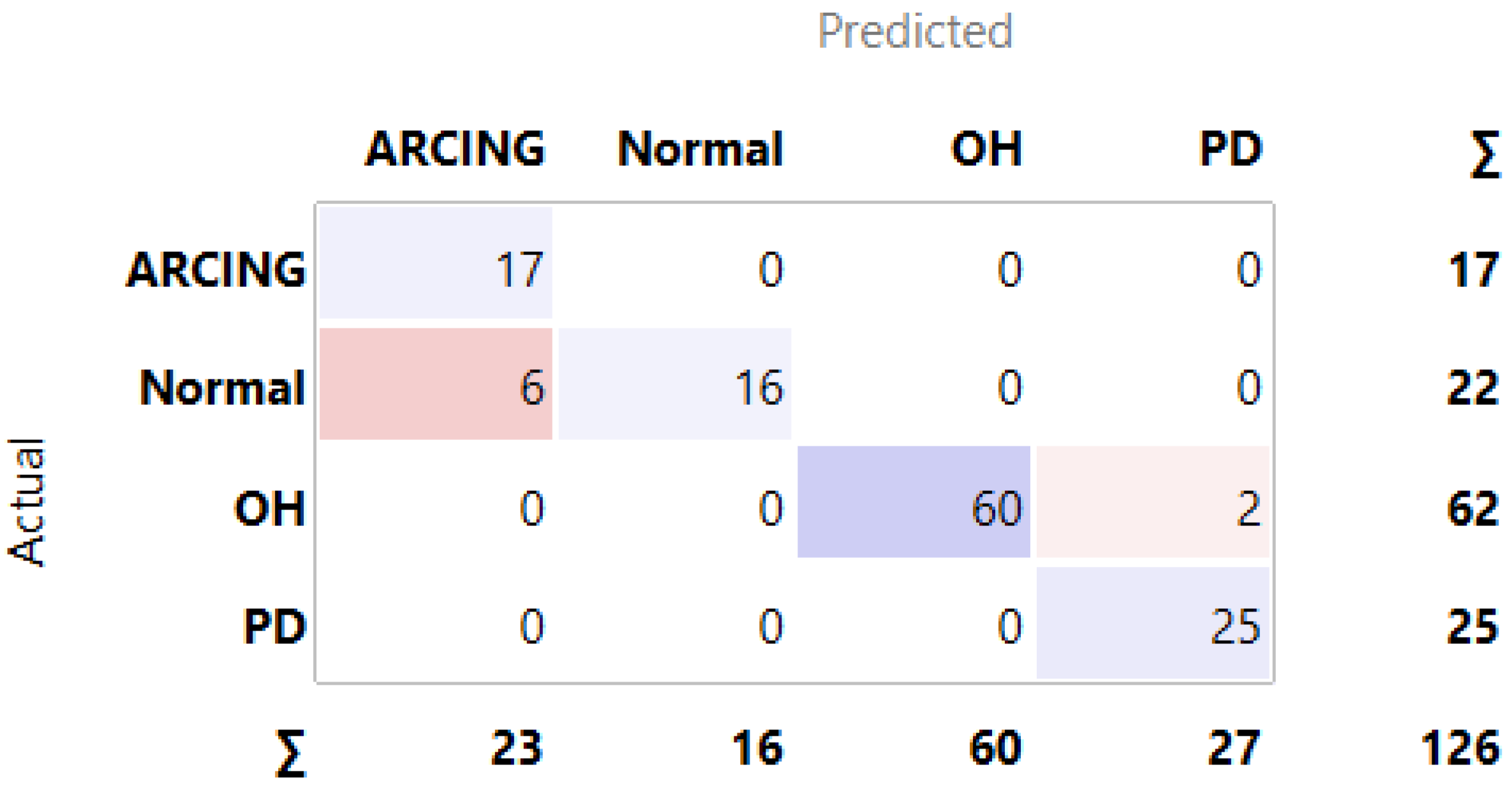
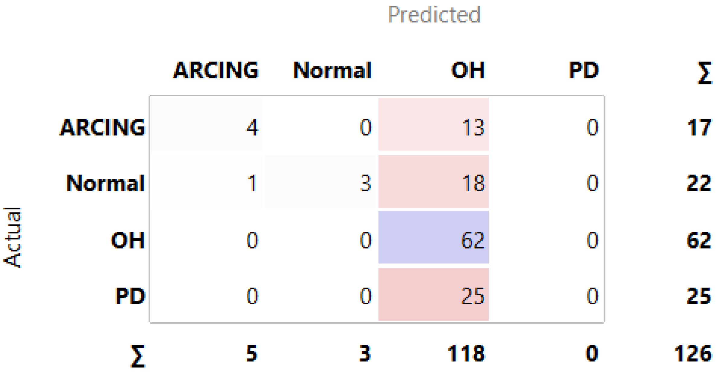
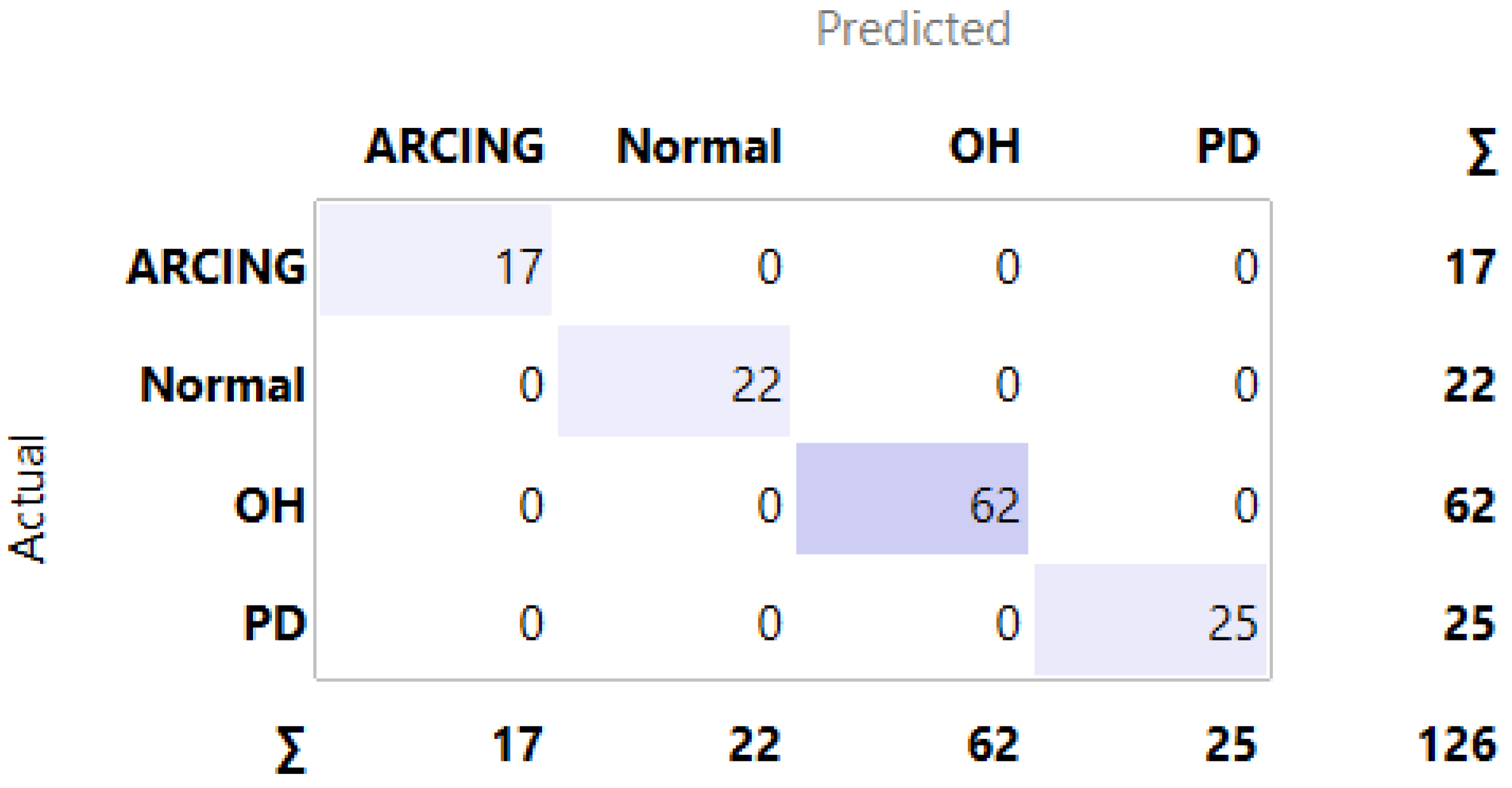
In the case B dataset, which used the three gas percentages, RF obtained the best accuracy in the training stage (99.8%). In the testing stage, RF and DT obtained the best accuracy (100%). The best values for the other metrics were also obtained when using RF and DT in both the training and testing stages. The confusion matrices of all six MLMs in the testing stage are illustrated in Figure 12, Figure 13, Figure 14, Figure 15, Figure 16 and Figure 17 for the RF, BPNN, KNN, SVM, DT, and NB algorithms, respectively.

As we mentioned above, RF and DT obtained the best accuracy. The confusion matrices of RF and DT in Figure 12 and Figure 17 show that all types of faults were detected with 100% accuracy.

4.3. Case C

In this case using the RRM, five gas concentrations obtained with the dissolved gas method were used for dataset input in the classification algorithms. The results for these algorithms are presented in

Table 9. Machine learning methods’ performance evaluation results: case C training.

Method	Accuracy	Precision	Recall	Specificity	F1 Score	MCC
RF	99.4%	99.4%	99.4%	99.4%	99.4%	98.9%
BPNN	60.1%	36.1%	60.1%	39.9%	45.1%	0%
KNN	94%	94%	94%	94.5%	94%	88.9%
SVM	47.3%	58.9%	47.3%	69.2%	43.2%	23.5%
Decision Tree	99.4%	99.4%	99.4%	99.4%	99.4%	98.9%
Naive Bayes	80%	82.5%	80%	87%	80.7%	65.7%

and

Table 10. Machine learning methods’ performance evaluation results: case C testing.

Method	Accuracy	Precision	Recall	Specificity	F1 Score	MCC
RF	99.2%	99.2%	99.2%	98.8%	99.2%	98.5%
BPNN	60.3%	36.4%	60.3%	39.7%	45.4%	0%
KNN	88.9%	89%	88.9%	89.4%	88.7%	79.2%
SVM	31.7%	18.8%	31.7%	60.2%	18%	0%
Decision Tree	99.2%	99.2%	99.2%	98.8%	99.2%	98.5%
Naive Bayes	83.3%	84.2%	83.3%	86.2%	83.5%	69.7%

for training and testing, respectively.

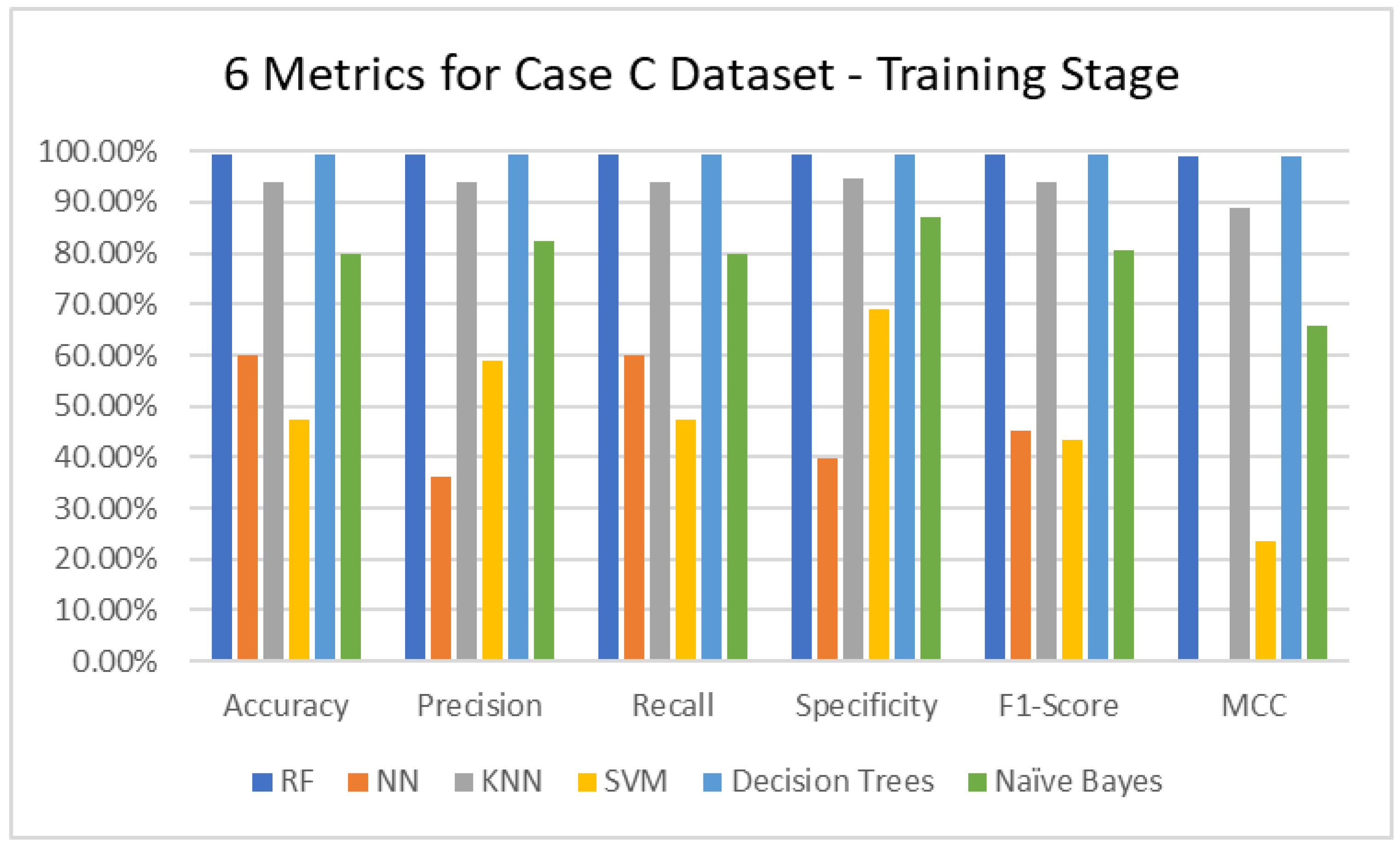
Figure 18 and Figure 19 illustrate the results chart of the six metrics for MLMs on the case C dataset.

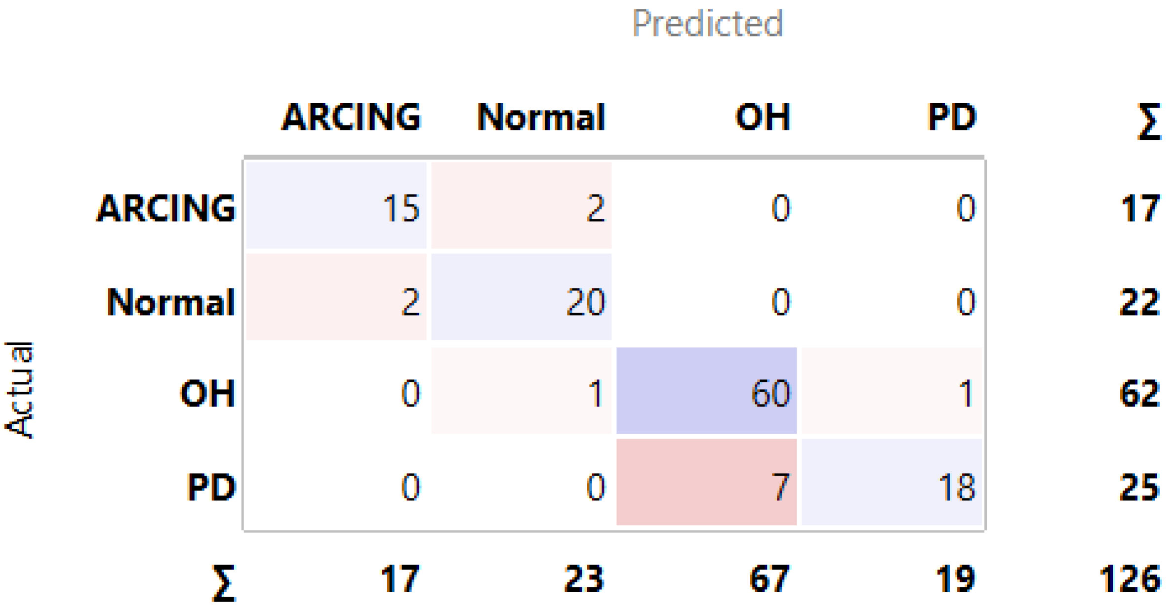
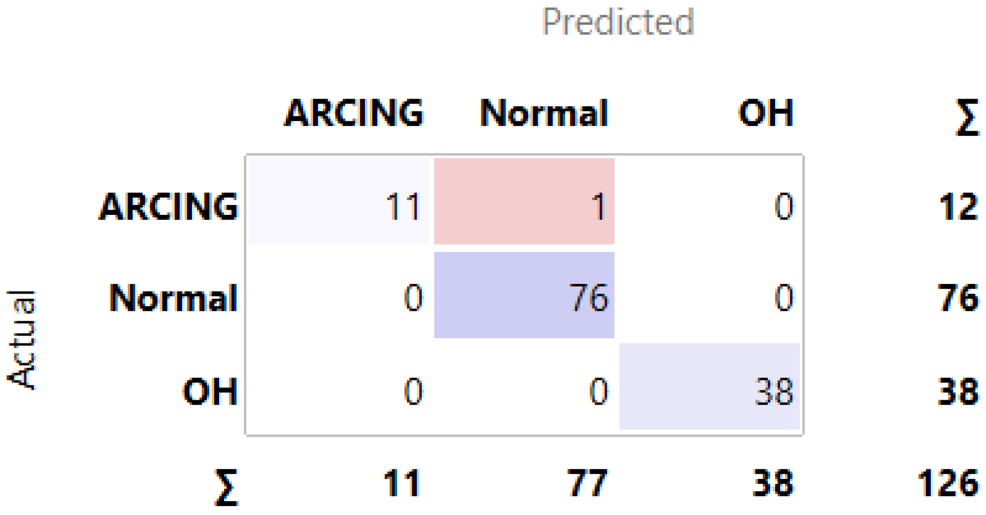
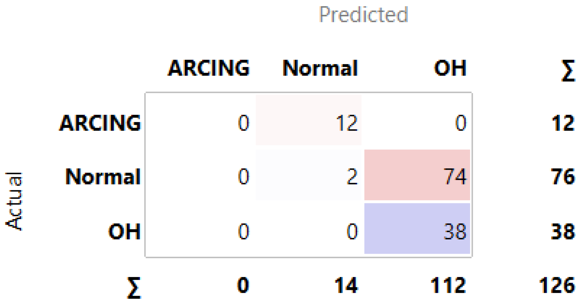
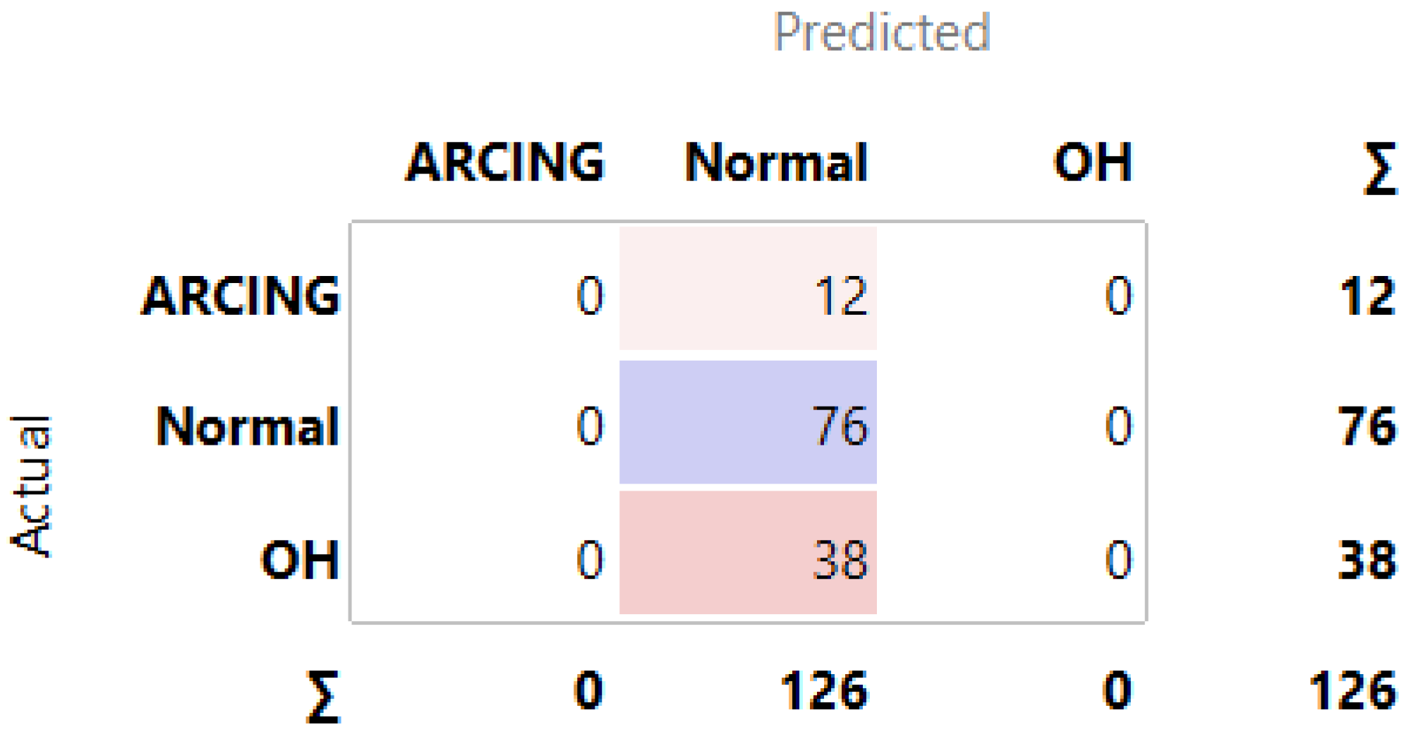
In the case C dataset, which used the three gas percentages, RF and DT obtained the best accuracy in the training stage (99.4%). Further, in the testing stage, RF and DT obtained the best accuracy (99.2%). The best values for the other metrics were obtained when using RF and DT in both the training and testing stages. The confusion matrices of all six MLMs in the testing stage are illustrated in Figure 20, Figure 21, Figure 22, Figure 23, Figure 24 and Figure 25 for the RF, BPNN, KNN, SVM, DT, and NB algorithms, respectively.

As mentioned above, RF and DT obtained the best accuracy. The confusion matrices of RF and DT in Figure 20 and Figure 21 show that the OH fault has a detection accuracy of 100%.

In this paper, gas percentages and gas ratios from conventional methods have been used to compare the data inputs for classification algorithms. The highest results for accuracy, precision, recall, specificity, F1 score, and Matthews correlation coefficient diagnostic were obtained for the three gas percentages used in the DRM, with the RF and DT algorithms performing the best.

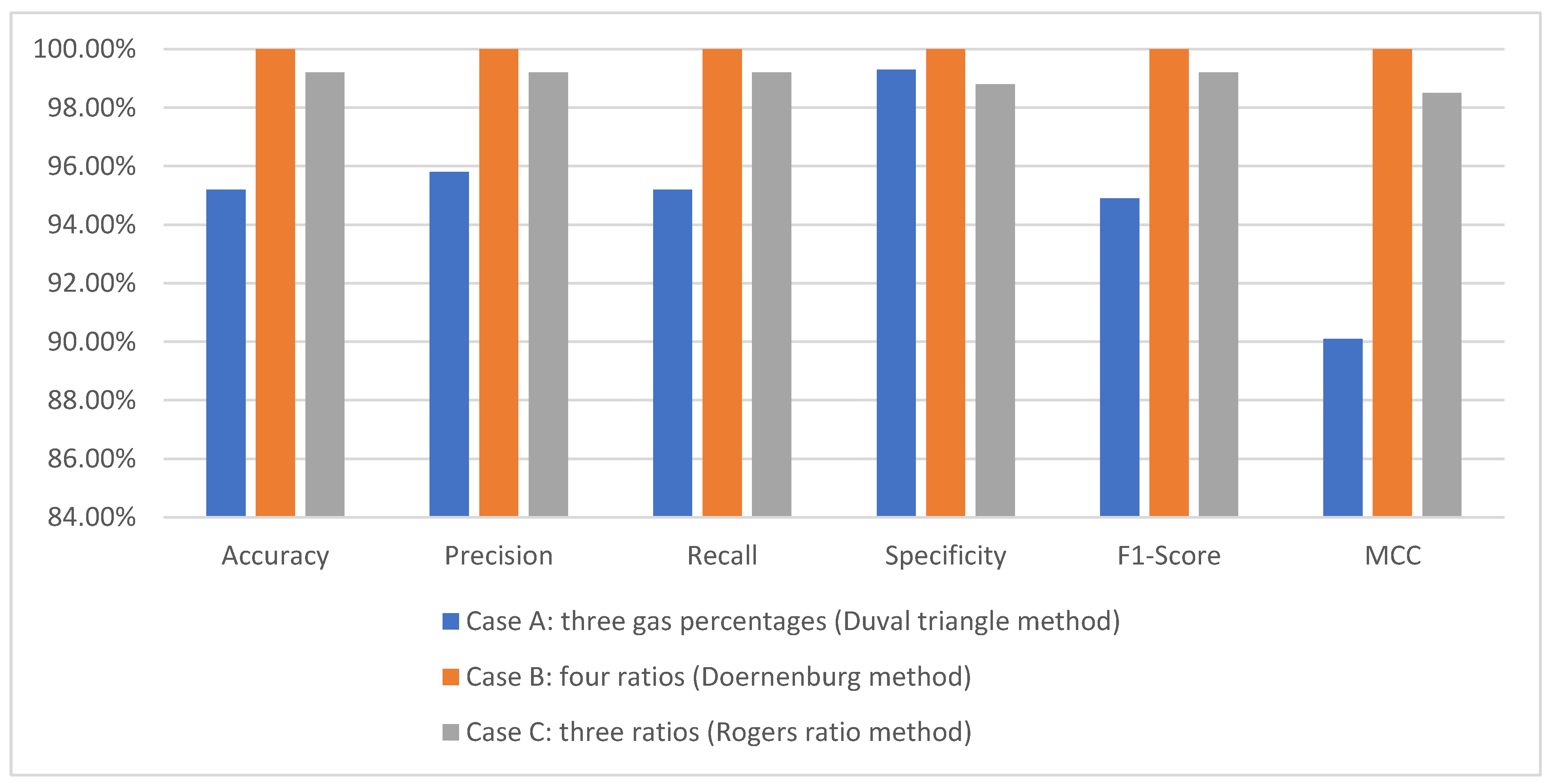
A summary of the best diagnostic results for accuracy, precision, recall, specificity, F1 score, and Matthews correlation coefficient for the different testing datasets is given in

Table 11. Best diagnostic performance results for different dataset cases.

Dataset	Best Algorithm	Metrics
		Accuracy	Precision	Recall	Specificity	F1 Score	MCC
Case A: Three gas percentages (Duval triangle method)	RF	95.2%	95.8%	95.2%	99.3%	94.9%	90.1%
Case B: Four ratios (Doernenburg’s method)	RF and DT	100%	100%	100%	100%	100%	100%
Case C: Three ratios (Rogers ratio method)	RF and DT	99.2%	99.2%	99.2%	98.8%	99.2%	98.5%

.

Figure 26 shows a comparison of the performance evaluation results obtained between the datasets for all types of faults. This figure illustrates that the best results for accuracy, precision, recall, specificity, F1 score, and Matthews correlation coefficient were obtained with the Doernenburg method (four concentrations) and the RF algorithm, with similar resulted obtained (at testing) by the DT algorithm.

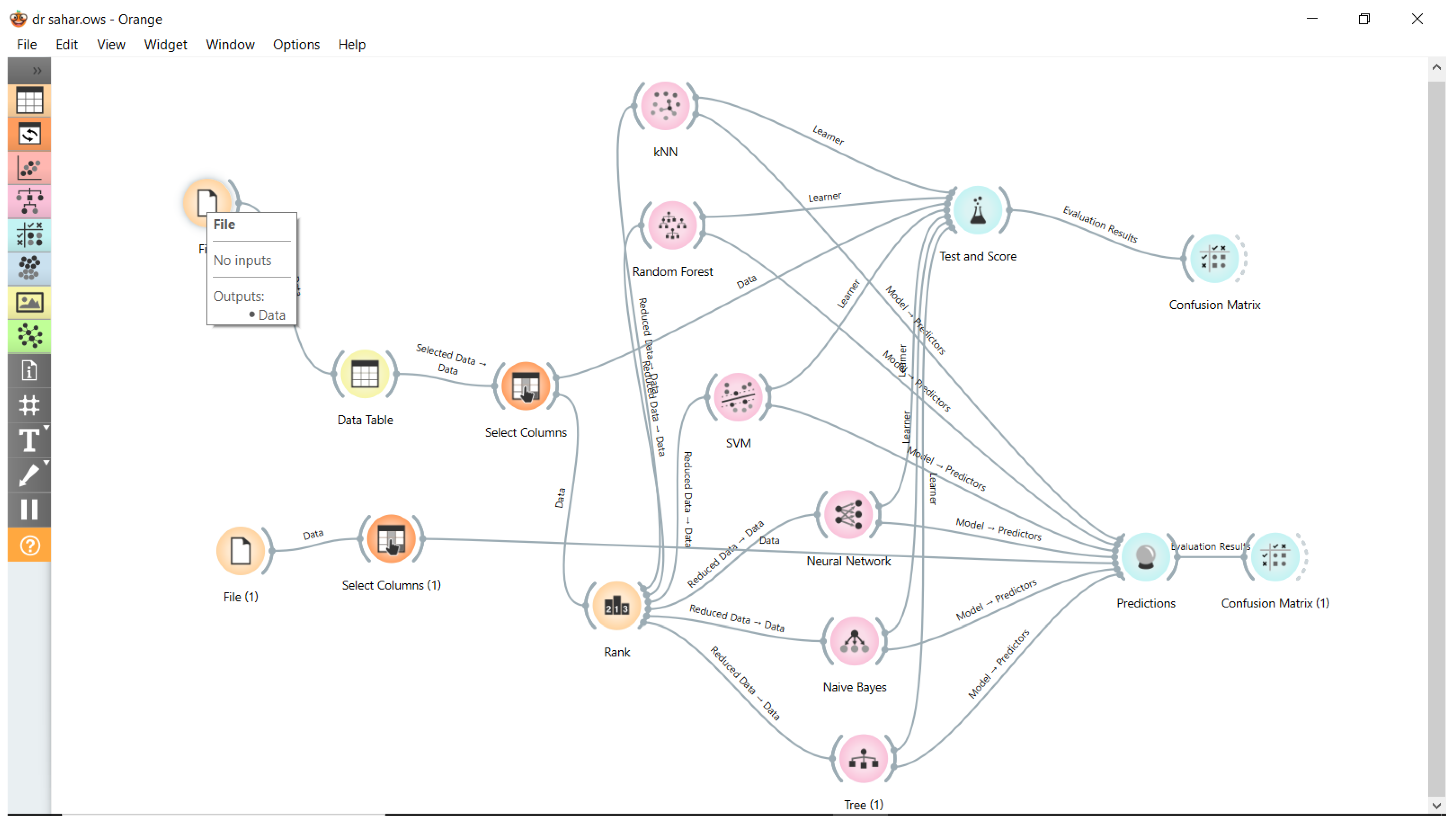
Figure 27 shows the Orange Data Mining details for the DRM dataset as an example of our work. All Orange Data Mining code is available at https://github.com/ahmedtariq71/PowerTransformerCode (accessed on 13 December 2024).

5. Conclusions

In this paper, fault diagnosis for a power transformer was performed using six machine learning classification methods and three dataset transformation techniques, namely DTM, DRM, and RRM. The six classification techniques used were RF, BPNN, KNN, SVM, DT, and NB. The three transformation methods were implemented to enhance the accuracy of fault prediction, as well as other criteria such as the precision, recall, F1 score, specificity, and Matthews correlation coefficient (MCC) of the suggested methods. The dataset transformation methods involved gas percentages and gas ratios.

While the results obtained from the work have been compared, it was noticed that a better diagnostic accuracy, precision, recall, F1 score, and Matthews correlation coefficient (MCC) for all cases were observed with the four gas ratios used in Doernenburg’s method. The utilization of different dataset inputs does not always positively affect the classification performance; for example, it was noticed that the classification performance decreased in case C, which used the Rogers ratio method.

This illustrates that a certain dataset used does not hold the essential information for an algorithm to produce an exact diagnosis. The results show that the dataset content in this work for classification algorithms for training and testing had a great effect on the performance.

The results of RF were the best for the three types of datasets because this method relies on generating a good number of solutions and selects the best among them, which distinguishes it from other methods of machine learning.

References

1. Yang, Z.; Tang, W.H.; Shintemirov, A.; Wu, Q.H. Association Rule Mining-Based Dissolved Gas Analysis for Fault Diagnosis of Power Transformers. IEEE Trans. Syst. Man Cybern. Part C Appl. Rev. 2009, 39, 597–610. [Google Scholar] [CrossRef]
2. Suna, H.-C.; Huanga, Y.-C.; Huang, C.-M. A review of dissolved gas analysis in power transformers. Energy Procedia 2012, 14, 1220–1225. [Google Scholar] [CrossRef]
3. Wani, S.A.; Khan, S.A.; Prashal, G.; Gupta, D. Smart Diagnosis of Incipient Faults Using Dissolved Gas Analysis-Based Fault Interpretation Matrix (FIM). Arab. J. Sci. Eng. 2019, 44, 6977–6985. [Google Scholar] [CrossRef]
4. Zhang, Y.; Chen, H.C.; Du, Y.; Chen, M.; Liang, J.; Li, J.; Fan, X.; Yao, X. Power transformer fault diagnosis considering data imbalance and data set fusion. High Volt. 2021, 6, 543–554. [Google Scholar] [CrossRef]
5. Senoussaoui, M.E.A. Contribution Des Techniques Intelligences Au Diagnostic Industrial Des Transformations De Puissance. Ph.D. Thesis, Université Djillali Liabbes De Sidi Bel Abbes, Sidi Bel Abbes, Algeria, 2019. [Google Scholar]
6. Bustamante, S.; Manana, M.; Arroyo, A.; Castro, P.; Laso, A.; Martinez, R. Dissolved Gas Analysis Equipment for Online Monitoring of Transformer Oil: A Review. Sensors 2018, 19, 4057. [Google Scholar] [CrossRef]
7. IEEE. IEEE Guide for the Interpretation of Gases Generated in Mineral Oil-Immersed Transformers IEEE Std C57.104TM; IEEE Power and Energy Society: Piscataway, NJ, USA, 2019. [Google Scholar]
8. Xie, H.; Chen, J.; Zhang, P.; Zhang, F.; Meng, X.; Cheng, J. Knowledge Acquisition for Transformer Condition Assessment Using Synthetic Minority Over-sampling Technique and Decision Tree Algorithm. In Proceedings of the 2019 IEEE Innovative Smart Grid Technologies—Asia (ISGT Asia), Chengdu, China, 21–24 May 2019; pp. 4186–4191. [Google Scholar]
9. Wu, X.; Kumar, V.; Qinlan, J.R.; Ghosh, J.; Yang, Q.; Motoda, H.; Mclachlan, G.J.; Ng, A.; Liu, B.; Yu, P.S.; et al. Top 10 Algorithms in Data Mining. Knowl. Inf. Syst. 2008, 14, 1–37. [Google Scholar] [CrossRef]
10. Odongo, G.; Musabe, R.; Hanyurwimfura, D. A Multinomial DGA Classifier for Incipient Fault Detection in Oil-Impregnated Power Transformers. Algorithms 2021, 14, 128. [Google Scholar] [CrossRef]
11. Bacha, K.; Souahlia, S.; Gossa, M. Power transformer fault diagnosis based on dissolved gas analysis by support vector machine. Electr. Power Syst. Res. 2012, 83, 73–79. [Google Scholar] [CrossRef]
12. Prasojo, R.A.; Gumilang, H.; Suwarno; Maulidevi, N.U.; Soedjarno, B.A. A fuzzy logic model for power transformer faults’ severity determination based on gas level, gas rate, and dissolved gas analysis interpretation. Energies 2020, 13, 1009. [Google Scholar] [CrossRef]
13. Liu, Y.; Song, B.; Wang, L.; Gao, J.; Xu, R. Power transformer fault diagnosis based on dissolved gas analysis by correlation coefficient-DBSCAN. Appl. Sci. 2020, 10, 4440. [Google Scholar] [CrossRef]
14. Abu-Siada, A. Improved consistent interpretation approach of Fault Type within power transformers using dissolved gas analysis and Gene expression programming. Energies 2019, 12, 730. [Google Scholar] [CrossRef]
15. Shah, A.M.; Bhalja, B.R. Fault discrimination scheme for power transformer using random forest technique. IET Gener. Transm. Distrib. 2016, 10, 1431–1439. [Google Scholar] [CrossRef]
16. Badawi, M.; Ibrahim, S.A.; Mansour, D.-E.A.; El-Faraskoury, A.A.; Ward, S.A.; Mahmoud, K.; Lehtonen, M.; Darwish, M.M.F. Reliable estimation for health index of transformer oil based on novel combined predictive maintenance techniques. IEEE Access 2022, 10, 25954–25972. [Google Scholar] [CrossRef]
17. Kartojo, I.H.; Wang, Y.-B.; Zhang, G.-J. Suwarno Partial Discharge Defect Recognition in Power Transformer Using Random Forest. In Proceedings of the 2019 IEEE 20th International Conference on Dielectric Liquids (ICDL), Roma, Italy, 23–27 June 2019; pp. 1–4. [Google Scholar]
18. N’Cho, J. Développement De Nouvelles Méthodes De Diagnostic Et De Régénération Des Huiles Pour Transformateurs De Puis-Sance. Ph.D. Thesis, Ecole Centrale de Lyon, Écully, France, 2011. [Google Scholar]
19. Abidin, Z.; Shukri, M.; Rashid, H.A.; Marzuki, K.; Rohani, A.M.; Razak, A.; Afifi, M.; Mustaffa; Suryani; Aisyah, I.S.H.; et al. Design of a fault diagnostic engine for power transformer using data mining. Fac. Electr. Eng. 2007, Unpublished. Available online: https://core.ac.uk/outputs/11781963/ (accessed on 13 December 2024).
20. Illias, H.A.; Liang, W.Z. Identification of transformer fault based on dissolved gas analysis using hybrid support vector ma-chine-modified evolutionary particle swarm optimization. PLoS ONE 2018, 13, e0191366. [Google Scholar] [CrossRef]
21. Mansour, D.-E.A. Development of a new graphical technique for dissolved gas analysis in power transformers based on the five combustible gases. IEEE Trans. Dielectr. Electr. Insul. 2015, 22, 2507–2512. [Google Scholar] [CrossRef]
22. Gouda, O.E.; El-Hoshy, S.H.; Tamaly, H.H. Condition assessment of power transformers based on dissolved gas analysis. IET Gener. Transm. Distrib. 2019, 13, 2299–2310. [Google Scholar] [CrossRef]
23. Géron, A. Hands-On Machine Learning with Scikit-Learn and Tensorflow Concepts; O’Reilly Publishing: Sebastopol, CA, USA, 2017. [Google Scholar]
24. Bernard, S.; Adam, S.; Heutte, L. Using Random Forests for Handwritten Digit Recognition. In Proceedings of the Ninth International Conference on Document Analysis and Recognition (ICDAR 2007), Curitiba, Brazil, 23–26 September 2007; pp. 1043–1047. [Google Scholar]
25. Gilles Louppe. Understanding Random Forests: From Theory to Practice. Available online: https://arxiv.org/pdf/1407.7502.pdf (accessed on 13 December 2024).
26. Ghoneim, S.S.M.; Taha, I.B.M.; Elkalashy, N.I. Integrated ANN-based proactive fault diagnostic scheme for power transformers using dissolved gas analysis. IEEE Trans. Dielectr. Electr. Insul. 2016, 23, 1838–1845. [Google Scholar] [CrossRef]
27. Benmahamed, Y.; Teguar, M.; Boubakeur, A. Diagnosis of Power Transformer Oil Using PSO-SVM and KNN Classifiers. In Proceedings of the International Conference on Electrical Sciences and Technologies in Maghreb (CISTEM), Algiers, Algeria, 28–31 October 2018; pp. 1–4. [Google Scholar]
28. Demirci, M.; Gozde, H.; Taplamacioglu, M.C. Comparative Dissolved Gas Analysis with Machine Learning and Traditional Methods. In Proceedings of the 2021 3rd International Congress on Human-Computer Interaction, Optimization and Robotic Applications (HORA), Ankara, Turkey, 11–13 June 2021; pp. 1–6. [Google Scholar]
29. Alqudsi, A.; El-Hag, A. Application of machine learning in transformer health index prediction. Energies 2019, 12, 2694. [Google Scholar] [CrossRef]
30. Yeh, D.-Y.; Cheng, C.-H.; Hsiao, S.-C. Classification knowledge discovery in mold tooling test using decision tree algorithm. J. Intell. Manuf. 2011, 22, 585–595. [Google Scholar] [CrossRef]
31. Jiang, L.; Cai, Z.; Zhang, H.; Wang, D. Naive Bayes text classifiers: A locally weighted learning approach. J. Exp. Theor. Artif. Intell. 2013, 25, 273–286. [Google Scholar] [CrossRef]
32. Abu-Siada, A.; Hmood, S. A new fuzzy logic approach to identify power transformer criticality using dissolved gas-in-oil analysis. Int. J. Electr. Power Energy Syst. 2015, 67, 401–408. [Google Scholar] [CrossRef]
33. Sokolova, M.; Lapalme, G. A systematic analysis of performance measures for classification tasks. Inf. Process. Manag. 2009, 45, 427–437. [Google Scholar] [CrossRef]
Figure 1. Flow chart of the methodology of the DGA technique.
Applsci 15 00118 g001
Figure 2. Chart of 6 metrics for case A dataset—training stage.
Applsci 15 00118 g002
Figure 3. Chart of 6 metrics for case A dataset—testing stage.
Applsci 15 00118 g003
Figure 4. Confusion matrix of case A dataset for RF—testing stage.
Applsci 15 00118 g004
Figure 5. Confusion matrix of case A dataset for BPNN—testing stage.
Applsci 15 00118 g005
Figure 6. Confusion matrix of case A dataset for KNN—testing stage.
Applsci 15 00118 g006
Figure 7. Confusion matrix of case A dataset for SVM—testing stage.
Applsci 15 00118 g007
Figure 8. Confusion matrix of case A dataset for DT—testing stage.
Applsci 15 00118 g008
Figure 9. Confusion matrix of case A dataset for NB—testing stage.
Applsci 15 00118 g009
Figure 10. Chart of 6 metrics for case B dataset—training stage.
Applsci 15 00118 g010
Figure 11. Chart of 6 metrics for case B dataset—testing stage.
Applsci 15 00118 g011
Figure 12. Confusion matrix of case B dataset for RF—testing stage.
Applsci 15 00118 g012
Figure 13. Confusion matrix of case B dataset for KNN—testing stage.
Applsci 15 00118 g013
Figure 14. Confusion matrix of case B dataset for BPNN—testing stage.
Applsci 15 00118 g014
Figure 15. Confusion matrix of case B dataset for NB—testing stage.
Applsci 15 00118 g015
Figure 16. Confusion matrix of case B dataset for SVM—testing stage.
Applsci 15 00118 g016
Figure 17. Confusion matrix of case B dataset for DT—testing stage.
Applsci 15 00118 g017
Figure 18. Chart of 6 metrics for case C dataset—training stage.
Applsci 15 00118 g018
Figure 19. Chart of 6 metrics for case C dataset—testing stage.
Applsci 15 00118 g019
Figure 20. Confusion matrix of case C dataset for RF—testing stage.
Applsci 15 00118 g020
Figure 21. Confusion matrix of case C dataset for DT—testing stage.
Applsci 15 00118 g021
Figure 22. Confusion matrix of case C dataset for SVM—testing stage.
Applsci 15 00118 g022
Figure 23. Confusion matrix of case C dataset for NB—testing stage.
Applsci 15 00118 g023
Figure 24. Confusion matrix of case C dataset for BPNN—testing stage.
Applsci 15 00118 g024
Figure 25. Confusion matrix of case C dataset for KNN—testing stage.
Applsci 15 00118 g025
Figure 26. Diagnostic performance metrics depending on the dataset (test dataset) for the classification algorithm.
Applsci 15 00118 g026
Figure 27. Orange Data Mining user interface for our work.
Applsci 15 00118 g027