An Analysis of the Kinematics and Dynamics Performance of a New Type of Three-Pronged Sliding Universal Coupling

Abstract

The three-pronged sliding universal coupling is a new kind of three-pronged coupling. The purpose of this study is to demonstrate that, compared with a traditional unequal angular velocity universal coupling (such as the Hooke universal coupling), the universal coupling has the superior characteristics of constant angular speed transmission, simple structure and strong transmission capacity by performing kinematic and dynamic analysis of the new three-pronged sliding constant angular velocity universal coupling. It provides a broad prospect for applications in automotive and other fields. To study its kinematic and dynamic characteristics, directional cosine matrices are utilized as tools to analyze the coordinate systems by establishing simplified geometric models and corresponding motions. Through the analysis of the motions of the input and output shafts and employing the method of single-force element, a set of equilibrium equations for the forces acting on the output shaft and the input shaft are formulated for solution analysis. The research indicates that during the rotation process, there exists a small angular difference between the input shaft and the intermediate shaft, demonstrating the quasi-constant angular velocity characteristics of the new tripod sliding universal coupling. The curves of the forces and force moment acting on each component of the coupling approximate sinusoidal curves. The optimal operating angle range for the new tripod universal coupling is at angle $\beta \le {25}^{°}$, during which the system exhibits good transmission and mechanical performance. It can be widely used in the automobile industry, tie steel industry and other occasions that require angular transmission. It is especially used in high-speed operation and large transmission capacity.

1. Introduction

Couplings are commonly used mechanical transmission components, primarily employed to connect two shafts or for connecting a shaft with other rotating components in various mechanisms. Their purpose is to enable the synchronized rotation of these shafts and facilitate the transmission of motion and torque [1,2,3]. Among them, universal coupling can be applied in situations where there is a significant angular deviation between two shafts, and they can continue to be used even when the angle changes [4,5,6]. Common universal coupling can be classified into three forms based on their motion characteristics: non-constant velocity universal coupling, quasi-constant velocity universal coupling, and constant velocity universal coupling [7,8].

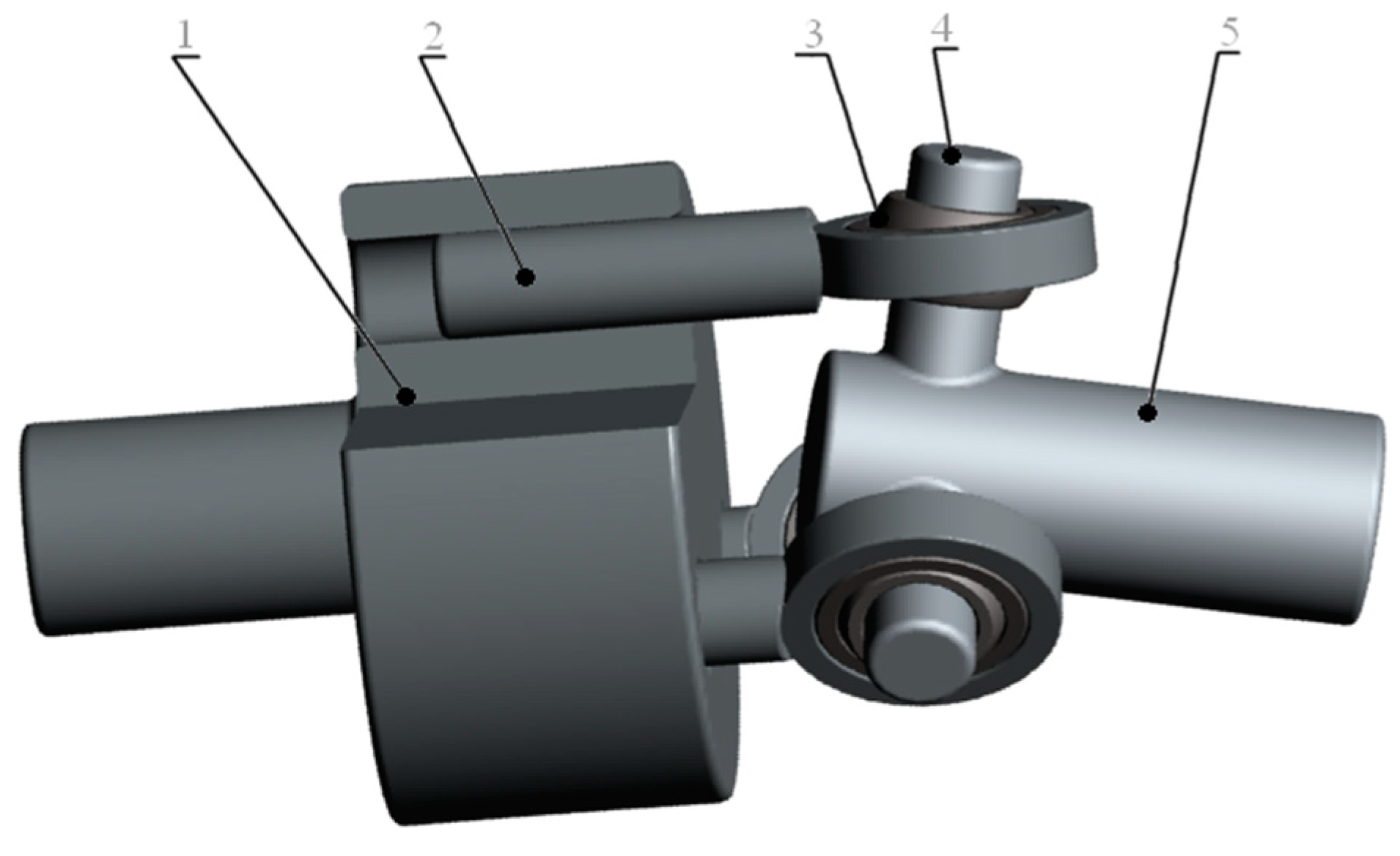
The novel three-pronged sliding universal coupling is a new type of three-pronged coupler invented by our research team [9,10,11], as shown in Figure 1. It mainly consists of a three-pronged sleeve, three sliding pin rods, three inner bearings, and three-pronged itself. Among them, the inner bearing can rotate relatively freely, forming a spherical pair; the sliding pin rod can slide relative to the three-pronged sleeve hole, and is connected to the inner bearing. Compared to traditional three-pronged roller-type couplers, the three-pronged sliding universal coupling uses three sliding pin rods instead of three spherical or cylindrical rollers. This design allows it to transmit larger force moment. Additionally, its structure is simpler, and it comes with advantages such as easy installation, low manufacturing cost, and high transmission efficiency. It can be widely applied in situations requiring heavy torque and heavy loads. By using three sliding pin rods instead of three spherical or cylindrical rollers, the three-pronged sliding universal coupling improves upon the original three-pronged roller-type coupler, which suffered from high contact stress and significant wear due to small contact areas.

This new type of three-pronged sliding universal coupling can be widely used in transmission systems, especially in the automotive industry, with broad prospects for application [12]. Therefore, conducting kinematic and dynamic performance analysis on it is of significant importance, paving the way for further applications in various fields. To achieve a precise analysis of the coupling, it is necessary to clearly define the composition of the coupling before conducting the relevant research. Based on this, we established the motion equations for the three-pronged universal coupling [13]. To understand the motion characteristics of universal couplings and further clarify the motion laws of this device, we designed an analysis method specifically for this device, focusing on the three-pronged universal coupling as the research object [14]. This article utilizes the direction cosine matrix to analyze the motion of the input and output shafts, studying the effects of the angle between the axes of the input and output shafts and the rotational frequency of the coupler on the motion of the sliding pin rod within the triple-rod sleeve holes. Building upon this motion analysis, the single force method is employed [15,16,17] to establish the force equilibrium equations for the output shaft and the input end shaft, followed by solving and analyzing these equations to delve into the dynamic behavior of the input and output shafts. In the dynamic analysis, the use of the single force method bypasses the need for complex solving processes. This method is a straightforward and intuitive approach to force analysis, where the focus lies not on simultaneously determining all constraint forces, but rather on initially calculating the constraint forces within a specific motion pair. Subsequently, the equilibrium equations for the remaining motion pairs are solved individually, component by component. The study of the three-pronged slip universal coupling was mainly carried out in the field of synchronicity and motion law. This research is mainly to establish a kinematic model and dynamic model that can guide the development of a new type of constant angular velocity universal coupling structure, and analyze the kinematics and dynamic characteristics of the new structure, which are of great significance to guide the application of a new type of three-pronged universal coupling. Most of the previous studies carried out by our group focused on the motion trajectory simulation of the components of the three-pronged sliding universal coupling (such as the center point slide bar, etc.), but this study is to establish a guiding model and systematically analyze the model.

In the introduction, the synchronization of the three-pronged sliding universal coupling was verified by the synchronization experiment under different rotation angles. The experimental results show that the universal coupling can achieve the effect of accurate angular velocity rotation. In the case of a rotation angle of less than ${25}^{°}$, the error is very small, and does not affect the engineering application, and can be applied on the occasion that requires the use of equiangular speed transmission universal coupling. The error law of the experiment has an important reference role for the analysis of mechanical properties in this paper. After many experimental verifications, it is proved that the three-pronged sliding cardan shaft has the characteristics of stable transmission capacity in a straight line in the range of commonly used corner ${25}^{°}$. The transmission capacity of the traditional coupling decreases in a curved state, and the decreasing speed is significantly accelerated, resulting in a significant decrease in the transmission capacity. When the rotation angle is less than ${25}^{°}$, the three-pronged sliding universal coupling has the advantage of improving the transmission capacity and, thus, improving the transmission efficiency, which has become an important advantage in the promotion and application.

2. Establishment of Motion, Force Diagram, and Coordinate System

The coordinate system, as illustrated in Figure 2 and Figure 3 [16], is employed: Two fixed coordinate systems, $oxyz$ and $O^{\prime }{X}^{\prime }{Y}^{\prime }{Z}^{\prime }$, are taken. The centerline of the output shaft rotary cone and the axis of the input shaft are designated as axes $oz$ and $O^{\prime }{Z}^{\prime }$, respectively. Axis $oy$ coincides with axis $O^{\prime }{Y}^{\prime }$, perpendicular to axes $oz$ and $O^{\prime }{Z}^{\prime }$, forming angle $\beta$. Furthermore, at the intersection of the three-pronged linkage, an auxiliary coordinate system $O^{″}{X}^{″}{Y}^{″}{Z}^{″}$ is established with axis $O^{″}{Z}^{″}$ aligned with the output shaft, and plane $X^{″}{O}^{″}{Y}^{″}$ representing the plane of the three-pronged linkage, with axis $O^{″}{Y}^{″}$ always perpendicular to axis $ox$. In the initial configuration, it is assumed that the axis $m_1$ of the plunger groove lies in plane $X^{\prime }{O}^{\prime }{Z}^{\prime }$, while the connecting rod $n_1$ lies in the moving plane $X^{″}{O}^{″}{Z}^{″}$ that coincides with the fixed plane $xoz$. When the input shaft passes through any point ${\phi }_1$, the connecting rod $n_1$ on the output shaft rotates by a corresponding angle ${\phi }_0$ around the output shaft.

In the given scenario, $m_1{,m}_2,m_3$ refer to the axis of the plunger groove, while $n_1{,n}_2,n_3$ represent the axis of the connecting rod. It is known that there is no relative sliding between the output shaft and the inner ring of the self-aligning bearing. The distance from the intersection of the three-pronged linkage to the center of the self-aligning bearing, denoted as l, remains constant. The motion of the output shaft is a conical motion with a cone angle of $\theta$. The radius of the motion trajectory of the center of the three-pronged linkage is $\rho$. The angle between the center lines of the input shaft and the output shaft is $\beta$. The distance from the axis of the plunger groove to the axis of the input shaft is $r$. The distance between the center of the ball joint and the center of the connecting rod is $h$.

3. Kinematic Analysis

The unified expression of the three plunger groove axes $m_1{,m}_2,m_3$ in coordinate system $O^{\prime }{X}^{\prime }{Y}^{\prime }{Z}^{\prime }$ is:

$$\left\{\begin{array}{l}{X}^{\prime }=r\cos \left[{\phi }_1+(j-1)\frac{2}{3}\pi \right]\\ Y^{\prime }=r\sin \left[{\phi }_1+(j-1)\frac{2}{3}\pi \right]\end{array}\right. (j=1,2,3)$$

(1)

This utilizes the following coordinate transformations:

$$\left[\begin{array}{c}{X}^{\prime }\\ Y^{\prime }\\ Z^{\prime }\end{array}\right]=\left[\begin{array}{ccc}\cos \beta & 0& -\sin \beta \\ 0& 1& 0\\ \sin \beta & 0& \cos \beta \end{array}\right]\left[\begin{array}{c}x\\ y\\ z\end{array}\right]$$

(2)

These are transformed into coordinate system $oxyz$

$$\left\{\begin{array}{l}x\cos \beta -z\sin \beta =r\cos \left[{\phi }_1+(j-1)\frac{2}{3}\pi \right]\\ y=r\sin \left[{\phi }_1+(j-1)\frac{2}{3}\pi \right]\end{array}\right. (j=1,2,3)$$

(3)

The expression of the axes $n_1,n_2,n_3$ of the three-rod in the moving coordinate system $O^{″}{X}^{″}{Y}^{″}{Z}^{″}$, in the fixed coordinate system $oxyz$, can be referred to as shown in Figure 4.

$$\left\{\begin{array}{l}{Y}^{\prime \prime }=X^{\prime \prime }tg\left[{\phi }_0+(j-1)\frac{2}{3}\pi \right]\\ Z^{\prime \prime }=0\end{array}\right. (j=1,2,3)$$

(4)

The coordinates of the origin $O^{″}$ of the moving coordinate system $O^{″}{X}^{″}{Y}^{″}{Z}^{″}$ in the fixed coordinate system $oxyz$ can be determined by referencing Figure 4.

$$\left\{\begin{array}{l}{X}^{(O^{\prime \prime })}=\rho \cos \theta \sin 3{\phi }_0\\ Y^{(O^{\prime \prime })}=\rho \cos \theta \cos 3{\phi }_0\\ Z^{(O^{\prime \prime })}=\rho \sin \theta \end{array}\right.$$

(5)

Since the $O^{″}{Y}^{″}$ axis of the moving coordinate system $O^{″}{X}^{″}{Y}^{″}{Z}^{″}$ is always perpendicular to the $ox$ axis of the fixed coordinate system, it can be considered by, as shown in Figure 2, first rotating the $oxyz$ coordinate system about the $ox$ axis by an angle ${\theta }_x$ to align the $oy$ axis parallel to the $O^{″}{Y}^{″}$ axis, then rotating about the new $oy$ axis by an angle ${\theta }_y$ to align the $x$ axis parallel to $O^{″}{X}^{″}$, while also making the $oz$ axis parallel to the $O^{″}{Z}^{″}$ axis.

Due to the transformation relationship between the fixed coordinate system $oxyz$ and the moving coordinate system $O^{″}{X}^{″}{Y}^{″}{Z}^{″}$,

$$\left[\begin{array}{c}x\\ y\\ z\end{array}\right]=\left[\begin{array}{c}\rho \cos \theta \sin 3{\phi }_0\\ \rho \cos \theta \cos 3{\phi }_0\\ \rho \sin \theta \end{array}\right]+\left[\begin{array}{ccc}1& 0& 0\\ 0& \cos {\theta }_x& -\sin {\theta }_x\\ 0& \sin {\theta }_x& \cos {\theta }_x\end{array}\right]\left[\begin{array}{ccc}\cos {\theta }_y& 0& \sin {\theta }_y\\ 0& 1& 0\\ -\sin {\theta }_y& 0& \cos {\theta }_y\end{array}\right]\left[\begin{array}{c}{X}^{\prime \prime }\\ Y^{\prime \prime }\\ Z^{\prime \prime }\end{array}\right]$$

(6)

This is based on the properties of matrix transformations

$$\left[\begin{array}{c}{X}^{\prime \prime }\\ Y^{\prime \prime }\\ Z^{\prime \prime }\end{array}\right]=\left[\begin{array}{ccc}\cos {\theta }_y& \sin {\theta }_x\sin {\theta }_y& -\cos {\theta }_x\sin {\theta }_y\\ 0& \cos {\theta }_x& \sin {\theta }_x\\ \sin {\theta }_y& -\sin {\theta }_x\cos {\theta }_y& \cos {\theta }_x\cos {\theta }_y\end{array}\right]\left[\begin{array}{c}x\\ y\\ z\end{array}\right]-\left[\begin{array}{c}\rho \cos \theta \sin 3{\phi }_0\\ \rho \cos \theta \cos 3{\phi }_0\\ \rho \sin \theta \end{array}\right]$$

(7)

After expanding,

$$\left\{\begin{array}{l}{X}^{\prime \prime }=x\cos {\theta }_y+y\sin {\theta }_x\sin {\theta }_y-z\cos {\theta }_x\sin {\theta }_y-\rho \cos \theta \sin 3{\phi }_0\\ Y^{\prime \prime }=y\cos {\theta }_x+z\sin {\theta }_x-\rho \cos \theta \cos 3{\phi }_0\\ Z^{\prime \prime }=x\sin {\theta }_y-y\sin {\theta }_x\cos {\theta }_y+z\cos {\theta }_x\cos {\theta }_y-\rho \sin \theta \end{array}\right.$$

(8)

The angles ${\theta }_x$ and ${\theta }_y$ can be determined by the intersection point S of axes $oz$ and $O^{″}{Z}^{″}$. By substituting the coordinates of point S in both coordinate systems, $(\mathrm{0,0},\frac{l}{cos\theta })$ and $(\mathrm{0,0},l)$, into the above equation, ${\theta }_x$ and ${\theta }_y$ can be solved.

$${\theta }_x=arcsin\left(\frac{\rho }{l}{\cos }^2\theta \cos 3{\phi }_0\right)$$

(9)

$${\theta }_y=arccos\left(\frac{\rho \sin \theta \cos \theta }{\sqrt{l^2-{\rho }^2{\cos }^4\theta {\cos }^2\left(3{\phi }_0\right)}}\right)$$

(10)

Substitute Equation (8) into Equation (4), and then, after simplification, the equation of the axis of the three rods (Rod $n_1$, Rod $n_2$, Rod $n_3$) in the $oxyz$ coordinate system can be obtained.

$$\left\{\begin{array}{l}x\cos {\theta }_{y}tg{\phi }_0+y\left(\sin {\theta }_x\sin {\theta }_{y}tg{\phi }_0-\cos {\theta }_y\right)-z\left(\cos {\theta }_x\sin {\theta }_{y}tg{\phi }_0+\sin {\theta }_x\right)\\ =\rho \cos \theta \sin 3{\phi }_{0}tg{\phi }_0-\rho \cos \theta \cos 3{\phi }_0\\ x\sin {\theta }_y-y\sin {\theta }_x\cos {\theta }_y+z\cos {\theta }_x\cos {\theta }_y=\rho \sin \theta \end{array}\right.$$

(11)

$$\left\{\begin{array}{l}x\cos {\theta }_{y}tg\left({\phi }_0+\frac{2}{3}\pi \right)+y\left[\sin {\theta }_x\sin {\theta }_{y}tg\left({\phi }_0+\frac{2}{3}\pi \right)-\cos {\theta }_y\right]\\ -z\left[\cos {\theta }_x\sin {\theta }_{y}tg\left({\phi }_0+\frac{2}{3}\pi \right)+\sin {\theta }_x\right]\\ =\rho \cos \theta \sin 3\left({\phi }_0+\frac{2}{3}\pi \right)tg\left({\phi }_0+\frac{2}{3}\pi \right)-\rho \cos \theta \cos 3\left({\phi }_0+\frac{2}{3}\pi \right)\\ x\sin {\theta }_y-y\sin {\theta }_x\cos {\theta }_y+z\cos {\theta }_x\cos {\theta }_y=\rho \sin \theta \end{array}\right.$$

(12)

$$\left\{\begin{array}{l}x\cos {\theta }_{y}tg\left({\phi }_0+\frac{4}{3}\pi \right)+y\left[\sin {\theta }_x\sin {\theta }_{y}tg\left({\phi }_0+\frac{4}{3}\pi \right)-\cos {\theta }_y\right]\\ -z\left[\cos {\theta }_x\sin {\theta }_{y}tg\left({\phi }_0+\frac{4}{3}\pi \right)+\sin {\theta }_x\right]\\ =\rho \cos \theta \sin 3\left({\phi }_0+\frac{4}{3}\pi \right)tg\left({\phi }_0+\frac{4}{3}\pi \right)-\rho \cos \theta \cos 3\left({\phi }_0+\frac{4}{3}\pi \right)\\ x\sin {\theta }_y-y\sin {\theta }_x\cos {\theta }_y+z\cos {\theta }_x\cos {\theta }_y=\rho \sin \theta \end{array}\right.$$

(13)

To determine the relationship between the input shaft angle ${\phi }_1$ and the output shaft angle ${\phi }_0$, we can utilize the characteristic that the axis of the plunger slot $m_1$ should intersect with the rod $n_1$. Therefore, we can express this by utilizing Equations (3) and (11).

$$\left\{\begin{array}{l}{A}_{1}x+B_{1}y+C_{1}z+D_1=0\\ A_1^{\prime }x+B_1^{\prime }y+C_1^{\prime }z+D_1^{\prime }=0\\ A_1^{\prime \prime }x+B_1^{\prime \prime }y+C_1^{\prime \prime }z+D_1^{\prime \prime }=0\\ A_1^{\prime \prime \prime }x+B_1^{\prime \prime \prime }y+C_1^{\prime \prime \prime }z+D_1^{\prime \prime \prime }=0\end{array}\right.$$

(14)

Among which

$$\begin{array}{l}{A}_1=\cos \beta {{\rm B}}_1=0 C_1=-\sin \beta D_1=-r\cos {\phi }_1\\ A_1^{\prime }=0 {{\rm B}}_1^{\prime }=1 C_1^{\prime }=0 D_1^{\prime }=-r\sin {\phi }_1\\ A_1^{″}=\cos {\theta }_{y}tg{\phi }_0 {{\rm B}}_1^{″}=\sin {\theta }_x\sin {\theta }_{y}tg{\phi }_0-\cos {\theta }_y C_1^{″}=-\cos {\theta }_x\sin {\theta }_{y}tg{\phi }_0-\sin {\theta }_x\\ D_1^{″}=-\rho \cos \theta \sin 3{\phi }_{1}tg{\phi }_0+\rho \cos \theta \cos 3{\phi }_0\\ A_1^{\prime \prime \prime }=\sin {\theta }_y {{\rm B}}_1^{\prime \prime \prime }=\sin {\theta }_x\cos {\theta }_y C_1^{\prime \prime \prime }=\cos {\theta }_x\cos {\theta }_y D_1^{\prime \prime \prime }=\rho \sin \theta \end{array}$$

According to Equation (14), a solution exists, so the condition must be satisfied.

$$\left|\begin{array}{cccc}{A}_1& B_1& C_1& D_1\\ A_1^{\prime }& B_1^{\prime }& C_1^{\prime }& D_1^{\prime }\\ A_1^{″}& B_1^{″}& C_1^{″}& D_1^{″}\\ A_1^{‴}& B_1^{‴}& C_1^{‴}& D_1^{‴}\end{array}\right|=0$$

(15)

Substitute each coefficient into Equation (15), expand it, and obtain a complex relationship involving arbitrary angular variables ${\phi }_1$ and ${\phi }_0$. It can be written in the following form:

$$A\left({\phi }_0\right)\sin {\phi }_1+B\left({\phi }_0\right)\cos {\phi }_1+C\left({\phi }_0\right)=0$$

(16)

Suppose that:

$$\begin{array}{ll}A\left({\phi }_0\right)=& r\left[\cos \beta \left(\sin {\theta }_x\sin {\theta }_{y}tg{\phi }_0-\cos {\theta }_y\right)\cos {\theta }_x\cos {\theta }_y+\sin \beta \cos {\theta }_{y}tg{\phi }_0\sin {\theta }_x\cos {\theta }_y\right.\\ & +\sin {\theta }_y\left(\sin {\theta }_x\sin {\theta }_{y}tg{\phi }_0-\cos {\theta }_y\right)\sin \beta \\ & -\sin {\theta }_x\cos {\theta }_y\left(\cos {\theta }_x\sin {\theta }_{y}tg{\phi }_0+\sin {\theta }_x\right)\left.\cos \beta \right]\\ B\left({\phi }_0\right)=& r\left[\cos {\theta }_{y}tg{\phi }_0\cos {\theta }_x\cos {\theta }_y+\sin {\theta }_y\left(\cos {\theta }_x\sin {\theta }_{y}tg{\phi }_0+\sin {\theta }_x\right)\right]\\ C\left({\phi }_0\right)=& \cos \beta \left[\rho \sin \theta \left(\cos {\theta }_x\sin {\theta }_{y}tg{\phi }_0+\sin {\theta }_x\right)-\cos {\theta }_x\cos {\theta }_y\left(\rho \cos \theta \sin 3{\phi }_{0}tg{\phi }_0\right.\right.\\ & +\rho \cos \theta \cos \left.3\left.{\phi }_0\right)\right]+\sin \beta \left[\rho \sin \theta \cos {\theta }_{y}tg{\phi }_0\right.\\ & +\sin {\theta }_y\left(\rho \cos \theta \sin 3{\phi }_{0}tg{\phi }_0+\rho \cos \theta \cos 3\right.\left.\left.{\phi }_0\right)\right]\end{array}$$

The citation for the half-angle formula can be obtained as follows:

$${\phi }_1=2arctg\frac{A\left({\phi }_0\pm \sqrt{A^2\left({\phi }_0\right)+B^2\left({\phi }_0\right)-C^2\left({\phi }_0\right)}\right)}{B\left({\phi }_0\right)-C\left({\phi }_0\right)}$$

(17)

From this, the functional relationship between the input angle ${\phi }_1$ and the output angle ${\phi }_0$ can be obtained.

When $r/l$ is small, we can assume that $\rho /l=tg\theta \approx \sin \theta \approx \theta$ or, in other words, point $O^{″}$ lies within the $oxyz$ coordinate plane. At the same time, terms containing $r/l$ or $\rho /l$ squared, as well as higher-order terms, can be neglected. Thus, we have the following simplified calculation relationship:

$${\phi }_0-{\phi }_1\approx \frac{r(1-\cos \beta )}{2l(1+\cos \beta )}tg\beta \cos 3{\phi }_1$$

(18)

$$\frac{d{\phi }_0}{d{\phi }_1}={\omega }_0/{\omega }_1=1-\frac{3r(1-\cos \beta )}{2l(1+\cos \beta )}tg\beta \cos 3{\phi }_1$$

(19)

The theoretical angular deviation curve calculated according to Equation (18) is shown in Figure 5. From Equation (18), it can be seen that the angular deviation varies with the deflection angle $\beta$. When the input shaft rotates one turn, the angular deviation undergoes three cycles of variation. At the deflection angle 10°, only a fraction of the maximum angular deviation occurs at point 1′; even when the deflection angle is 30°, the maximum angular deviation does not exceed ${10}^{\prime }$. The curve of maximum angular deviation varies with the deflection angles $\beta$ and $\lambda =\frac{r}{l}$, as shown in Figure 6.

4. Dynamics Analysis

The dynamic analysis of the new type of three-pronged sliding constant-velocity universal coupling is based on the motion analysis. The purpose of force analysis is to determine the support forces and support moments at various support points, thereby establishing the mechanical performance of this type of coupling. Here, let us assume an idealized condition, neglecting friction and gravity. The force diagram for the three-pronged sliding constant-velocity universal coupling with self-aligning bearings is illustrated in Figure 7.

Based on the motion analysis, it is known that this type of coupling achieves quasi-constant angular velocity transmission [15]. Therefore, we can set ${\omega }_i\approx {\omega }_0=3\omega$. Additionally, considering the acceleration of the plunger sliding within the plunger groove [17], the sum of the accelerations of the three plungers is given by:

$$a_1+a_2+a_3=-6{\omega }^2\rho \sin \beta \cos 3\varphi$$

(20)

$$h_i=r-\rho -2\rho \cos 2\left(\phi +i\frac{2\pi }{3}\right)$$

(21)

One end of the three-pronged sliding universal coupling system is mounted with a general rotary bearing, while the other end is mounted with a self-aligning bearing, belonging to a single closed spatial mechanism. The balance equations can be directly formulated. The input end is mounted with a general bearing, which can be simplified as a single pair of rotations. It lacks the constraint reaction torque along the axis of rotation and the support point is subjected to constraint reaction forces $R_{x^{\prime }},R_{y^{\prime }}{,R}_{z^{\prime }}$, and two constraint reaction torques $M_{x^{\prime }}{,M}_{y^{\prime }}$ in three directions. The ball joint connecting the input shaft and the output shaft is actually a spherical pair, transmitting forces in three directions without bearing torque. The output end is installed with a self-aligning ball bearing, which allows a spatial rotational range of ${1.5}^{°}~3^{°}$. The support point does not have supporting reaction torque on the output shaft and can be simplified as a spherical pair, only bearing three support reaction forces $R_{x^{″}}{,R}_{y^{″}}{,R}_{z^{″}}$ in three directions.

(1) Determining the support reaction forces for the output end with a self-aligning bearing.

The force diagram of the output shaft is shown in Figure 8:

When neglecting friction, the force acting on the three-bar by the ball joint can be decomposed into a force F perpendicular to the three-bar in plane $X^{″}{O}^{″}{Y}^{″}$ and a force $F_{Z^{″}}$ along axis $Z^{″}$. There is a resisting torque $T_0$ acting on the output shaft, as shown in the figure above. By torque equilibrium, we can obtain:

$$F_1\cdot h_1+F_2\cdot h_2+F_3\cdot h_3+=T_0$$

(22)

The component forces of force F along axis $X^{″},Y^{″}$ at $X^{″}{O}^{″}{Y}^{″}$ can be calculated from Figure 9:

$$\left\{\begin{array}{l}{F}_{3x^{″}}=-F_3\sin \varphi \\ F_{3y^{″}}=F_3\cos \varphi \end{array}\right. \left\{\begin{array}{l}{F}_{1x^{″}}=-F_1\sin \left(\varphi +\frac{2\pi }{3}\right)\\ F_{1y^{″}}=F_1\cos \left(\varphi +\frac{2\pi }{3}\right)\end{array}\right. \left\{\begin{array}{l}{F}_{2x^{″}}=-F_2\sin \left(\varphi +\frac{4\pi }{3}\right)\\ F_{2y^{″}}=F_2\cos \left(\varphi +\frac{4\pi }{3}\right)\end{array}\right.$$

(23)

When considering ${90}^{°}$, the moments of each component force about point S are taken. Because point S is supported by a spherical pair, there are no support reaction moments, so:

$$M_{x^{″}}=0 M_{y^{″}}=0$$

The following is attainable:

$$F_1=F_2=F_3=F=\frac{T}{h_1+h_2+h_3}=\frac{T_0}{3r-3\rho }$$

(24)

The force equilibrium equation for the output shaft is:

$$\left.\begin{array}{l}{R}_{x^{″}}+F_{1x^{″}}+F_{2x^{″}}+F_{3x^{″}}=0\\ R_{y^{″}}+F_{1y^{″}}+F_{2y^{″}}+F_{3y^{″}}=0\\ R_{z^{″}}+F_{1z^{″}}+F_{2z^{″}}+F_{3z^{″}}=0\end{array}\right\}$$

(25)

The support reaction force of the output shaft bearing can be obtained from Equation (23).

$$\left.\begin{array}{l}{R}_{x^{″}}=0\\ R_{y^{″}}=0\\ R_{z^{″}}=-F_{1z^{″}}-F_{2z^{″}}-F_{3z^{″}}\end{array}\right\}$$

(26)

The results show that the restraining forces $R_{x^{″},}{R}_{y^{″}}$ on axes $X^{″}$ and $Y^{″}$ at the output end of the spherical roller bearing are both zero, leaving only the restraining force $R_{z^{″}}$ on axis $Z^{″}$ unknown. According to the principle of action and reaction, the forces $F_{x^{″}, }{F}_{y^{″}, }{F}_{z^{″}}$ acting on the triple rod are transformed into the $O{X}^{\prime }{Y}^{\prime }{Z}^{\prime }$ coordinate system, and should be equal in magnitude but opposite in direction to the forces $F_{x^{\prime }} F_{y^{\prime } } F_{z^{\prime }}$ acting on the ball joints connected to the piston. Consequently:

$$\left[\begin{array}{c}{F}_{x^{\prime }}\\ F_{y^{\prime }}\\ F_{z^{\prime }}\end{array}\right]=-\left[C_{o^{\prime }{o}^{″}}\right]\left[\begin{array}{c}{F}_{x^{″}}\\ F_{y^{″}}\\ F_{z^{″}}\end{array}\right]$$

(27)

In the above equation, the following are known:

$$F_{z^{\prime }}=m{a}_i,F_{x^{″}}=-F\sin \left(\phi +i\frac{2\pi }{3}\right),F_{y^{″}}=F\cos \left(\phi +i\frac{2\pi }{3}\right) \left(i=0,1,2\right)$$

(28)

$m$ represents the mass of the piston rod, and $a_i$ represents the acceleration of the piston. The unknown parameters are $F_{x^{\prime },}{F}_{y^{\prime },}{F}_{z^{\prime }}$. Expanding the equation results in three equations with three unknowns, therefore, Equation (27) can be solved. Among them:

$$\left[C_{o^{\prime }{o}^{″}}\right]=\left[\begin{array}{ccc}{A}_1& A_2& A_3\\ B_1& B_2& B_3\\ C_1& C_2& C_3\end{array}\right]$$

Among them [17]:

$$A_2=\cos \beta \cos {\theta }_y-\frac{\sin \beta \sin 2\theta \cos 3{\phi }_0}{2\cos {\theta }_y} A_2=-\frac{\sin \beta \sin \theta \sin 3{\phi }_0}{\cos {\theta }_y}$$

$$A_3=-\cos \beta \sin \theta \cos 3{\phi }_0-\sin \beta \cos \theta$$

$$B_1=-\frac{{\sin }^2\theta \sin 6{\phi }_0}{2\cos {\theta }_y} B_2=\frac{\cos \theta }{\cos {\theta }_y} B_3=-\sin \theta \sin 3{\phi }_0$$

$$C_1=\sin \beta \cos {\theta }_y+\frac{\cos \beta \sin 2\theta \cos 3{\phi }_0}{2\cos {\theta }_y} C_2=\frac{\cos \beta \sin \theta \sin 3{\phi }_0}{\cos {\theta }_y}$$

$$C_3=-\sin \beta \sin \theta \cos 3{\phi }_0+\cos \beta \cos \theta$$

Expanding Equation (27), we obtain:

$$\left\{\begin{array}{c}{F}_{x^{\prime }}=-A_1{F}_{x^{″}}-A_2{F}_{y^{″}}-A_3{F}_{z^{″}}\\ F_{y^{\prime }}=-B_1{F}_{x^{″}}-B_2{F}_{y^{″}}-B_3{F}_{z^{″}}\\ F_{z^{\prime }}=-C_1{F}_{x^{″}}-C_2{F}_{y^{″}}-C_3{F}_{z^{″}}\end{array}\right.$$

(29)

Substitute Equation (28) into the third equation of Equation (29) to obtain:

$$F_{i{z}^{″}}=-\left(\frac{m{a}_i}{C_3}-\frac{C_1}{C_3}F\sin \left(\phi +i\frac{2\pi }{3}\right)+\frac{C_2}{C_3}F\cos \left(\phi +i\frac{2\pi }{3}\right)\right) \left(i=0,1,2\right)$$

Therefore, using Formula (20) and omitting term $\sin \theta$, substituting $C_3$ simplifies to:

$$R_{z^{″}}=-6m\rho {\omega }^{2}tg\beta \cos 3\phi$$

(30)

When taking m = 0.2 Kg, $\frac{2000\pi }{60}$ in radians per second, $r=26 \mathrm{m}\mathrm{m}$, $l=700 \mathrm{m}\mathrm{m}$, $R_{z^{″}}$ changing with $\phi$ as shown in Figure 10. As the output shaft rotates one cycle, the axial force exhibits three periods of variation with six zero-crossings. When $\beta$ = 0, $R_{z^{″}}$= 0; when $\beta =5^{°}$, $\beta ={10}^{°}$, the axial force almost coincides with the abscissa and can even be neglected; when $\beta \le {20}^{°}$, the peak value of the axial force increases slowly; when $\beta \le {25}^{°}$, the peak value of the axial force sharply rises, reaching over 8000 kilonewtons, increasing the system’s instability, which should be overcome, while the periodic axial force variation will cause the system to generate judder and longitudinal vibration.

The method to simultaneously solve for $F_{{ix}^{\prime } }$, $F_{{iy}^{\prime }}$ is as follows:

$$\left.\begin{array}{c}\begin{array}{l}{F}_{i{x}^{\prime }}=A_{1}F\sin \left(\phi +i\frac{2\pi }{3}\right)-A_{2}F\cos \left(\phi +i\frac{2\pi }{3}\right)+A_3\left[\frac{m{a}_i}{C_3}-\frac{C_1}{C_3}F\sin \left(\phi +i\frac{2\pi }{3}\right)\right.\\ \left.+\frac{C_2}{C_3}F\cos \left(\phi +i\frac{2\pi }{3}\right)\right]\end{array}\\ \begin{array}{l}{F}_{i{y}^{\prime }}=B_{1}F\sin \left(\phi +i\frac{2\pi }{3}\right)-B_{2}F\cos \left(\phi +i\frac{2\pi }{3}\right)+B_3\left[\frac{m{a}_i}{C_3}-\frac{C_1}{C_3}F\sin \left(\phi +i\frac{2\pi }{3}\right)\right.\\ \left.+\frac{C_2}{C_3}F\cos \left(\phi +i\frac{2\pi }{3}\right)\right]\end{array}\end{array}\right\}\left(i=0,1,2\right)$$

(31)

(2) Determining the support reaction of the input shaft bearing.

The force diagram of the input shaft of the three-way universal joint is shown in Figure 11. Ignoring friction, the force applied to the ball joint due to the trine is determined by the above calculation. The component along the $Z^{\prime }$ axis generates acceleration of the plunger without affecting the input shaft. Therefore, for now, the interaction between the plunger and the input shaft is not considered, and they are treated as a whole to address the force problem of the system (the force component in the $Z^{\prime }$ direction can be considered as 0). Three force equilibrium equations can be established for spatial mechanisms.

$$\left\{\begin{array}{l}{\displaystyle \sum F_{x^{\prime }}=R_{x^{\prime }}+F_{1x^{\prime }}+F_{2x^{\prime }}+F_{3x^{\prime }}=0}\\ {\displaystyle \sum F_{y^{\prime }}=R_{y^{\prime }}+F_{1y^{\prime }}+F_{2y^{\prime }}+F_{3y^{\prime }}=0}\\ {\displaystyle \sum F_{z^{\prime }}=R_{z^{\prime }}+0=0}\end{array}\right.$$

(32)

Substitute Equation (31) into Equation (32) and solve to obtain:

$$R_{x^{\prime }}=tg\beta m\left(a_1+a_2+a_3\right)=-6m{\omega }^2\rho \sin \beta tg\beta \cos 3\phi$$

(33)

This is the same as:

$$R_{y^{\prime }}=-\frac{1}{l}\left(3m{\rho }^2{\omega }^{2}tg\beta \sin 6\phi \right)$$

(34)

As shown in Figure 12 and Figure 13, it can be observed that both $R_{x^{\prime }}$ and $R_{y^{\prime }}$ undergo periodic changes during the motion process. The frequency of variation for $R_{x^{\prime }}$ is three times the angular frequency, while for $R_{y^{\prime }}$, it is six times the angular frequency. When the β angle is the same, the peak value of $R_{y^{\prime }}$ is much smaller than that of $R_{x^{\prime }}$. Under different β values, the variation pattern of $R_{x^{\prime }}$ and $R_{y^{\prime }}$ is similar to $R_{Z^{\prime }}$. When $\beta =5^{°}$, $\beta ={10}^{°}$, the support reaction force almost coincides with the abscissa. When $\beta \ge {25}^{°}$, due to the sharp increase in the support reaction force, very strict requirements are imposed on the strength and stiffness of the input shaft. If $R_{x^{\prime }}$ and $R_{y^{\prime }}$ are too large, significant additional bending moments will be generated, leading to higher requirements for the strength and stiffness of the input shaft, while wear and vibration are inevitable, causing damage not only to the components themselves but also increasing the kinetic energy loss of the system.

5. Conclusions

(1) Through the analysis of the motion of the input and output shafts, it can be seen that when installing the output shaft with self-aligning bearings on the three-way universal coupling, due to the small angle difference, especially when the deviation angle is very small, the angle difference is extremely small. Therefore, the transmission of the three-way universal joint at this time can be called a quasi-constant angular velocity transmission.

(2) Through the analysis of the forces on the output shaft, it is observed that the magnitude of the circumferential forces transmitted by the three link rods is equal. The output shaft is subjected only to axial forces, which exhibit periodic variation. The magnitude of the axial force increases with the increase of parameter $\beta$, proportional to the square of the angular velocity. When $\beta \le {25}^{°}$ is large, the change in axial force is slow.

(3) Through the analysis of the forces on the input shaft, it is evident that the reaction force varies periodically, increasing with the value of parameter $\beta$ and proportional to the square of the angular velocity. When $\beta \ge {25}^{°}$ is large, due to the sharp increase in the reaction force, stringent requirements are placed on the strength and rigidity of the input shaft.

(4) The optimal range of application angle for a three-pronged universal joint coupling is $\beta \le {25}^{°}$. At this point, the system exhibits excellent transmission and mechanical performance. By reducing the angular velocity and adjusting the relevant dimensional parameters, the applicable angle range can be further expanded.

The analysis methods used in this paper, such as the directional cosine matrix method and the single force pairing method, are effective analytical methods and play an important role in obtaining the correct analysis results. In addition, the consistency of torque and torque was maintained throughout the paper by means of checks.

Applying the dynamics and kinematics models established in this study, our group has developed a number of three-pronged equal-angular velocity universal couplings, which have different new structures, but the kinematic principles and kinematic characteristics reflect the guiding significance of this research result.

The new three-pronged sliding universal coupling as a new solution has significant advantages compared with the traditional solution. Especially in the application environment of high speed and heavy load, it reflects unique advantages, and is expected to replace traditional solutions and widely enter the application field.

The study, kinematics, dynamics analysis has achieved the research objectives. The research results are mainly applied to the three-pronged universal coupling with constant angular velocity transmission. It is of guiding significance for the development of new structures and analytical mechanical properties in the future, and will be committed to systematic research in the future to reflect a wider range of application value.