Article

The Relevance of Surface Resistances on the Conductive Thermal Resistance of Lightweight Steel-Framed Walls: A Numerical Simulation Study

1
ISISE, ARISE, Department of Civil Engineering, University of Coimbra, 3030-788 Coimbra, Portugal
2
Department of Civil Engineering and Management, Technical University of Cluj-Napoca, 400027 Cluj-Napoca, Romania
*
Author to whom correspondence should be addressed.
Appl. Sci. 2024, 14(9), 3748; https://doi.org/10.3390/app14093748
Submission received: 4 April 2024 / Revised: 21 April 2024 / Accepted: 25 April 2024 / Published: 27 April 2024

Abstract

:
The accurate evaluation of the thermal performance of building envelope components (e.g., facade walls) is crucial for the reliable evaluation of their energy efficiency. There are several methods available to quantify their thermal resistance, such as analytical formulations (e.g., ISO 6946 simplified calculation method), numerical simulations (e.g., using finite element method), experimental measurements under lab-controlled conditions or in situ. Regarding measurements, when using the heat flow meter (HFM) method, very often, the measured value is based on surface conditions (e.g., temperature and heat flux), achieving in this way the so-called surface-to-surface or conductive thermal resistance ( R c o n d ). When the building components are made of homogeneous layers, their R c o n d values are constant, regardless of their internal and external surface boundary conditions. However, whenever this element is composed of inhomogeneous layers, such as in lightweight steel-framed (LSF) walls, their R c o n d values are no longer constant, depending on their thermal surface resistance. In the literature, such systematic research into how these R c o n d values vary is not available. In this study, the values of four LSF walls were computed, with different levels of thermal conductivity inhomogeneity, making use of four finite elements’ numerical simulation tools. Six external thermal surface resistances ( R s e ) were modelled, ranging from 0.00 up to 0.20 m2·K/W. The average temperature of the partition LSF walls is 15 °C, while for the facade LSF walls it is 10 °C. It was found that the accuracy values of all evaluated numerical software are very high and similar, the R c o n d values being nearly constant for walls with homogeneous layers, as expected. However, the variation in the R c o n d value depends on the level of inhomogeneity in the LSF wall layers, increasing up to 8%, i.e., +0.123 m2·K/W, for the evaluated R s e values.

1. Introduction

Since 2002, European Directives have progressively set out requirements to enhance the energy performance of building stock, culminating in 2024 with the Energy Performance of Buildings recast [1,2]. This latest update underscores the ambition for a zero-emission building stock by 2050, accentuating energy efficiency and the reduction in greenhouse gases. It stipulates new minimum standards, integrating life-cycle emissions assessments, solar energy utilization, and formulating comprehensive national renovation strategies, marking a significant step forward in sustainable building practices.
The complexities in building performance design analyses necessitate numerical simulations, which offer practical and reliable means for enhancing design, energy efficiency, and comfort. At the same time, the proliferation of more rigorous building performance codes and standards [2] acts as a key catalyst for increasing reliance on computer simulation tools. These tools are essential for verifying compliance with building performance benchmarks, reflecting a shift towards more advanced evaluation methods in the construction and design industries [3,4].
The push towards achieving high-performance energy-efficient buildings (i.e., nearly Zero-Energy Buildings, Zero-Emission Buildings, net Zero-Energy Buildings, and others) [1,2] necessitates the expanded use of simulation tools in building design, construction, and operation. Concurrently, there is growing scrutiny of the accuracy of building simulation models and predictions, highlighting the importance of trust in the reliability of these simulation techniques, encompassing both the mathematical models and the input parameters used [3,5].
In terms of establishing the thermal performance of the building envelope components, previous studies, such as the one conducted by Kim et al. [6], have underscored the need to assess the surface heat transfer coefficient under various conditions to enhance our understanding of wall thermal performance. In their research, Kim et al. utilized laboratory measurements to assess the thermal transmittance of walls, employing both the Heat Flow Meter (HFM) method, as outlined in ISO 9869-1 [7], and the Air–Surface Temperature Ratio (ASTR) method. The findings of their research highlight the importance of further investigating the surface heat transfer coefficient under various conditions to understand global wall thermal performance more accurately.
On the same note, the investigation performed by Evangelisti et al. [8] on the constant value of the total internal heat transfer coefficient revealed that the actual values obtained in their experimental campaign differed significantly from the value suggested by the standard ISO 6946 [9]. The percentage differences ranged from about 40% to around 143%. This indicates that the constant value recommended by ISO 6946 may not accurately represent the heat transfer mechanisms of walls in different environmental conditions and with different surface finishes. The study also found that the total heat transfer coefficient varied with height, suggesting that the convective part is not constant.
Another interesting related study was performed by De Rubeis et al. [10]. They evaluated the influence of environmental boundary conditions (temperature and air velocity) on the surface thermal resistance of walls under controlled lab conditions, making use of experimental measurements through a Guarded Hot Box (GHB). They found lower experimental convective coefficients in comparison to the conventional values suggested by ISO 6946 [9]. The differences between the measured convective heat transfer coefficient ( h c ) and the constant conventional value provided by ISO 6946 (2.5 W/m2·K) ranged between −46.8% and −32.4%. They also concluded that in real environments, the radiative and convective heat transfers could lead to even greater deviations; therefore, this issue needs to be further investigated. These studies [6,8,10] underscore the complexity of assessing overall wall thermal performance, pointing to significant deviations from standard predictions under varied conditions.
Over recent decades, the design of building envelope systems has seen significant changes. Though still in use, traditional heavy materials like brick or concrete have increasingly given way to lighter construction techniques [11]. These modern methods, such as timber [12] and lightweight steel-framed (LSF) constructions [13,14], are favoured for their speedier build times and less bulky structures, especially in low-rise and residential buildings [15]. Simultaneously, the capacity for system integration within wall thickness, along with minimized and recyclable construction waste, significantly reduces structural load and, consequently, construction costs [14,16,17]. This shift reflects a broader trend towards efficiency and practicality in building practices.
However, from the energy efficiency and thermal behaviour perspective, these lightweight buildings exhibit several possible drawbacks, such as reduced thermal inertia and high thermal bridges effects (e.g., due to the steel frame), when not correctly designed and executed [15,17]. Additionally, the accurate computation of thermal transmittances ( U -values) or thermal resistances ( R -values) of LSF components is more challenging, since the simplified analytical methods prescribed in the ISO 6946 standard [9] are not applicable whenever the steel frame goes through the thermal insulation.
Santos et al. [18] performed a review of the calculation procedures for analytical methods to estimate the thermal transmittance of LSF walls, and made a comparison of accuracy between six analytical methods previously identified in the literature, which were applied to 80 different LSF wall configurations. They found good precision in all the studied analytical methods, the worst accuracy being offered by cold frame walls, wherein all the thermal insulation is located within the air cavity. Unexpectedly, it was found that two analytical methods, namely, the ASHRAE Zone Method (7.7%) and Gorgolewski Method 2 (9.9%), developed explicitly for LSF elements showed worse average precision (root mean square U-values errors) than the ISO 6946 Combined Method (7.1%).
It is common sense that the surface-to-surface or conductive thermal resistance ( R c o n d ) is a unique value for a specific building component (e.g., wall), regardless of the boundary conditions, i.e., ambient temperature difference and surface thermal resistances. This approach is much more versatile, since the total thermal resistance ( R t o t ) could be easily computed by adding the corresponding surface thermal resistances ( R s i and R s e ) to the provided R c o n d value. This why some technical R -value catalogues [19], as well as some research works (e.g., experimental [20] or parametric studies [21]), provide the R c o n d values as results, instead of the R t o t value.
The previous approach is suitable and accurate for building components with homogeneous layers, i.e., having a unidirectional heat flow. However, the previous methodology may encounter some inaccuracy whenever the thermal bridge effect is relevant, such as in cold frame LSF walls [22,23]. We did not find in the literature any systematic research study assessing the influence of the surface resistances on the conductive thermal resistance of walls, such as LSF walls.
In this article, the relevance of surface resistances to the conductive R -values of lightweight steel-framed walls is assessed by performing a numerical simulation study. To this end, four LSF walls were computed, with different levels of thermal conductivity inhomogeneity, making use of four finite elements’ numerical simulation tools. Moreover, six external thermal surface resistances ( R s e ) were modeled, ranging from 0.00 up to 0.20 m2·K/W, giving rise to 96 different evaluated models. The average temperature of the partition LSF walls is 15 °C, while for the facade LSF walls it is 10 °C.
This paper is structured as follows. First, the materials and methods are described, including wall descriptions (e.g., geometry and dimensions), material characterization (e.g., thermal properties) and a brief overview of the adopted methodology. Next, the main features related to the numerical simulations performed are explained, such as a brief description of the four evaluated Finite Elements Method (FEM) computational tools, a short explanation regarding the domain discretization and boundary conditions used, and, lastly, the model accuracy verifications and validation processes are described. After this, the computed results are displayed, analysed and discussed. Finally, the main conclusions of this research work are listed.

2. Materials and Methods

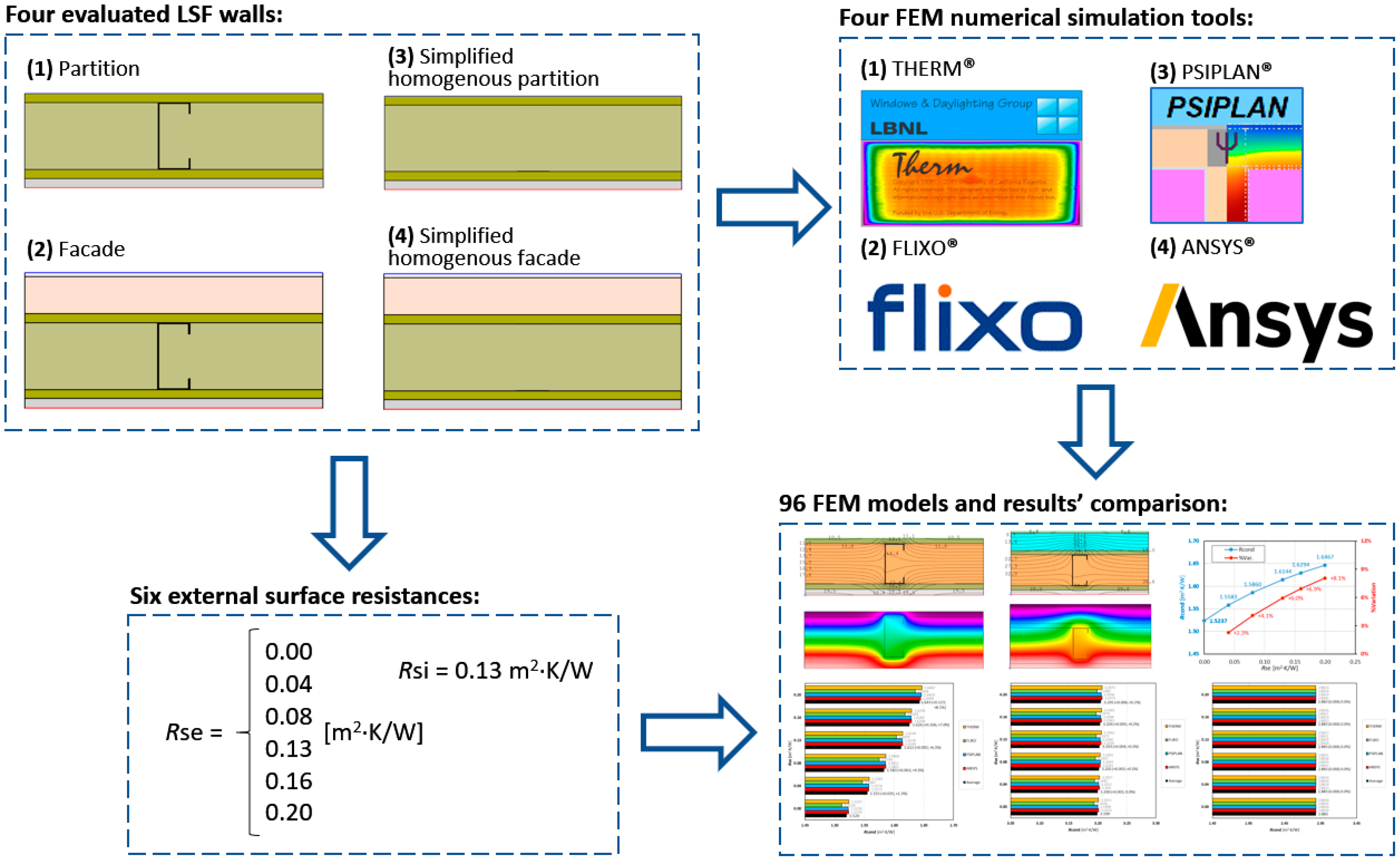
2.1. Walls Description and Material Characterization

In Figure 1 is presented the horizontal cross-sections of the partition and facade load-bearing LSF walls that are studied in this paper. The partition LSF wall is 126.5 mm thick and possesses vertical steel studs spaced 400 mm apart (with a web of 90 mm, a flange of 43 mm, a lip return of 15 mm and a thickness of 1.5 mm (C90 × 43 × 15 × 1.5)), Mineral Wool (MW) filling the entirety of the 90 mm air cavity, one oriented strand board (OSB) structural sheathing panel 12 mm thick on both sides of the steel studs, and a gypsum plasterboard (GPB) sheathing layer 12.5 mm thick on the inner surface. The facade LSF wall, besides having the same configuration as the partition wall, also has on the outer surface an internal thermal insulation composite system (ETICS), with expanded polystyrene (EPS) insulation 50 mm thick and a 5 mm layer of ETICS finishing, adding up to a 181.5 mm wall thickness. It should be noted that the LSF wall configurations evaluated in this study are existing ones, which are widely recognized in the field. They are usual LSF wall configurations for cold frame (Figure 1a) and hybrid (Figure 1b) construction systems [17], and have been already studied in previous research [20,21,22].
Besides these two LSF walls arrangements, another two simplified configurations were assessed to evaluate the relevance of the inhomogeneity of the material layer’s thermal conductivity. Thus, in these two additional wall configurations, the steel frames were removed to obtain a partition and a facade wall with homogeneous layers.
The thicknesses of each material layer and the corresponding thermal conductivities of these materials are listed in Table 1.

2.2. Adopted Methodology

After defining the four LSF walls’ configurations ((1) partition; (2) facade; (3) simplified homogenous partition, and (4) simplified homogenous façade), it was decided to model these walls by making use of four different FEM computational tools, as listed and explained later (please see Section 3.1), and as illustrated in Figure 2. Further details on the performed numerical simulations are provided in Section 3, including: (Section 3.2) domain discretization and boundary conditions, and (Section 3.3) accuracy verifications and validation.
The implemented models allowed us to compute the overall (or total) thermal resistance for each assessed wall, assuming six external surface resistances ( R s e ), ranging between 0.00 and 0.20 m2·K/W, and one internal surface resistance ( R s i ), i.e., 0.13 m2·K/W. The conductive thermal resistances ( R cond ), or surface-to-surface R -values, have been obtained by subtracting the considered R s e and R s i from the previously computed overall R -value. Next, the conductive thermal resistances for the 96 implemented models are analyzed, compared and discussed (Section 4). Finally, the main conclusions and remarks about this research work are presented in Section 5.

3. Numerical Simulations

3.1. Evaluated FEM Computational Tools

The numerical simulations of the evaluated LSF walls were performed using four different types of finite elements method (FEM) software: THERM (version 7.8) [29]; FLIXO (version 8.2) [30]; PSIPLAN (version 2024) [31], and ANSYS (student version 2022 R1) [32], where the first three are bi-dimensional (2D), and the last one allows for three-dimensional (3D) models. In the following subsections, some of the details of these software types and the respective numerical models are explained.
Starting with the THERM software [29], this is a state-of-the-art computer program, which is being developed in the Lawrence Berkeley National Laboratory, United States Department of Energy, and makes use of an FEM algorithm to analyse bi-dimensional heat-transfer effects in a steady-state regime. This computational tool creates an automatic mesh for the FEM analysis, which is based on two parameters. The first one is the threshold for the error of the iterative calculations (“Maximum % Error Energy Norm”), which, in this research, is set at 2%. The second one is the relative size of the finite element mesh of the model (“Quad Tree Mesh Parameter”), which was set to a standard value of 6. Regarding the definition of boundary conditions, besides the environmental temperatures, this software uses film coefficients (or surface heat transfer coefficients), which are the inverse of the surface thermal resistances.
FLIXO software [30] is a finite element analysis computational tool used for assessing 2D thermal bridges in a steady-state. This tool employs four main input features to create an automatic mesh for the implementation of the FEM model. The first is that the mesh can automatically consider the requirements prescribed in standard ISO 10211 [33]. Next, a minimum inside element angle of the triangular shape, set to 20 degrees, is required. After that, a maximum element size should be defined, which was set to 1:150 for this research. Lastly, both maximum values for the relative error and the heat flux error were defined as 1.0 × 10⁻³⁰ and 1.0 × 10⁻⁴, respectively.
Regarding the PSIPLAN 2D [31] software, this was designed to analyze two-dimensional heat transfer within a steady-state thermal regime, employing the plane heat transfer differential equation as its foundational computational model. The input of data is facilitated through a graphical module, offering an intuitive interface for users to define the spatial, geometrical, and thermo-technical characteristics of the subject under investigation. This includes specifying boundary conditions through superficial thermal resistances, interior and exterior temperatures, and relative humidity levels.
The program automates the meshing process for thermal bridge junctions by determining the meshing steps according to the specific requirements of the element under study and the simulation’s objectives, as outlined in Annex C, subsection C.2.c. of standard ISO 10211 [33]. This process involves formulating equilibrium equations at each node within the mesh, leading to the determination of temperature fields upon the resolution of the equation system.
Furthermore, the software adheres to stringent numerical validation criteria for meshing, as detailed in Annex C, subsection C.2. [33]. This section elucidates the methodology for deciding the number of subdivisions and establishes the necessary convergence criteria to ensure the accuracy and reliability of the simulation outcomes. The same discretization network was used for both the homogeneous element case and the inhomogeneous element case, using the same discretization steps and, implicitly, the same total number of discretization axes in the two directions.
To enhance the precision of the PSIPLAN simulations, specific attention was paid to the mesh size step, opting for a finer resolution starting from 0.2 mm. This choice is crucial to ensuring the accuracy of the results, and is particularly relevant to the domain discretization process described in Section 3.2. of ISO 10211 [33].
ANSYS Workbench [32] is a software that provides access to a suite of engineering simulation tools. It allows users to perform various simulations, such as structural, thermal, fluid dynamics, and electromagnetic simulations, among others. The ANSYS Workbench is widely used in engineering and product development to analyse and optimize designs before physical prototypes are built. In this research, the functionality of a steady-state thermal condition was used to simulate the thermal behaviour of construction elements. Among other features, this computational tool automatically creates and refines the mesh used for the FEM analysis. The main boundary conditions are the environmental temperature and the film coefficients. Regarding the mesh, in this study, an initial uniform mesh of 2 mm was used, and the borders between different materials were further automatically refined.

3.2. Domain Discretization and Boundary Conditions

As illustrated in Figure 1, only a 400 mm representative width segment of the LSF walls’ cross-section was modelled, so as to reduce computation time and effort. The dimensions and thermal conductivities of the materials used in the simulations are displayed in Table 1.
To perform the numerical simulations, the environmental air temperatures and surface thermal resistances have been defined. In this research, the interior air temperature was set to 20 °C, while the exterior one was set to 0 and 10 °C, for the facade and partition LSF walls, respectively. Therefore, the average temperature of the partition LSF walls is 15 °C, while for the facade LSF walls it is 10 °C. Table 2 displays the surface thermal resistances adopted. For the internal surface thermal resistance ( R s i ), we adopted the default value of 0.13 m2·K/W, recommended in standard ISO 6946 [9] for horizontal heat flow. To compare their influence over the computed thermal resistance, six distinct values, ranging from 0 to 0.20 m2·K/W, were simulated for the external surface thermal resistance ( R s e ). One of these was the ISO-recommended conventional R s e , i.e., 0.04 m2·K/W. The conventional surface thermal resistances suggested by ISO 6946 [9] range from 0.04 to 0.17 m2·K/W. Thus, we sought to cover this interval, starting at 0.00 (theoretical) and extending up to 0.20 m2·K/W.
To demonstrate that the mesh configuration and calculation approach employed are sufficiently robust for the simulation, a sensitivity analysis case study for the inhomogeneous partition wall using the PSIPLAN program is here presented. The boundary conditions were R s i = 0.13 m2·K/W and R s e = 0.04 m2·K/W, while the interior temperature was 20 °C and the exterior temperature was 10 °C. Therefore, the sensitivity analysis was conducted in two stages, as is presented below. The choice of the rectangular discretization network has been validated over the years through the program’s development, demonstrating that it provides quick convergence in the resolution of the system of energy balance equations.
  • First stage
The first step was to select a discretization mesh in accordance with criterion C2.d of standard ISO 10211 [33], which mandates that the number of subdivisions should be determined based on a process whereby the sum of the absolute values of all the thermal fluxes entering the object is assessed twice, once for n nodes (or cells) and then for 2 × n nodes (or cells). The variation between these two assessments must not surpass 1%. If it does, the number of subdivisions must be expanded until the requirement is fulfilled.
In the tabulated data presented (see Figure 3 and Table 3), various discretization node counts are employed to elucidate the impact of mesh refinement on the thermal flux, which serves as a critical parameter in the sensitivity analysis. Upon careful scrutiny of the thermal flux alterations consequent to the doubling of discretization nodes, it can be concluded that there is an inverse correlation between the increase in discretization nodes and the percentage deviation in heat flux ( ϕ s i ). This trend is indicative of the system’s convergence characteristics.
As can be observed, the condition is met starting from node count of 1739 onwards. Beyond this threshold, any augmentation in node count, characterized by doubling, yields a variance in the calculated thermal flux that is within the permissible limit of less than 1%, thereby affirming the adequacy of the mesh configuration for the thermal simulations conducted. The final row in Table 3 lists the R -values for all evaluated cases, capturing the impact of thermal bridges on the detailed thermal performance.
  • Second stage
Based on the results presented in Table 3, the second step of the analysis involved confirming the computational precision of temperature and flux values to meet the criterion specified in condition C2.e of standard ISO 10211 [33]. This condition necessitates that for iterative solution methods, iterations should proceed until the ratio of the sum of all thermal fluxes (positive and negative) entering the object to the semi-sum of their absolute values is below 0.0001.
Taking into account the stipulation in section C.2.b of standard ISO 10211 [33], which states that the subdivision degree of the object (specifically, the number of cells or nodes) is at the discretion of the user rather than being predetermined by the computational method, and referring to the outcomes highlighted in stage 1, a subdivision size of 0.5 mm was consistently utilized throughout this case study.
Observing the precision row in the results (see Table 4), it can be seen that the precision of the iterative calculations consistently improves, eventually achieving and surpassing the required threshold of less than 0.0001. This is evidenced by the final entries in the precision row, which meet the rigorous precision requirement laid out in condition C2.e of standard ISO 10211 [33].

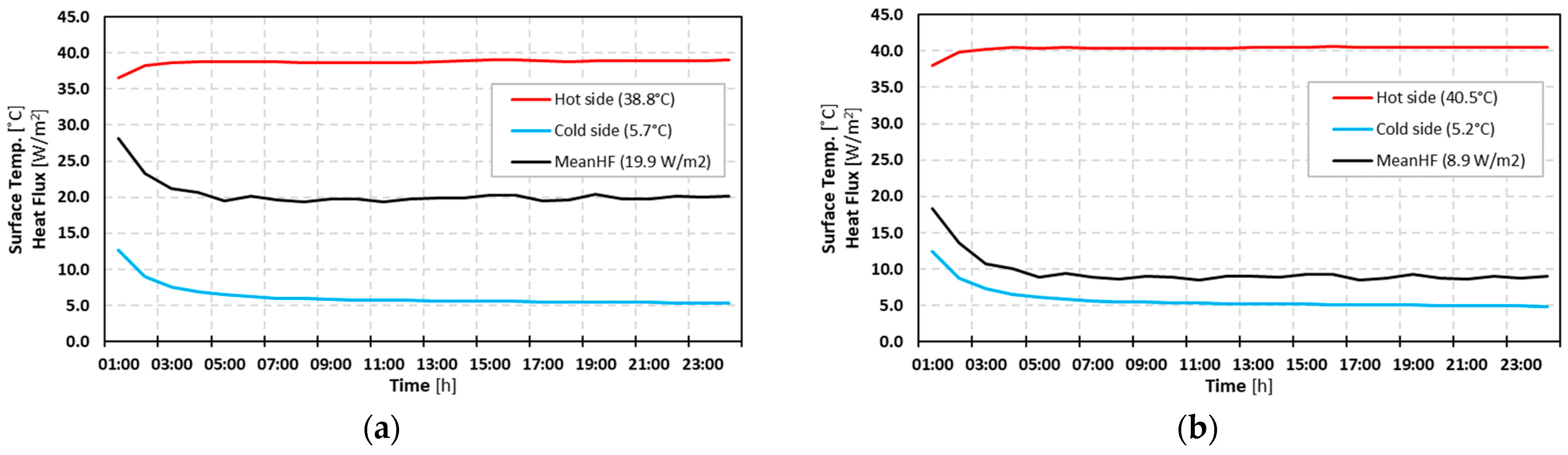
3.3. Model Accuracy Verifications and Validation

The authors already have a large degree of experience in using three of these computational tools, as can be verified in the following published papers, regarding THERM [18,20,21,22,23,34,35,36,37,38,39,40], ANSYS [21,22,34,38,39,41,42] and PSIPLAN [12,43,44,45,46,47,48,49]. Only the FLIXO software is being used by the authors for the first time, but with excellent results, as can be checked afterwards.
Nevertheless, several accuracy verifications and one validation by comparison to measurements were performed. The accuracy verifications that were performed were based on the test cases defined in Annex C of standard ISO 10211 [33], as well as in the analytical calculation procedures defined in standard ISO 6946 [9], for homogeneous layers. Moreover, the implemented models were validated by comparing some results with laboratory measurements under controlled conditions. These verification and validation procedures will be briefly described in the following paragraphs.
To ensure the precision of the computational tools used and the models implemented, the first two bi-dimensional test cases prescribed in Annex C of ISO 10211 [33] were simulated, and the following 3D test cases (3 and 4) from the same standard [33] were modelled in ANSYS (the only three-dimensional tested algorithm). The obtained results were within the permitted bounds, the difference between temperatures calculated and listed not exceeding 0.1 °C and the difference between heat flow values not exceeding 0.1 W/m.
The second verification was a comparison of the obtained thermal transmittances for the models previously presented in Figure 1, but simplified (i.e., without steel studs), with the results provided by the analytical calculation procedures provided in standard ISO 6946 [9] for walls with homogeneous layers. The material properties were the ones previously specified in Table 1, and the boundary conditions have also previously been described (please see Section 3.2), the values of the implemented surface thermal resistances being equal to the conventional ones defined in ISO 6946 [9], i.e., 0.13 and 0.04 m2·K/W for R s i and R s e , respectively. Notice that for the partition, we adopted R s e , equal to R s i (0.13 m2·K/W), since both walls’ sides are internal (it is a load-bearing partition, instead of a facade).
Table 5 displays the overall thermal transmittances obtained for the analytical and numerical approaches, for both types of evaluated walls (simplified partition and facade). As expected, for each wall type, the U values are equal until the third decimal place, ensuring the excellent accuracy of the evaluated algorithms and models.
The third strategy to ensure the accuracy of the evaluated LSF wall models was an experimental validation based on laboratory measurements. Making use of two load-bearing LSF wall prototypes ((1) a partition [20] and (2) a facade, as illustrated in Figure 4), their surface-to-surface thermal resistances were measured under controlled lab conditions. The LSF wall prototypes were placed between a hot box (heated by a thermal resistance up to around 40 °C) and a cold box (cooled by a fridge down to around 5 °C). These kinds of “climatic chambers” allowed us to implement a nearly steady-state temperature difference between the tested LSF walls of around 35 °C, for a mean average temperature of the tested LSF walls equal to 22.5 °C. To mitigate the eventual flanking lateral heat losses, the perimeter for the tested LSF wall was covered with polyurethane foam insulation (80 mm thick), while it was supported by a layer of more rigid thermal insulation (100 mm thick XPS).
The heat transfer across the tested LSF wall samples was monitored by making use of thermocouples (TC) to measure temperatures, and Heat Flow Meters (HFMs) to measure heat flux. These measurements were performed making use of the Heat Flow Meter method described in standard ISO 9869-1 [7]. However, to improve the measurements’ accuracy and reduce the test duration, two HFMs were used simultaneously, for each sensor location, at both cold and hot wall surfaces, as suggested by Rasooli and Itard [50].
For each wall configuration, three tests were performed; for each test, the sensors were placed at different height locations, as illustrated in Figure 4b. Moreover, these measurements were performed along two vertical lines: (1) in the middle of the LSF wall prototype, i.e., near the vertical steel stud, and (2) between the steel studs, i.e., in the middle of the insulation cavity. This test setup allowed us to monitor the two typical thermal behaviour zones on an LSF wall: (1) a region with higher heat flux (HFM1), originated by the steel stud’s thermal bridge, and (2) the remaining part of the wall with smaller heat flux (HFM2), due to the cavity thermal insulation. More details about these measurements could be found in previous research works published by the authors [20,35].
Besides the measured conductive thermal resistances, displayed in Table 6 as R cond , it was possible to also measure the average surface thermal resistances for each side of the tested LSF walls. The measured values were, for the partition LSF wall, R s i = 0.10 m2·K/W and R s e = 0.11 m2·K/W, and for the facade, R s i = 0.10 m2·K/W and R s e = 0.13 m2·K/W. Notice that the internal surface resistance ( R s i ) was measured on the hot side of the tested wall, while the external one ( R s e ) was measured on the cold side of the same wall.
Figure 5 displays the measured heat flux values and surface temperatures over time (24 h) for the facade LSF wall, when the sensors were located at the highest height, as illustrated in Figure 4b. The measured values recorded at two different sensor locations are displayed in these plots: (1) near the steel stud (Figure 5a), and (2) in the wall cavity (Figure 5b). It is clearly visible that after a couple of hours, the values stabilize, confirming the intended steady-state regime. Regarding surface temperatures, the values are quite similar at both sensor locations (around 40 °C and 5 °C). As expected, the major difference is related to the heat flux values, these being much bigger (around 19.9 W/m2) near the steel stud (Figure 5a) when compared to the cavity location (near 8.9 °C), due to the thermal bridge effect caused by the high thermal conductivity of steel.
Making use of the measured values (surface thermal resistances and environmental air temperatures on both sides of the wall), it was possible to model a similar representative partition and facade LSF wall, making use of the four tested FEM computational tools. Afterwards, we computed the predicted conductive (or surface-to-surface) thermal resistance ( R c o n d ) for each wall and each software model, as displayed in Table 6.
When comparing the results predicted by the FEM models with the measurements, we can see very good agreement, whereby the differences vary between −0.1% and +2.3%. Moreover, these deviations are much smaller (almost negligible) for the facade LSF wall, this being explained by the steel studs’ lower thermal bridge relevance, given the effect of the continuous external thermal insulation layer (ETICS). These results allow us to validate the accuracy of the implemented models, making use of the four computational tools compared in this research.

4. Results and Discussion

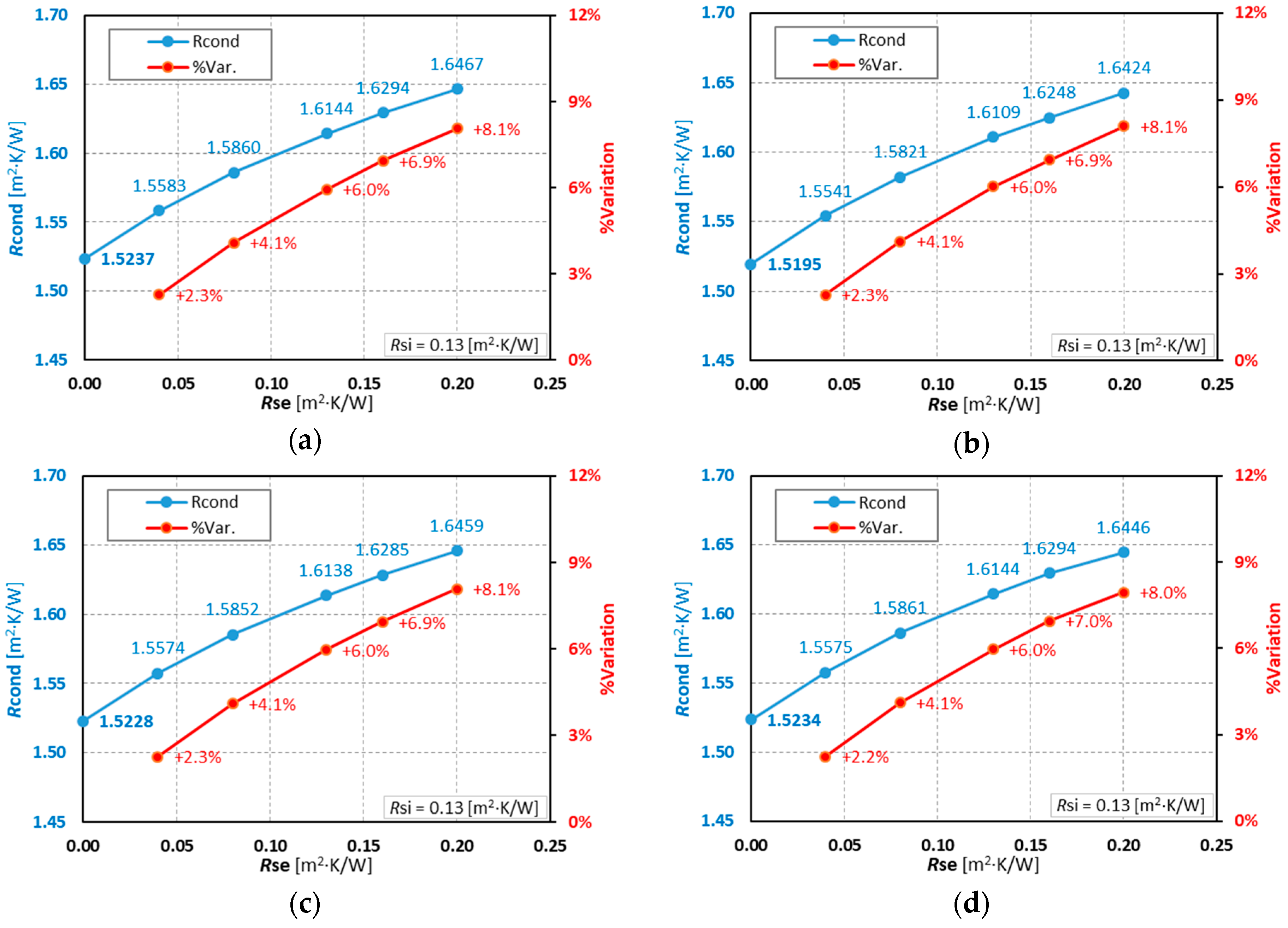
4.1. Partition LSF Walls

Regarding the partition LSF walls, Figure 6 displays the surface-to-surface or conductive thermal resistances ( R c o n d ) computed for several external surface thermal resistances ( R s e ) within the range of 0.0–0.20 m2·K/W, making use of the four evaluated FEM computational tools.
As expected, the lowest R c o n d value is provided for the smaller R s e , i.e., assuming a null value. Regarding the THERM software (Figure 6a), the computed surface-to-surface thermal resistance is 1.5237 m2·K/W. When the R s e value is increased up to 0.20 m2·K/W, there is also a non-linear increase in the R c o n d value (greater increment for smaller R s e values), reaching a maximum value of 1.6467 m2·K/W, which corresponds to an increase of +0.123 m2·K/W (+8.1%). Notice that for the other evaluated computational tools, i.e., FLIXO (Figure 6b), PSIPLAN (Figure 6c) and ANSYS (Figure 6d), the trend is very similar, as are the computed values.
To better visualize and compare the results for the several tested FEM computational tools, Figure 7 displays all the obtained R c o n d values in a single plot, as well as the averaged computed values for each external surface thermal resistance value. This graph makes it clearer that the thermal resistances computed by THERM, PSIPLAN and ANSYS are very similar, while the ones provided by the FLIXO algorithm are slightly smaller.
Looking now at the averaged R c o n d values, the trend is very similar to the one previously observed in Figure 6, i.e., there is a non-linear increase ranging from the minimum (1.520 m2·K/W) up to a maximum conductive thermal resistance of 1.643 m2·K/W, corresponding to an increase of +0.123 m2·K/W (+8.1%). Notice that these average thermal resistance increments (absolute and percentage) are the same as those previously observed and discussed in relation to the THERM software (Figure 6a).

4.2. Facade LSF Walls

In this section, the results obtained for the facade LSF walls are presented and discussed. Notice that the main difference between the previously evaluated LSF partition (Section 4.1) and this LSF facade is that the latter has an additional ETICS layer containing 50 mm of EPS insulation, as previously illustrated in Figure 1b and listed in Table 1. This fact results in an LSF facade wall wherein the thermal bridges due to the steel studs are less relevant, given the existence of a continuous ETICS insulation layer.
Figure 8 illustrates the conductive thermal resistance values ( R c o n d ) computed for the evaluated LSF facade wall. Comparing these results with the previous ones derived for the partition LSF wall (Figure 7), the main difference, besides the higher thermal resistances obtained (around two times higher), is that now the increase in R c o n d values for higher external surface values is greatly reduced. In fact, this average increment is only from 3.199 up to 3.205 m2·K/W, corresponding to an absolute increase of +0.006 m2·K/W (+0.2%). This feature leads us to conclude that the relevance of the surface thermal resistance values to the conductive thermal resistance in LSF facade walls, with the thermal bridges of steel studs being adequately mitigated (e.g., by an ETICS layer), is notably reduced, and is almost negligible.

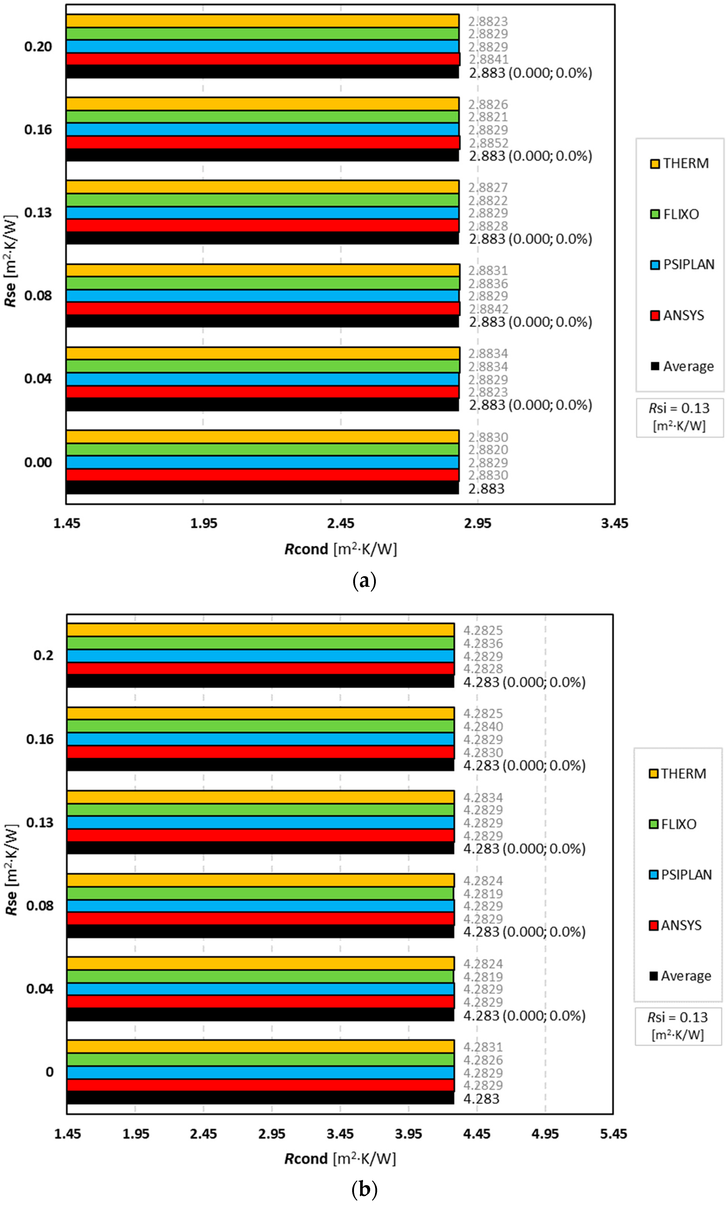
4.3. Homogeneous Layered Walls

To confirm the previous assumption that the relevance of surface thermal resistance variations to the corresponding R c o n d values significantly decreases when the thermal bridge effect in the wall also decreases or becomes non-existent (unidirectional heat transfer), we here discuss the results computed for both partition and facade homogeneous layered walls, i.e., without steel studs (no thermal bridges).
Figure 9 displays the surface-to-surface thermal resistances computed for the partition (Figure 9a) and facade (Figure 9b) LSF walls, but here assuming homogeneous layered walls, i.e., neglecting the steel frame. The values for each wall type are nearly constant, and do not depend on the surface thermal resistances. On average, the computed conductive thermal resistances are equal to 2.883 and 4.283 m2·K/W for the partition and facade walls, respectively.
These results also allow us to perform an additional verification of the implemented models and algorithms, since the provided results could be compared and should be equal to the ones provided by analytical calculations performed for homogenous layers (ISO 6046 [9]). Making use of the thicknesses and thermal conductivities previously provided in Table 1, the thermal resistance provided by each wall layer could be obtained. Summing all these thermal resistances, we obtain the same conductive R -values as those displayed in Figure 9a,b, ensuring again the accuracy of the implemented numerical models using the four evaluated computational tools.

4.4. Results Overview

To allow for the better and easier analysis of the results, Figure 10 shows only the averaged R c o n d values computed using the four FEM computational tools, as well as their percentage variations. Regarding the partition LSF wall (Figure 10a), we can now even more clearly see the increase in the conductive thermal resistance values, from 1.522 up to 1.645 m2·K/W, corresponding to a percentage variation up to +8.1%.
Observing now the results obtained for the facade LSF wall (Figure 10b), we can see that the R c o n d averaged values are nearly constant, showing only a slight increase from 3.199 up to 3.205 m2·K/W, which also means a minimal percentage variation up to +0.2%.
The R c o n d values for homogeneous simplified LSF walls (i.e., without the steel frame) are constant, and do not change with the increment of the external surface thermal resistances, as previously seen before in Section 4.3.
To better understand and visualize the obtained results, Figure 11 displays the average computed conductive thermal resistances ( R c o n d ) and the corresponding temperature color distribution predicted by the THERM models for the two extreme surface thermal resistances ( R s e ), these being 0.0 m2·K/W for the first column and 0.20 m2·K/W for the second (right one). Three different wall configurations were selected for this analysis, namely: (a) partition LSF wall; (b) facade LSF wall, and (c) facade, homogenous simplified wall.
Looking to the partition LSF wall cross-section temperature distributions (Figure 11a), and comparing the results for both surface thermal resistances, it is clearly visible that, near the external wall surface, there are some differences, the major ones being near the flange of the steel stud, as a result of the related thermal bridge effect. In fact, for the higher R s e (0.20 m2·K/W) the external surface temperatures are also higher, as expected, in comparison to the other R s e value.
We can also observe similar results for the facade LSF wall cross-sections (Figure 11b); given the external continuous insulation layer (ETICS), the steel stud’s thermal bridge effect is now more attenuated, mainly near the external wall surface, where the temperature values are almost constant for both R s e values. These features elucidate the reason why, in this LSF wall configuration, the conductive thermal resistances are almost the same, with an increment of only +0.2%.
Regarding the simplified facade wall with homogenous layers, i.e., without steel studs (Figure 11c), as expected, the computed colour distribution is steady over all the layers of the wall, corresponding to a perfect unidirectional heat transfer without any thermal bridge effect. Therefore, the R c o n d values are now fixed for all evaluated surface thermal resistances. Obviously, besides being fixed, the surface-to-surface R -value is now bigger (4.283 m2·K/W) when compared with the previous LSF wall configuration (3.200 m2·K/W), corresponding to an increment of 1.083 m2·K/W (+33.8%).

5. Conclusions

In this work, the influence of surface thermal resistance ( R s ) on the conductive thermal resistance ( R c o n d ) of LSF walls was evaluated. To this end, four finite elements’ numerical simulation tools were used to model the four assessed LSF walls, showing different levels of thermal conductivity inhomogeneity: (1) partition, cold frame LSF wall; (2) facade, hybrid LSF wall; (3) simplified homogeneous partition LSF wall, and (4) simplified homogeneous facade LSF wall. Moreover, six external thermal surface resistances ( R s e ) were modeled, ranging from 0.00 up to 0.20 m2·K/W. The average temperature of the partition LSF walls is 15 °C, while for the facade LSF walls it is 10 °C.
Notice that the accuracy of the implemented numerical models used in this study was verified, taking as a reference the ISO 10211 test cases and the ISO 6946 analytical calculation rules for homogeneous layered simplified walls, as well as by comparing the results provided by the four evaluated computational tools. Moreover, the precision of the employed models was also validated by comparison to measurements under controlled lab conditions.
The main conclusions of this research work can be listed as follows:
  • The accuracy of all evaluated computational tools was very high and similar;
  • The R c o n d value is nearly uniform for walls with homogeneous layers, as expected;
  • The variation of the R c o n d values depends on the level of inhomogeneity in the LSF wall layers;
  • For the assessed R s e values, the conductive thermal resistances increased up to 8.1%, i.e., +0.123 m2·K/W, for the partition cold frame LSF wall;
  • However, the variation in R c o n d values was almost negligible (only up to +0.2%) for the facade hybrid LSF wall with a continuous thermal insulation layer (50 mm thick);
  • When removing the steel frames, the R c o n d values of this simplified facade wall do not change, regardless of the R s e values;
  • However, when compared to the original LSF facade wall, the conductive thermal resistance values increased significantly (+34%);
  • Numerical modelling and laboratory measurements are complementary methods, and the combination of them boosts the accuracy and the practical relevance of thermal performance analyses.

Author Contributions

Conceptualization, P.S. and L.M.; methodology, P.S. and L.M.; software, P.S., D.A., P.L. and L.M.; validation, P.S., D.A., P.L. and L.M.; formal analysis, P.S. and L.M.; investigation, P.S.; resources, P.S.; writing—original draft preparation, P.S. and L.M.; writing—review and editing, P.S. and L.M.; visualization, P.S.; supervision, P.S.; project administration, P.S. and L.M.; funding acquisition, P.S. and L.M. All authors have read and agreed to the published version of the manuscript.

Funding

This work was funded using FEDER funds from the Competitivity Factors Operational Programme—COMPETE and national funds form FCT—Foundation for Science and Technology within the scope of the project POCI-01-0145-FEDER-032061. This work was also supported by a grant of the Ministry of Research, Innovation and Digitization, CCCDI—UEFISCDI, project number PN-III-P2-2.1-PED-2021-4137, within PNCDI III—CT 714PED/2022.

Institutional Review Board Statement

Not applicable.

Informed Consent Statement

Not applicable.

Data Availability Statement

The data presented in this study are available in article.

Conflicts of Interest

The authors declare no conflicts of interest.

References

  1. European Parliament Directive 2002/91/EC of the European Parliament and of the Council of 16 December 2002 on the Energy performance of Buildings. Off. J. Eur. Commun. 2002, L1/65–L1/71.
  2. European Parliament. Energy Performance of Buildings (Recast), European Parliament Legislative Resolution of 12 March 2024 on the Proposal for a Directive of the European Parliament and of the Council on the Energy Performance of Buildings (Recast), COM(2021)0802–C9-0469/2021–2021/0426(COD); European Parliament: Strasbourg, France, 2024.
  3. Wang, H.; Zhai, Z. (John) Advances in Building Simulation and Computational Techniques: A Review between 1987 and 2014. Energy Build. 2016, 128, 319–335. [Google Scholar] [CrossRef]
  4. Vera-Piazzini, O.; Scarpa, M. Building Energy Model Calibration: A Review of the State of the Art in Approaches, Methods, and Tools. J. Build. Eng. 2024, 86, 108287. [Google Scholar] [CrossRef]
  5. Crawley, D.B.; Hand, J.W.; Kummert, M.; Griffith, B.T. Contrasting the Capabilities of Building Energy Performance Simulation Programs. Build. Environ. 2008, 43, 661–673. [Google Scholar] [CrossRef]
  6. Kim, S.-H.; Kim, J.-H.; Jeong, H.-G.; Song, K.-D. Reliability Field Test of the Air–Surface Temperature Ratio Method for In Situ Measurement of U-Values. Energies 2018, 11, 803. [Google Scholar] [CrossRef]
  7. ISO 9869-1; Thermal Insulation—Building Elements—In-Situ Measurement of Thermal Resistance and Thermal Transmittance. Part 1: Heat Flow Meter Method. ISO: Geneva, Switzerland, 2014.
  8. Evangelisti, L.; Guattari, C.; Asdrubali, F. Comparison between Heat-Flow Meter and Air-Surface Temperature Ratio Techniques for Assembled Panels Thermal Characterization. Energy Build. 2019, 203, 109441. [Google Scholar] [CrossRef]
  9. ISO 6946; Building Components and Building Elements—Thermal Resistance and Thermal Transmittance—Calculation Methods. ISO: Geneva, Switzerland, 2017.
  10. De Rubeis, T.; Evangelisti, L.; Guattari, C.; De Berardinis, P.; Asdrubali, F.; Ambrosini, D. On the Influence of Environmental Boundary Conditions on Surface Thermal Resistance of Walls: Experimental Evaluation through a Guarded Hot Box. Case Stud. Therm. Eng. 2022, 34, 101915. [Google Scholar] [CrossRef]
  11. Arregi, B.; Garay-Martinez, R.; Astudillo, J.; García, M.; Ramos, J.C. Experimental and Numerical Thermal Performance Assessment of a Multi-Layer Building Envelope Component Made of Biocomposite Materials. Energy Build. 2020, 214, 109846. [Google Scholar] [CrossRef]
  12. Moga, L.; Moga, I. Thermal Bridges at Wood Frame Construction. J. Appl. Eng. Sci. 2015, 5, 65–71. [Google Scholar] [CrossRef]
  13. Murtinho, V.; Ferreira, H.; Antonio, C.; Simoes da Silva, L.; Gervasio, H.; Santos, P. Architectural Concept for Multi-Storey Apartment Building with Light Steel Framing. Steel Constr. 2010, 3, 163–168. [Google Scholar] [CrossRef]
  14. Santos, P.; Mateus, D.; Simoes Da Silva, L.; Rebelo, C.; Gervasio, H.; Correia, A.; Ferreira, H.; Santiago, A.; Murtinho, V.; Rigueiro, C. Affordable Houses (Part II): Functional, Structural and Technological Performance. In Proceedings of the Structures and Architecture—Proceedings of the 1st International Conference on Structures and Architecture, ICSA 2010, Guimaraes, Portugal, 21–23 July 2010. [Google Scholar]
  15. Soares, N.; Santos, P.; Gervásio, H.; Costa, J.J.; Simões da Silva, L. Energy Efficiency and Thermal Performance of Lightweight Steel-Framed (LSF) Construction: A Review. Renew. Sustain. Energy Rev. 2017, 78, 194–209. [Google Scholar] [CrossRef]
  16. de Angelis, E.; Serra, E. Light Steel-Frame Walls: Thermal Insulation Performances and Thermal Bridges. Energy Procedia 2014, 45, 362–371. [Google Scholar] [CrossRef]
  17. Santos, P.; da Silva, L.S.; Ungureanu, V. Energy Efficiency of Light-Weight Steel-Framed Buildings, 1st ed.; Technical Committee 14—Sustainability & Eco-Efficiency of Steel Construction; European Convention for Constructional Steelwork (ECCS): Mem Martins, Portugal, 2012; ISBN 978-92-9147-105-8. [Google Scholar]
  18. Santos, P.; Lemes, G.; Mateus, D. Analytical Methods to Estimate the Thermal Transmittance of LSF Walls: Calculation Procedures Review and Accuracy Comparison. Energies 2020, 13, 840. [Google Scholar] [CrossRef]
  19. Santos, C.; Matias, L. ITE50—Coeficientes de Transmissão Térmica de Elementos Da Envolvente Dos Edifícios; LNEC—Laboratório Nacional de Engenharia Civil: Lisboa, Portugal, 2006. (In Portuguese) [Google Scholar]
  20. Santos, P.; Mateus, D. Experimental Assessment of Thermal Break Strips Performance in Load-Bearing and Non-Load-Bearing LSF Walls. J. Build. Eng. 2020, 32, 101693. [Google Scholar] [CrossRef]
  21. Santos, P.; Lopes, P.; Abrantes, D. Thermal Performance of Lightweight Steel Framed Facade Walls Using Thermal Break Strips and ETICS: A Parametric Study. Energies 2023, 16, 1699. [Google Scholar] [CrossRef]
  22. Santos, P.; Poologanathan, K. The Importance of Stud Flanges Size and Shape on the Thermal Performance of Lightweight Steel Framed Walls. Sustainability 2021, 13, 3970. [Google Scholar] [CrossRef]
  23. Roque, E.; Santos, P. The Effectiveness of Thermal Insulation in Lightweight Steel-Framed Walls with Respect to Its Position. Buildings 2017, 7, 13. [Google Scholar] [CrossRef]
  24. Gyptec Ibérica Technical Sheet: Standard Gypsum Plasterboard. Available online: https://gyptec.eu/en/ (accessed on 10 February 2022).
  25. Kronospan Technical Sheet: Kronobuild Materials. Available online: https://de.kronospan-express.com/public/files/downloads/kronobuild/kronobuild-en.pdf (accessed on 10 February 2022).
  26. Volcalis Technical Sheet: Alpha Mineral Wool. Available online: https://volcalis.pt/ (accessed on 10 February 2022).
  27. LNEC Documento de Homologação: Tincoterm EPS—Sistema Compósito de Isolamento Térmico Pelo Exterior. Available online: http://www.lnec.pt/fotos/editor2/tincoterm-eps-sistema-co-1.pdf (accessed on 10 February 2022). (In Portuguese).
  28. WEBERTHERM UNO Technical Sheet: Weber Saint-Gobain ETICS Finish Mortar. Available online: https://construir.saint-gobain.pt/ (accessed on 10 February 2022). (In Portuguese).
  29. THERM Software Version: 7.8.57.0. Available online: https://windows.lbl.gov/therm-software-downloads (accessed on 14 February 2023).
  30. FLIXO Software Trial Version: 8.2.1178.1. Available online: https://www.flixo.com (accessed on 25 March 2024).
  31. Moga, I.; Moga, L. Model. Simul. Two-Dimensional Heat Transf. Build, PSIPLAN Software Version 2024. 2024.
  32. ANSYS Workbench: Steady-State Thermal Software Version: Student 2022 R1. Available online: https://www.ansys.com/academic/students/ansys-student (accessed on 10 February 2022).
  33. ISO 10211; Thermal Bridges in Building Construction—Heat Flows and Surface Temperatures—Detailed Calculations. International Organization for Standardization: Geneva, Switzerland, 2017.
  34. Santos, P.; Lopes, P.; Abrantes, D. Thermal Performance of Load-Bearing, Lightweight, Steel-Framed Partition Walls Using Thermal Break Strips: A Parametric Study. Energies 2022, 15, 9271. [Google Scholar] [CrossRef]
  35. Santos, P.; Mateus, D.; Ferrandez, D.; Verdu, A. Numerical Simulation and Experimental Validation of Thermal Break Strips’ Improvement in Facade LSF Walls. Energies 2022, 15, 8169. [Google Scholar] [CrossRef]
  36. Santos, P.; Ribeiro, T. Thermal Performance Improvement of Double-Pane Lightweight Steel Framed Walls Using Thermal Break Strips and Reflective Foils. Energies 2021, 14, 6927. [Google Scholar] [CrossRef]
  37. Santos, P.; Ribeiro, T. Thermal Performance of Double-Pane Lightweight Steel Framed Walls with and without a Reflective Foil. Buildings 2021, 11, 301. [Google Scholar] [CrossRef]
  38. Santos, P.; Gonçalves, M.; Martins, C.; Soares, N.; Costa, J.J. Thermal Transmittance of Lightweight Steel Framed Walls: Experimental Versus Numerical and Analytical Approaches. J. Build. Eng. 2019, 25, 100776. [Google Scholar] [CrossRef]
  39. Santos, P.; Martins, C.; Simoes da Silva, L.; Bragança, L. Thermal Performance of Lightweight Steel Framed Wall: The Importance of Flanking Thermal Losses. J. Build. Phys. 2014, 38, 81–98. [Google Scholar] [CrossRef]
  40. Santos, P.; Lemes, G.; Mateus, D. Mateus Thermal Transmittance of Internal Partition and External Facade LSF Walls: A Parametric Study. Energies 2019, 12, 2671. [Google Scholar] [CrossRef]
  41. Martins, C.; Santos, P.; Simoes da Silva, L. Lightweight Steel-Framed Thermal Bridges Mitigation Strategies: A Parametric Study. J. Build. Phys. 2016, 39, 342–372. [Google Scholar] [CrossRef]
  42. Santos, P.; Martins, C.; Júlio, E. Enhancement of the Thermal Performance of Perforated Clay Brick Walls through the Addition of Industrial Nano-Crystalline Aluminium Sludge. Constr. Build. Mater. 2015, 101, 227–238. [Google Scholar] [CrossRef]
  43. Moga, L.; Petran, I.; Santos, P.; Ungureanu, V. Thermo-Energy Performance of Lightweight Steel Framed Constructions: A Case Study. Buildings 2022, 12, 321. [Google Scholar] [CrossRef]
  44. Moga, L.; Moga, I. Specific Thermal Bridges at Load Bearing Masonry Buildings; UTPRESS: Cluj-Napoca, Romania, 2013. [Google Scholar]
  45. Moga, L.; Moga, I. Specific Thermal Bridges for Terrace Roofs, Attic Floors, Floors over the Basement and Slabs on the Ground at Load Bearing Masonry Buildings; UTPRESS: Cluj-Napoca, Romania, 2017. [Google Scholar]
  46. Marincu, C.; Dan, D.; Moga, L. Investigating the Influence of Building Shape and Insulation Thickness on Energy Efficiency of Buildings. Energy Sustain. Dev. 2024, 79, 101384. [Google Scholar] [CrossRef]
  47. Moga, L.; Moga, I. Numerical Modelling of Point Thermal Bridge’s Impact on the Thermal Performance of Facade Systems. IOP Conf. Ser. Mater. Sci. Eng. 2021, 1141, 012018. [Google Scholar] [CrossRef]
  48. Moga, L.; Moga, I. Evaluation of Thermal Bridges Using Online Simulation Software. E3S Web Conf. 2020, 172, 08010. [Google Scholar] [CrossRef]
  49. Moga, L.; Moga, I. Considerations on the Thermal Modelling of Insulated Metal Panel Systems. In Proceedings of the Healthy, Intelligent and Resilient Buildings and Urban Environments; International Association of Building Physics (IABP): Syracuse, New York, NY, USA, 23–26 September 2018; pp. 1235–1240. [Google Scholar]
  50. Rasooli, A.; Itard, L. In-Situ Characterization of Walls’ Thermal Resistance: An Extension to the ISO 9869 Standard Method. Energy Build. 2018, 179, 374–383. [Google Scholar] [CrossRef]
Figure 1. Evaluated load-bearing LSF walls’ horizontal cross-sections: (a) Partition; (b) facade LSF wall.
Applsci 14 03748 g001
Figure 2. Implemented methodology scheme.
Applsci 14 03748 g002
Figure 3. Mesh refinement stages in thermal simulation with visualization of temperature field for the LSF partition wall: (a) 16.0 mm; (b) 8.0 mm; (c) 4.0 mm; (d) 2.0 mm; (e) 1.0 mm; (f) 0.5 mm; (g) 0.2 mm; (h) temperature field at 0.2 mm.
Applsci 14 03748 g003
Figure 4. Tested load-bearing LSF facade prototype: (a) steel frame; (b) sensors’ position (cold surface) [35].
Applsci 14 03748 g004
Figure 5. Measured heat flux values and surface temperatures over time when sensors are located at the highest height (see Figure 4b) for the LSF facade: (a) Sensor position 1, near the steel stud. (b) Sensor position 2, in the middle of the wall cavity.
Applsci 14 03748 g005
Figure 6. Partition LSF wall: conductive thermal resistances ( R c o n d ) for different external surface thermal resistances ( R se ) and their percentage variation, computed using (a) THERM, (b) FLIXO, (c) PSIPLAN, and (d) ANSYS.
Applsci 14 03748 g006
Figure 7. Partition LSF wall: conductive thermal resistances ( R c o n d ) for different external surface thermal resistances ( R s e ) computed by different FEM softwares and their average value variations.
Applsci 14 03748 g007
Figure 8. Facade LSF wall: conductive thermal resistances ( R c o n d ) for different external surface thermal resistances ( R s e ) computed by different FEM softwares and their average value variations.
Applsci 14 03748 g008
Figure 9. Conductive thermal resistances ( R c o n d ) for different external surface thermal resistances ( R s e ) computed by different FEM softwares and their average value variations: (a) homogeneous partition; (b) homogeneous facade.
Applsci 14 03748 g009
Figure 10. Average values of computed conductive thermal resistances ( R c o n d ) for different external surface thermal resistances ( R s e ) and their percentage variation: (a) partition LSF wall, (b) facade LSF wall.
Applsci 14 03748 g010
Figure 11. Average computed conductive thermal resistances, with temperature showing colour distribution predicted by THERM models for the two extreme surface thermal resistances ( R s e ) and for different wall configurations: (a) partition LSF wall; (b) facade LSF wall; (c) simplified facade wall with homogenous layers (without steel studs).
Applsci 14 03748 g011
Table 1. Thickness, t , and thermal conductivity, λ, of materials [21].
Material t
(mm)
λ
(W/(m·K))
Ref.
Gypsum Plaster Board (GPB)12.50.175[24]
Oriented Strand Board (OSB)12.00.100[25]
Mineral Wool (MW)90.00.035[26]
Steel Studs (C90 × 43 × 15 × 1.5)90.050.000[19]
ETICS 2 Insulation (EPS 1)50.00.036[27]
ETICS 2 Finish5.00.450[28]
1 EPS—expanded polystyrene; 2 ETICS—external thermal insulation composite system.
Table 2. Evaluated internal ( R s i ) and external ( R s e ) surface thermal resistances.
R s i (m2·K/W)0.13
R s e (m2·K/W)0.000.040.080.130.160.20
Table 3. Analysis of convergence of thermal flux sensitivity to discretization node variation, regarding the LSF partition PSIPLAN model, for R s i and R s e values equal to 0.13 and 0.04 m2·K/W, respectively.
N. of nodes23450091017393795754619,468
Step size (mm)16.0 8.0 4.0 2.0 1.0 0.5 0.2
ϕ s i (W/model length)2.4363652.3732342.3465572.3319522.3229832.3184952.315669
Differences---−2.7%−1.1%−0.6%−0.4%−0.2%−0.1%
R c o n d (m2·K/W)1.4717901.5154641.5346251.5453011.5519241.5552571.557363
R -value (m2·K/W)1.6417901.6854641.7046251.7153011.7219241.7252571.727363
Table 4. Evaluation of iterative calculation precision in thermal flux analysis at 0.5 mm subdivision (7546 nodes), regarding the LSF partition PSIPLAN model, for R s i and R s e values equal to 0.13 and 0.04 m2·K/W, respectively.
Iterations1st 2nd 3rd 4th 5th 6th 7th
ϕ s i (W/model length)2.3595322.3225982.3189052.3185362.3184992.3184952.318495
ϕ s e (W/model length)2.2597202.3126172.3179072.3184362.3184892.3184942.318495
Precision0.0432150.0043070.0004310.0000430.0000040.0000000.000000
R c o n d (m2·K/W)1.5269441.5523811.5549691.5552281.5552541.5552571.555257
R -value (m2·K/W)1.6952521.7222091.7249521.7252271.7252541.7252571.725257
Table 5. Thermal transmittance calculated for the simplified partition and facade LSF walls, assuming homogeneous layers (i.e., without a steel stud).
ApproachTool U -Value (W/(m2·K))
PartitionFacade
AnalyticalISO 69460.31820.2246
NumericalTHERM0.31820.2246
FLIXO0.31820.2246
PSIPLAN0.31820.2246
ANSYS0.31820.2246
Table 6. LSF walls’ conductive R -values for both experimental and numerical methods.
Test N.Sensors Location R cond (m2·K/W)
PartitionFacade
1Top1.6073.247
2Middle 1.5763.121
3Bottom1.4913.232
Measurement Average1.5583.200
Computed in THERM1.5943.200
Percentage Deviation+2.3%0.0%
Computed in FLIXO1.5903.196
Percentage Deviation+2.1%−0.1%
Computed in PSIPLAN1.5913.198
Percentage Deviation+2.1%−0.1%
Computed in ANSYS1.5863.206
Percentage Deviation+1.8%+0.2%
Disclaimer/Publisher’s Note: The statements, opinions and data contained in all publications are solely those of the individual author(s) and contributor(s) and not of MDPI and/or the editor(s). MDPI and/or the editor(s) disclaim responsibility for any injury to people or property resulting from any ideas, methods, instructions or products referred to in the content.

