A Novel Method Combining U-Net with LSTM for Three-Dimensional Soil Pore Segmentation Based on Computed Tomography Images

Abstract

The non-destructive study of soil micromorphology via computed tomography (CT) imaging has yielded significant insights into the three-dimensional configuration of soil pores. Precise pore analysis is contingent on the accurate transformation of CT images into binary image representations. Notably, segmentation of 2D CT images frequently harbors inaccuracies. This paper introduces a novel three-dimensional pore segmentation method, BDULSTM, which integrates U-Net with convolutional long short-term memory (CLSTM) networks to harness sequence data from CT images and enhance the precision of pore segmentation. The BDULSTM method employs an encoder–decoder framework to holistically extract image features, utilizing skip connections to further refine the segmentation accuracy of soil structure. Specifically, the CLSTM component, critical for analyzing sequential information in soil CT images, is strategically positioned at the juncture of the encoder and decoder within the U-shaped network architecture. The validation of our method confirms its efficacy in advancing the accuracy of soil pore segmentation beyond that of previous deep learning techniques, such as U-Net and CLSTM independently. Indeed, BDULSTM exhibits superior segmentation capabilities across a diverse array of soil conditions. In summary, BDULSTM represents a state-of-the-art artificial intelligence technology for the 3D segmentation of soil pores and offers a promising tool for analyzing pore structure and soil quality.

1. Introduction

Soil supports over 95% of agricultural production, and soil erosion remains a major threat to the global environment and agriculture [1]. Therefore, appropriate technology is required to gain a better understanding of the properties and processes of eroded soil, particularly non-destructive and non-intrusive techniques such as computed tomography (CT), which can reduce interference with the soil structure [2,3]. By combining CT scanning and advanced image processing technologies, a series of 2D grayscale slice images can be continuously generated and reconstructed into a complete 3D sample [4,5,6]. CT enables the study of the microstructures of complex soil pore networks [7,8,9] and has been widely used in soil science to investigate the properties and characteristics of soils at different scales, ranging from the pore scale to the field scale [10,11].

The 3D segmentation of soil pores is foundational in pore research, facilitating the identification of pore structures in three dimensions and serving as a preliminary step for subsequent analyses [12]. Soil pore structures in CT imagery display dimensional variability, encompassing changes in horizontal shape and vertical connectivity, indicating neighborhood similarity across different CT images within the pore structure domain [13]. However, existing segmentation methods fail to fully utilize the spatial information of CT images, leading to poor connectivity of segmented pores and difficulty in improving segmentation accuracy.

In recent years, deep learning methodologies have achieved remarkable advancements in accuracy and generalizability when tackling the task of CT image segmentation [14,15]. Notably, they excel at biological imaging [16,17]. However, the morphology and physical properties of pores in soil CT images are more complex and heterogeneous compared to those in biological images [18,19]. The complexity of soil CT images poses a challenge to the identification of pores [20]. Fortunately, the InDuDoNet+ model effectively reduces artifacts produced by CT equipment [21], while Dutta et al. (2023) have used deep unfolding networks to enhance image resolution [22]. These methods based on deep unfolding networks provide higher-quality data for CT image segmentation, helping to improve the accuracy of segmentation results. Saxena et al. (2021) and Liang et al. (2022) achieved good accuracy when segmenting 2D CT images of sandstone [23,24]. Han et al. (2019) investigated soil pore segmentation using 2D CT images [25]. Bai et al. (2023) used an improved U-Net to segment dye-tracing images [26]. Although significant progress has been made in tackling the challenge of segmenting soil pores, uncertainties remain regarding the harmonization of spatial information in segmentation. Spatial information contained within soil CT scan images, which is critical for three-dimensional soil reconstruction and multi-scale modeling, is currently underutilized.

Existing 3D image segmentation methods can be divided into three primary categories: (I) 2D models such as U-Net are used to segment individual 2D image slices [27,28]. The resulting 2D segments are then concatenated to generate 3D segments [25,29,30]. However, based on a lack of consideration for spatial connectivity during image segmentation, gaps between neighboring slices may appear abruptly. (II) To obtain better results, it is feasible to replace 2D convolution with 3D convolution [31,32,33]. However, this imposes a heavier burden on computational resources for network training, leading to high computational costs. Additionally, 3D images are expensive and complex to acquire, and the quantity of available samples is insufficient for deep learning purposes. (III) A recurrent neural network (RNN) can be used to concatenate 2D image slices [34,35]. For example, to exploit 3D context, Stollenga et al. (2015) and Chen et al. (2016) utilized a long short-term memory (LSTM) network [36,37]. This method effectively integrates 2D image slices into 3D images, with the added flexibility to accommodate varying numbers of slice images according to the target scenario [38]. Overall, the third solution achieves a balance between performance and computational costs, making it more suitable for 3D segmentation of soil CT images; therefore, we will also adopt the third solution.

In this study, we present a novel architecture, termed the bidirectional U-Net with long short-term memory (BDULSTM), which leverages the strengths of both U-Net and convolutional LSTM (CLSTM) to improve image segmentation performance. U-Net’s encoder–decoder structure is a formidable two-dimensional segmentation method, exhibiting notable efficiency [27]. The encoder captures a broad contextual representation through progressive downsampling of features, while the decoder reconstructs the features back to the original input resolution for detailed pixel-level segmentation. Additionally, U-Net integrates skip connections that bridge encoder and decoder outputs across several layers, facilitating the preservation of spatial details that could potentially be lost in the downsampling process. The CLSTM is utilized to process two-dimensional sequences of soil CT images. The CLSTM module is strategically situated at the nadir of the U-shaped network, interfacing the encoder and the decoder, to amalgamate the image features from adjacent slices. The BDULSTM architecture is adept at processing sequential data while retaining the robust feature extraction capabilities of U-Net. By combining CLSTM’s proficiency in sequence analysis with U-Net’s structural benefits, our approach facilitates three-dimensional segmentation of soil CT images, thereby eliminating the need for three-dimensional convolution.

The primary aim of this study is to propose an innovative three-dimensional soil pore segmentation methodology, referred to as BDULSTM, and to conduct a comparative analysis of this method with existing pore identification techniques reported in the literature via both quantitative and qualitative evaluations. A secondary objective is to examine the effects of varying slice counts in CT images on segmentation accuracy and the complexity of the model. This study demonstrates that the BDULSTM-based method for three-dimensional soil pore segmentation offers critical technical support for endeavors such as digital soil characterization and multi-scale soil modeling.

2. Materials and Methods

2.1. Establishment of Soil CT Image Datasets

Soil samples were collected from Keshan Farm in Heilongjiang Province, China, with approximate geographical coordinates of 125°08′–125°37′ E and 48°12′–48°23′ N, where seasonal freeze–thaw occurs annually. The dominant soil type in this area is black soil, which is classified as a Mollisol (USDA taxonomy). Soil samples were collected at depths of 40 to 50 cm, where the soil is sensitive to freeze–thaw cycles [39]. In this layer, three soil samples were collected using custom Plexiglas tubes (10 cm inner diameter, 10 cm length). To simulate freeze–thaw cycles, the soil samples were frozen at −20 °C for 15 h and then thawed at 5 °C for 5 h [40].

Soil CT images were obtained by scanning the soil samples using a Philips Brilliance 64-row, 128-slice spiral CT machine. The parameters for scanning were a voltage of 120 v, current of 196 mA, window width and window level of 2000 and 800, respectively, rotation time of 0.5 s, scanning layer thickness of 0.9 mm, field of view of 120 mm, actual length corresponding to a single pixel of 0.23 mm, and image size of 289 × 289 pixels. A total of 3570 soil CT images were used in our experiments, with 80% being used for the training set and the remaining 20% being used for the testing set.

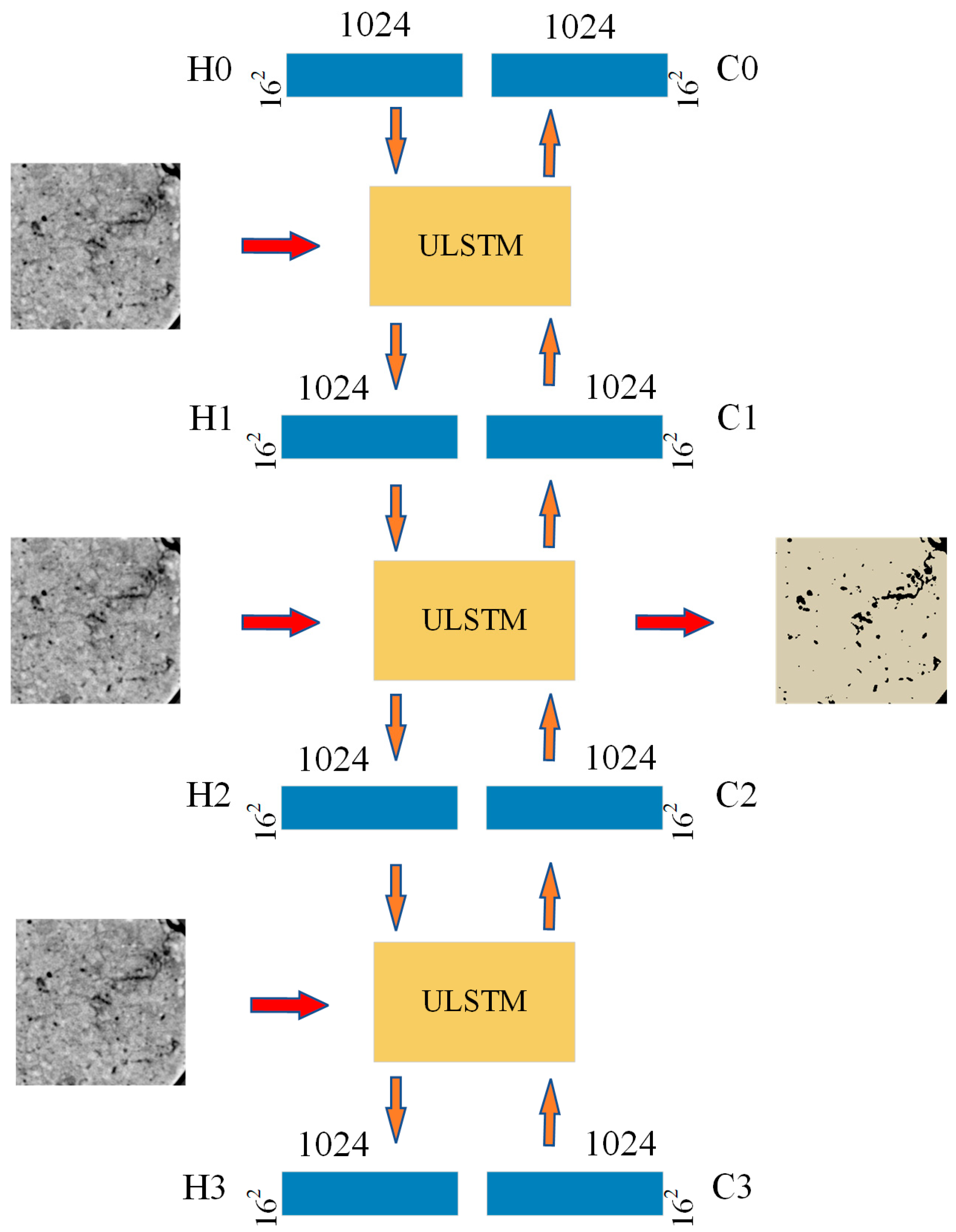
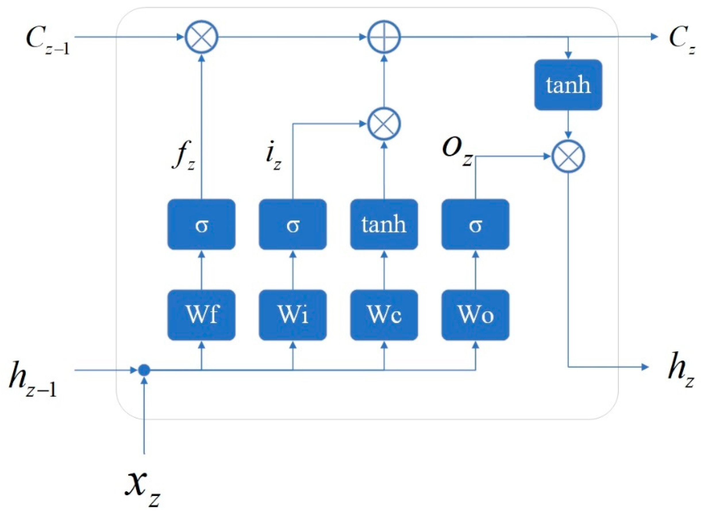
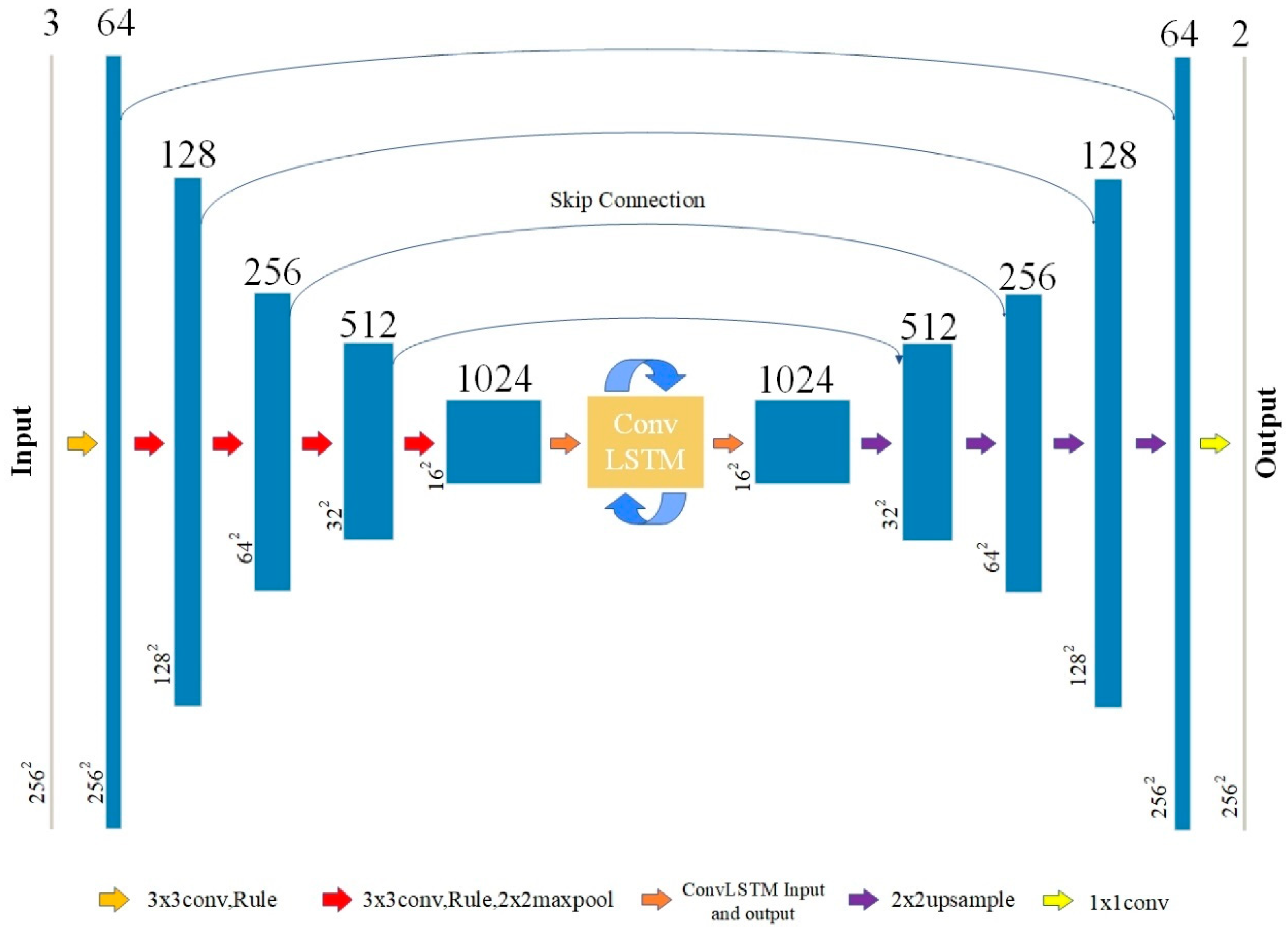
2.2. Neural Network Architecture of the Proposed Method

To enhance the accuracy of soil pore structure identification while preserving the spatial continuity of pores, we propose a novel architecture, the bidirectional U-Net with long short-term memory (BDULSTM). We incorporated a U-Net-based RNN capable of processing multiple inputs concurrently and managing information with the retention and selective forgetting characteristics of an LSTM network. This architecture not only assimilates the spatial information from a sequence of adjacent images but also leverages U-Net’s robust encoding, decoding, and cropping framework to accomplish precise segmentation.

BDULSTM consists of an odd number of ULSTM units, and Figure 1 shows the complete process of data flow and handling within the model when three images are inputted. Each ULSTM unit receives an image as input, with the output of the ULSTM unit positioned in the center designated as the final output of the model. C and H mean the input and output of a cell in ULSTM, respectively, with the numbers indicating the specific cell responsible for transmitting features in the sequence. The sequential representation of soil CT images does not have a before and after order, and each sequential image maintains spatial correlation with its adjacent images. Therefore, by adding one ULSTM unit to each end of the ULSTM unit, a bidirectional structure of ULSTM is formed, namely, bidirectional ULSTM, abbreviated as BDULSTM.

ULSTM is based on the U-Net framework, integrating CLSTM between its encoder and decoder components, as illustrated in Figure 2. The original U-Net network has a U-shaped structure, with the left side downsampling, the right side upsampling, and the middle relying on skip connections to merge the features of each layer in the downsampling with those of each layer in the upsampling. By incorporating the concept of recursion into the foundation of U-Net, ULSTM is capable of processing multiple inputs at once and, like the LSTM network, can preserve and forget certain specific information. It achieves high-precision segmentation by not only integrating the spatial information of several adjacent images but also leveraging the effective coding, decoding, and skip connection structure of the U-Net network.

The ULSTM network architecture utilizes CLSTM with convolutional, pooling, dropout, and deconvolutional layers. The input tensor size is 3 × 256 × 256. First, downsampling of five convolutional and four pooling layers is performed, where the size of the convolution kernel in the convolutional layer associated with each downsampling operation is 3 × 3, with a padding size of one. The numbers of convolution kernels in the layers are 64, 128, 256, 512, and 1024, and the maximum pooling layer dimensions are 2 × 2, with ρ = 0.5 in the dropout layer. The size of the feature tensor is 1024 × 16 × 16 when downsampling is performed. Each CLSTM module contains 1024 hidden units. The convolution kernel size is 5 × 5, the padding size is one, and the output feature tensor size is 1024 × 16 × 16. Four deconvolutional layers are upsampled, where the size of the convolution kernels is 3 × 3, the padding size is one, and the numbers of convolution kernels are 512, 256, 128, and 64, with ρ = 0.5 in the dropout layer. It is worth noting that there is a skip connection between each upsampling and downsampling operation on the same level, allowing the deep and shallow features of the network to be combined to optimize the segmentation accuracy.

In the BDULSTM network architecture, CLSTM provides the ability to fuse features between layers. LSTM is particularly powerful for processing time-series data, but traditional LSTM networks can only process one-dimensional sequence data such as word vectors in natural language processing. To process two-dimensional image sequences, it is necessary to expand a two-dimensional image into one-dimensional sequence data with a data length of width × height to be inputted into the network. However, this method loses much of the information that exists between adjacent pixels in different rows in an image. To address these issues, it is crucial to consider the simplicity and applicability of operations such as convolution and pooling in convolutional neural networks for two-dimensional image processing.

In the pursuit of enhancing the integration of convolutional neural networks and recurrent neural networks with LSTM, Shi et al. (2015) first proposed CLSTM to combine convolutional neural networks and RNNs with LSTM [41]; the architecture of CLSTM is presented in Figure 3 and can be defined as follows:

$$\left\{\begin{array}{l}{i}_z=\sigma \left(x_z\ast W_{xi}+h_{z-1}\ast W_{hi}+b_i\right)\\ f_z=\sigma \left(x_z\ast W_{xf}+h_{z-1}\ast W_{hf}+b_f\right)\\ c_z=c_{z-1}\otimes f_z+i_z\otimes \tanh \left(x_z\ast W_{xc}+h_{z-1}\ast W_{hc}+b_c\right)\\ o_z=\sigma \left(x_z\ast W_{xo}+h_{z-1}\ast W_{ho}+b_o\right)\\ h_z=o_z\otimes \tanh \left(c_z\right)\end{array}\right.$$

(1)

In soil sequence CT slice images, there is no discernible top–down or bottom–up sequential order. Instead, each image is intricately linked to the preceding and succeeding images. In other words, within a soil column slice, the spatial information of a specific slice positioned in the middle is intricately connected to that of the slices positioned below and above the target slice. Therefore, a single CLSTM module is inadequate for capturing complete sequential image information.

To solve this problem, the BDULSTM method was designed with two CLSTM modules to work in conjunction: one forward network to capture the spatial information of a soil column from bottom to top, and one backward network to capture the information from top to bottom. Combining the outputs from both networks yields a set of outputs that seamlessly integrates the spatial context of the soil.

The BDULSTM model demonstrates several key advantages: Firstly, its encode–decode mechanism effectively enhances the ability to extract crucial features from images, thereby improving the recognition of image segmentation details. Secondly, the model has a relatively low total number of parameters, which helps to simplify the training process, reducing the demand for computational resources. Lastly, it can process and analyze multiple image sequences by integrating relevant information from various sequence images to increase the precision and stability of segmentation.

Our method effectively combines the contextual information in soil CT image sequences through its bidirectional structure, allowing for a more comprehensive understanding and utilization of the dynamic changes between images when facing consecutive images. This results in more precise image segmentation in complex scenarios. Such a design not only improves the model’s utilization rate of spatial dimensional information but also provides a new technical approach for image analysis in the soil domain.

2.3. Evaluation Metrics

To evaluate the effect of segmentation quantitatively, the values of soil pores are represented as a positive class, while the values of other soil materials are represented as a negative class. The following four situations form the basis for our evaluation metrics: When a pore is predicted to be a pore, it is recorded as a true positive (TP). When a pore is predicted to be another material, it is recorded as a false negative (FN). Other materials predicted to be pores are recorded as false positives (FP). Other materials predicted to be other materials are recorded as true negatives (TN).

Segmentation accuracy is defined as the proportion of correctly segmented pixels among all pixels in a soil image and can be computed as follows:

$$Acc=\frac{TP+TN}{TP+TN+FP+FN}$$

(2)

Segmentation precision represents the proportion of all correct pore predictions. To some extent, precision can also be defined as the degree of over-segmentation. Precision is computed as follows:

$$P=\frac{TP}{TP+FP}$$

(3)

Segmentation recall represents the proportion of all real soil pores that are correctly identified. To some extent, recall can also be defined as the degree of under-segmentation. Recall is computed as follows:

$$R=\frac{TP}{TP+FN}$$

(4)

For a given soil image, there may be differences in precision and recall, making it inconvenient to compare the advantages and disadvantages of different methods. The F₁-score is the harmonic mean of precision and recall. A higher F₁-score indicates a better model. The F₁-score is computed as follows:

$$F_1=\frac{2\times P\times R}{P+R}=\frac{2TP}{2TP+FP+FN}$$

(5)

3. Results and Discussion

3.1. Experimental Details

To evaluate the performance of different models on the soil pore segmentation task, we evaluated models on a soil CT image dataset containing 3570 soil CT images. The image data were divided into a training set and a test set, at a ratio of 7:3. The training set was used to train all network models, while the test set was used to validate the results of the models. Our model was implemented using the PyTorch framework, and model training was performed using an NVIDIA RTX 2080Ti GPU for acceleration. The model was not spliced into separate components, and an end-to-end training strategy was adopted.

During the training process, the parameters were randomly initialized, the loss function was the weighted cross-entropy loss function, the parameter optimizer was the Adam optimizer, the learning rate was always $lr=1e-5$, and the batch size for batch training was four. The features of adjacent images were added to the LSTM network to produce a beneficial effect for classification, and the number of sequence images affected the model accuracy. For the CLSTM, U-Net–LSTM, and BDULSTM models, we tested inputting three, five, seven, and nine sequential images for training. The soil pore segmentation accuracy, precision, recall, and F₁-score were measured to evaluate the performance of different network models.

3.2. Effects of Different Numbers of Image Slices

Variations in the number of slices in CT images can affect the accuracy and efficiency of models for soil pore recognition tasks. We experimentally compared the performances of models with different numbers of CT image slices and analyzed the differences in the results.

BDULSTM utilizes a bidirectional architecture to leverage the forward and backward features of adjacent images. Therefore, the number of sequential images affects the theoretical results of the model. Different numbers of input sequence images were tested for the three soil samples (i.e., three, five, seven, and nine images).

As shown in

Table 1. Quantitative comparisons of segmentation performance (%).

Soil Type	Number of Images	Accuracy	Precision	Recall	F1-Score
Primary	3	96.51 ± 1.02 × 10−2	96.54 ± 1.55 × 10−2	68.02 ± 7.54 × 10−1	79.48 ± 2.93 × 10−1
	5	96.47 ± 1.15 × 10−2	98.23 ± 9.25 × 10−3	66.37 ± 8.28 × 10−1	78.85 ± 3.53 × 10−1
	7	96.49 ± 1.01 × 10−2	96.40 ± 1.45 × 10−2	67.96 ± 7.64 × 10−1	79.38 ± 2.92 × 10−1
	9	96.48 ± 1.07 × 10−2	96.83 ± 1.31 × 10−2	67.51 ± 8.03 × 10−1	79.20 ± 3.17 × 10−1
Frozen	3	98.72 ± 3.44 × 10−3	96.59 ± 8.08 × 10−2	86.80 ± 7.93 × 10−1	91.08 ± 1.68 × 10−1
	5	98.88 ± 1.11 × 10−3	93.49 ± 2.16 × 10−1	92.15 ± 4.51 × 10−1	92.50 ± 5.08 × 10−2
	7	98.80 ± 9.14 × 10−4	92.08 ± 3.08 × 10−1	92.76 ± 4.05 × 10−1	92.07 ± 4.25 × 10−2
	9	98.87 ± 1.40 × 10−3	94.08 ± 2.29 × 10−1	91.48 ± 5.40 × 10−1	92.40 ± 6.85 × 10−2
Thawed	3	98.93 ± 2.94 × 10−3	90.74 ± 1.90 × 10−1	92.68 ± 6.16 × 10−1	91.46 ± 1.76 × 10−1
	5	98.89 ± 3.03 × 10−3	90.11 ± 1.97 × 10−1	92.74 ± 6.14 × 10−1	91.17 ± 1.80 × 10−1
	7	98.95 ± 3.03 × 10−3	90.83 ± 2.05 × 10−1	92.85 ± 6.09 × 10−1	91.59 ± 1.81 × 10−1
	9	98.78 ± 3.28 × 10−3	88.30 ± 2.28 × 10−1	93.02 ± 6.09 × 10−1	90.37 ± 1.91 × 10−1

, both accuracy and F₁-score improve slightly with an increase in the number of sequence images. Although the improvement is slight, the variance tends to decrease, corresponding to increased robustness. However, the number of sequence images and evaluation indicators do not exhibit linear relationships. When the number of images increased from seven to nine, the evaluation indicators no longer improved. CLSTM has a bottleneck in terms of sequence processing power, meaning excessively long sequences lead to degraded performance. The qualitative results for different numbers of images can be found in Figure 4.

A previous study on pulmonary nodule classification using CT scans found that using additional slices could capture more comprehensive information regarding nodule characteristics, leading to a higher performance [42]. However, there may be a limit to the benefit of adding more slices, as the computational complexity of the model may increase, leading to issues such as overfitting. Increasing the number of sequence images had a positive effect on model performance, but the training time also increased and model performance stopped improving when the number of sequence images increased to nine. Therefore, groups of seven images were selected as BDULSTM sequences based on the results of this experiment. The results of our analysis provide insights into the optimal number of slices required for pore recognition and contribute to the advancement of CT image analysis.

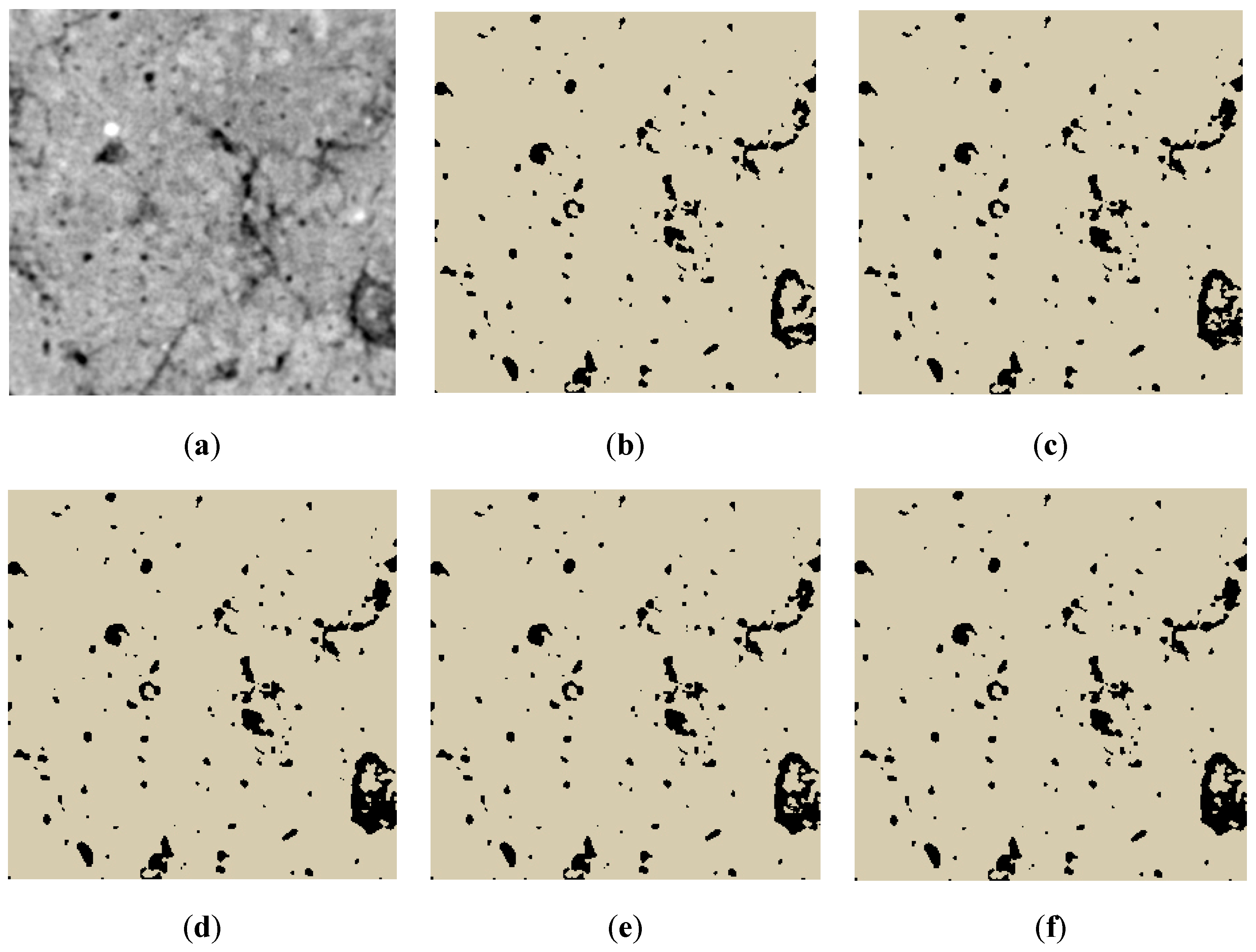
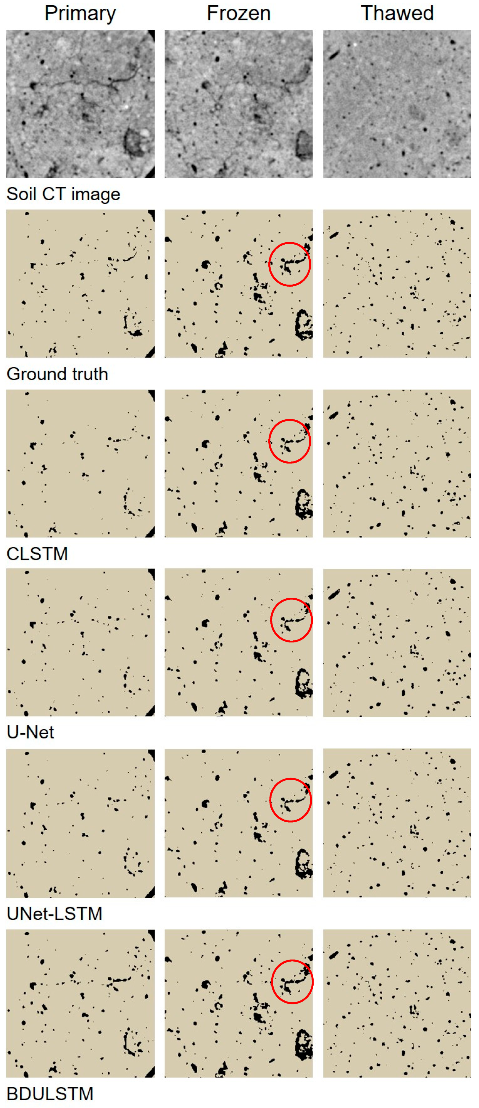
3.3. Qualitative Results

In the original CT images of soil, pores appeared as black regions, signifying areas of interest for segmentation. Other soil constituents, such as solid particles, were represented in shades of gray and white. Figure 5 illustrates the segmentation outcomes from various network models. Although the results from the majority of the models are predominantly precise, a number of them tend to underestimate the pore size to different extents when contrasted with images that have been manually adjusted. Given the variability in soil composition and the heterogeneity of pore distributions, numerous gray values within the soil CT images may confound the models’ assessments.

Certain small pores are not well segmented and are predominantly overlooked, which can be ascribed in part to the diminished representation of pore structures in the soil images. The absent pores are denoted by circles in Figure 5. For elongated, strip-shaped pores, only the proposed method successfully connects them in a manner akin to the calibration chart, whereas alternative methods yield fragmented results. Qualitatively, the experimental outcomes suggest that BDULSTM offers superior segmentation, capturing the smallest pores and providing results that visually approximate those of the manually refined images most closely.

3.4. Quantitative Evaluations

As shown in

Table 2. Quantitative comparisons of segmentation performance (%).

Model	Soil Type	Accuracy	Precision	Recall	F1-Score
CLSTM	Primary	96.56 ± 9.35 × 10−3	93.40 ± 3.50 × 10−1	71.94 ± 1.31	80.45 ± 3.10 × 10−1
	Frozen	97.79 ± 7.12 × 10−3	99.10 ± 9.05 × 10−3	61.92 ± 2.74	74.89 ± 1.61
	Thawed	97.71 ± 8.16 × 10−3	99.88 ± 2.80 × 10−4	63.79 ± 1.87	77.04 ± 9.82 × 10−1
U-Net	Primary	96.57 ± 1.19 × 10−2	94.66 ± 4.33 × 10−1	70.88 ± 3.19 × 10−1	80.20 ± 1.48
	Frozen	97.28 ± 1.85 × 10−2	74.79 ± 2.86 × 10−1	99.55 ± 6.44 × 10−1	85.16 ± 7.31 × 10−3
	Thawed	98.47 ± 4.59 × 10−3	99.94 ± 2.31 × 10−1	77.73 ± 4.89 × 10−4	87.25 ± 5.80 × 10−1
U-Net–LSTM	Primary	96.57 ± 1.57 × 10−2	96.95 ± 1.37 × 10−1	68.86 ± 1.69	79.67 ± 6.32 × 10−1
	Frozen	98.43 ± 1.08 × 10−2	98.71 ± 1.68 × 10−2	73.03 ± 3.88	82.38 ± 1.70
	Thawed	98.50 ± 7.46 × 10−3	99.65 ± 4.95 × 10−3	76.49 ± 1.92	85.84 ± 7.24 × 10−1
BDULSTM	Primary	96.49 ± 1.01 × 10−2	96.40 ± 1.45 × 10−2	67.96 ± 7.64 × 10−1	79.38 ± 2.92 × 10−1
	Frozen	98.80 ± 9.14 × 10−4	92.08 ± 3.08 × 10−1	92.76 ± 4.05 × 10−1	92.07 ± 4.25 × 10−2
	Thawed	98.95 ± 3.03 × 10−3	90.83 ± 2.05 × 10−1	92.85 ± 6.09 × 10−1	91.59 ± 1.81 × 10−1

, CLSTM yielded the lowest accuracy and the highest variance. The poor performance of CLSTM can be attributed to the fact that it simply switches the processes within LSTM to convolutions for 2D data, rather than being properly tuned for image segmentation. The accuracy values of the other models are high and similar, and the variance of BDULSTM is the smallest among all models, demonstrating that its performance is the most stable. The variance further decreases for U-Net–LSTM and BDULSTM when increasing the number of sequence images, indicating that increasing the number of sequence images is beneficial for accuracy.

CLSTM achieved the greatest precision of 0.98. However, it had an extremely poor recall rate. This indicates that CLSTM is under-segmented and loses a portion of the soil pore region, resulting in worse performance than U-Net. As U-Net–LSTM and BDULSTM progressed from three sequence images to seven sequence images, their precision decreased, indicating that larger pore structures were obtained. Correspondingly, their recall increased following the addition of sequence images. This indicates that adding more sequence images causes these models to correct for omissions in segmenting pores and to classify more regions as pores.

The F₁-score, which is a combined precision and recall evaluation indicator, is the most comprehensive measure of segmentation effect. The F₁-score of CLSTM was the lowest, indicating that its segmentation effect was the worst. BDULSTM slightly outperformed U-Net–LSTM, and after increasing from three to seven sequence images its F₁-score increased significantly, further demonstrating that increasing the number of sequence images is effective up to a certain point.

In general, CLSTM is not suitable for directly segmenting images. U-Net performed well in general, but it had some limitations. Additionally, U-Net–LSTM is beneficial for U-Net optimization. All indicators of BDULSTM were the best and exhibited the smallest variance, indicating that it has strong robustness and adaptability for identifying pores and solid particles in complex soils.

3.5. Neural Network Complexity

In

Table 3. Comparison of number of parameters, FLOPs, and memory requirements for various models.

Models	Parameters (M)	FLOPs (G)	Memory (M)
CLSTM	0.55	10.85	32.87
U-Net	7.41	11.60	202.75
U-Net–LSTM	51.90	38.47	442.50
BDULSTM	50.82	32.87	409.50

, we present the numbers of parameters, FLOPs, and memory sizes of the models. The FLOPs and memory size were calculated based on the input size of 3 × 256 × 256 using the sliding window method. There were seven sequence images for CLSTM, U-Net–LSTM, and BDULSTM. According to our benchmarks, BDULSTM is a moderately sized model, with 50.82 M parameters and 32.87 GFLOPs. For comparison, U-Net–LSTM has 51.90 M parameters and 38.47 GFLOPs.

Although more complex than both the basic CLSTM and U-Net, BDULSTM has lower model complexity than U-Net–LSTM and exhibited better performance on our benchmarks. Additionally, the memory size of BDULSTM is 409.50 M, while that of U-Net–LSTM is 442.50 M. Therefore, BDULSTM requires less memory than U-Net–LSTM to process sequence images.

4. Conclusions

Our study successfully employed the BDULSTM method for 3D segmentation of soil CT images, leveraging the combined strengths of U-Net and CLSTM networks to process image sequences and improve segmentation performance. Experiments on soil CT images in various freeze–thaw scenarios yielded the following conclusions:

(1) The performance of BDULSTM varies depending on the number of sequence images used. The maximum performance is achieved when utilizing seven images.

(2) BDULSTM effectively captures the 3D structure of soil pores by processing sequential images. When compared to other models, BDULSTM demonstrates superior performance in pore segmentation.

(3) The model complexity, floating-point operations (FLOPs), and memory requirements of BDULSTM remain reasonably low, thereby expanding the practical application of the BDULSTM method and facilitating its operation on low-power devices.

When processing complex 3D data that heavily depend on spatial structures, BDULSTM may not perform as well as 3D convolutional networks. However, if computational resources are extremely limited, using BDULSTM could be a reasonable compromise. In conclusion, BDULSTM has shown promising capabilities in segmenting 3D soil pore structures within CT images, and it lays a solid groundwork for further 3D pore structure analysis in soil science.

References

1. Borrelli, P.; Robinson, D.A.; Panagos, P.; Lugato, E.; Yang, J.E.; Alewell, C.; Wuepper, D.; Montanarella, L.; Ballabio, C. Land use and climate change impacts on global soil erosion by water (2015–2070). Proc. Natl. Acad. Sci. USA 2020, 117, 21994–22001. [Google Scholar] [CrossRef] [PubMed]
2. Baveye, P.C.; Balseiro-Romero, M.; Bottinelli, N.; Briones, M.; Capowiez, Y.; Garnier, P.; Kravchenko, A.; Otten, W.; Pot, V.; Schlüter, S. Lessons from a landmark 1991 article on soil structure: Distinct precedence of non-destructive assessment and benefits of fresh perspectives in soil research. Soil Res. 2022, 60, 321–336. [Google Scholar] [CrossRef]
3. Haubitz, B.; Prokop, M.; Döhring, W.; Ostrom, J.; Wellnhofer, P. Computed tomography of Archaeopteryx. Paleobiology 1988, 14, 206–213. [Google Scholar] [CrossRef]
4. Xiong, P.; Zhang, Z.; Hallett, P.D.; Peng, X. Variable responses of maize root architecture in elite cultivars due to soil compaction and moisture. Plant Soil 2020, 455, 79–91. [Google Scholar] [CrossRef]
5. Zhang, T.; Liu, Q.; Wang, X.; Ji, X.; Du, Y. A 3D reconstruction method of porous media based on improved WGAN-GP. Comput. Geosci. 2022, 165, 105151. [Google Scholar] [CrossRef]
6. Zhao, Z.; Zhou, X.-P. An integrated method for 3D reconstruction model of porous geomaterials through 2D CT images. Comput. Geosci. 2019, 123, 83–94. [Google Scholar] [CrossRef]
7. Pereira, M.F.L.; Cruvinel, P.E. A model for soil computed tomography based on volumetric reconstruction, Wiener filtering and parallel processing. Comput. Electron. Agric. 2015, 111, 151–163. [Google Scholar] [CrossRef]
8. Xu, J.; Ren, C.; Wang, S.; Gao, J.; Zhou, X. Permeability and microstructure of a saline intact loess after dry-wet cycles. Adv. Civil Eng. 2021, 2021, 6653697. [Google Scholar] [CrossRef]
9. Zhang, X.; Neal, A.L.; Crawford, J.W.; Bacq-Labreuil, A.; Akkari, E.; Rickard, W. The effects of long-term fertilizations on soil hydraulic properties vary with scales. J. Hydrol. 2021, 593, 125890. [Google Scholar] [CrossRef] [PubMed]
10. Gattullo, C.E.; Allegretta, I.; Porfido, C.; Rascio, I.; Spagnuolo, M.; Terzano, R. Assessing chromium pollution and natural stabilization processes in agricultural soils by bulk and micro X-ray analyses. Environ. Sci. Pollut. Res. 2020, 27, 22967–22979. [Google Scholar] [CrossRef] [PubMed]
11. Scotson, C.P.; Duncan, S.J.; Williams, K.A.; Ruiz, S.A.; Roose, T. X-ray computed tomography imaging of solute movement through ridged and flat plant systems. Eur. J. Soil Sci. 2021, 72, 198–214. [Google Scholar] [CrossRef]
12. Tang, C.-S.; Lin, L.; Cheng, Q.; Zhu, C.; Wang, D.-W.; Lin, Z.-Y.; Shi, B. Quantification and characterizing of soil microstructure features by image processing technique. Comput. Geotech. 2020, 128, 103817. [Google Scholar] [CrossRef]
13. Meng, C.; Niu, J.; Yu, H.; Du, L.; Yin, Z. Research progress in influencing factors and measuring methods of three-dimensional characteristics of soil macropores. J. Beijing For. Univ. 2020, 42, 9–16. [Google Scholar]
14. Karimpouli, S.; Tahmasebi, P. Segmentation of digital rock images using deep convolutional autoencoder networks. Comput. Geosci. 2019, 126, 142–150. [Google Scholar] [CrossRef]
15. Tempelaere, A.; Phan, H.M.; Van De Looverbosch, T.; Verboven, P.; Nicolai, B. Non-destructive internal disorder segmentation in pear fruit by X-ray radiography and AI. Comput. Electron. Agric. 2023, 212, 108142. [Google Scholar] [CrossRef]
16. Van De Looverbosch, T.; Vandenbussche, B.; Verboven, P.; Nicolaï, B. Nondestructive high-throughput sugar beet fruit analysis using X-ray CT and deep learning. Comput. Electron. Agric. 2022, 200, 107228. [Google Scholar] [CrossRef]
17. Xiberta, P.; Boada, I.; Bardera, A.; Font-i-Furnols, M. A semi-automatic and an automatic segmentation algorithm to remove the internal organs from live pig CT images. Comput. Electron. Agric. 2017, 140, 290–302. [Google Scholar] [CrossRef]
18. Litjens, G.; Kooi, T.; Bejnordi, B.E.; Setio, A.A.A.; Ciompi, F.; Ghafoorian, M.; Van Der Laak, J.A.; Van Ginneken, B.; Sánchez, C.I. A survey on deep learning in medical image analysis. Med. Image Anal. 2017, 42, 60–88. [Google Scholar] [CrossRef] [PubMed]
19. Shen, D.; Wu, G.; Suk, H.-I. Deep learning in medical image analysis. Annu.Rev. Biomed. Eng. 2017, 19, 221–248. [Google Scholar] [CrossRef] [PubMed]
20. Wieland, R.; Ukawa, C.; Joschko, M.; Krolczyk, A.; Fritsch, G.; Hildebrandt, T.B.; Schmidt, O.; Filser, J.; Jimenez, J.J. Use of deep learning for structural analysis of computer tomography images of soil samples. R. Soc. Open Sci. 2021, 8, 201275. [Google Scholar] [CrossRef] [PubMed]
21. Wang, H.; Li, Y.; Zhang, H.; Meng, D.; Zheng, Y. InDuDoNet+: A deep unfolding dual domain network for metal artifact reduction in CT images. Med. Image Anal. 2023, 85, 102729. [Google Scholar] [CrossRef] [PubMed]
22. Dutta, S.; Nwigbo, K.T.; Michetti, J.; Georgeot, B.; Pham, D.H.; Kouamé, D.; Basarab, A. Computed Tomography Image Restoration Using a Quantum-Based Deep Unrolled Denoiser and a Plug-and-Play Framework. In Proceedings of the 2023 31st European Signal Processing Conference (EUSIPCO), Helsinki, Finland, 4–8 September 2023; pp. 845–849. [Google Scholar]
23. Saxena, N.; Day-Stirrat, R.J.; Hows, A.; Hofmann, R. Application of deep learning for semantic segmentation of sandstone thin sections. Comput. Geosci. 2021, 152, 104778. [Google Scholar] [CrossRef]
24. Liang, J.; Sun, Y.; Lebedev, M.; Gurevich, B.; Nzikou, M.; Vialle, S.; Glubokovskikh, S. Multi-mineral segmentation of micro-tomographic images using a convolutional neural network. Comput. Geosci. 2022, 168, 105217. [Google Scholar] [CrossRef]
25. Han, Q.; Zhao, Y.; Liu, L.; Chen, Y.; Zhao, Y. A simplified convolutional network for soil pore identification based on computed tomography imagery. Soil Sci. Soc. Am. J. 2019, 83, 1309–1318. [Google Scholar] [CrossRef]
26. Bai, H.; Liu, L.; Han, Q.; Zhao, Y.; Zhao, Y. A novel UNet segmentation method based on deep learning for preferential flow in soil. Soil Till. Res. 2023, 233, 105792. [Google Scholar] [CrossRef]
27. Ronneberger, O.; Fischer, P.; Brox, T. U-net: Convolutional networks for biomedical image segmentation. In Proceedings of the Medical Image Computing and Computer-Assisted Intervention–MICCAI 2015: 18th International Conference, Munich, Germany, 5–9 October 2015; Proceedings, Part III 18. pp. 234–241. [Google Scholar]
28. Zhang, Y.; He, Z.; Jiang, R.; Liao, L.; Meng, Q. Improved Computer Vision Framework for Mesoscale Simulation of Xiyu Conglomerate Using the Discrete Element Method. Appl. Sci. 2023, 13, 13000. [Google Scholar] [CrossRef]
29. Roslin, A.; Marsh, M.; Provencher, B.; Mitchell, T.; Onederra, I.; Leonardi, C. Processing of micro-CT images of granodiorite rock samples using convolutional neural networks (CNN), Part II: Semantic segmentation using a 2.5 D CNN. Miner. Eng. 2023, 195, 108027. [Google Scholar] [CrossRef]
30. Phan, J.; Ruspini, L.C.; Lindseth, F. Automatic segmentation tool for 3D digital rocks by deep learning. Sci. Rep. 2021, 11, 19123. [Google Scholar] [CrossRef] [PubMed]
31. Çiçek, Ö.; Abdulkadir, A.; Lienkamp, S.S.; Brox, T.; Ronneberger, O. 3D U-Net: Learning dense volumetric segmentation from sparse annotation. In Proceedings of the Medical Image Computing and Computer-Assisted Intervention–MICCAI 2016: 19th International Conference, Athens, Greece, 17–21 October 2016; Proceedings, Part II 19. pp. 424–432. [Google Scholar]
32. Vu, M.H.; Grimbergen, G.; Simkó, A.; Nyholm, T.; Löfstedt, T. End-to-End Cascaded U-Nets with a Localization Network for Kidney Tumor Segmentation. arXiv 2019, arXiv:1910.07521. [Google Scholar]
33. Milletari, F.; Navab, N.; Ahmadi, S.-A. V-net: Fully convolutional neural networks for volumetric medical image segmentation. In Proceedings of the 2016 Fourth International Conference on 3D Vision (3DV), Stanford, CA, USA, 25–28 October 2016; pp. 565–571. [Google Scholar]
34. Kitrungrotsakul, T.; Iwamoto, Y.; Han, X.-H.; Takemoto, S.; Yokota, H.; Ipponjima, S.; Nemoto, T.; Wei, X.; Chen, Y.-W. A cascade of CNN and LSTM network with 3D anchors for mitotic cell detection in 4D microscopic image. In Proceedings of the ICASSP 2019—2019 IEEE International Conference on Acoustics, Speech and Signal Processing (ICASSP), Brighton, UK, 12–17 May 2019; pp. 1239–1243. [Google Scholar]
35. Novikov, A.A.; Major, D.; Wimmer, M.; Lenis, D.; Bühler, K. Deep sequential segmentation of organs in volumetric medical scans. IEEE Trans. Med. Imaging 2018, 38, 1207–1215. [Google Scholar] [CrossRef]
36. Stollenga, M.F.; Byeon, W.; Liwicki, M.; Schmidhuber, J. Parallel multi-dimensional LSTM, with application to fast biomedical volumetric image segmentation. In Proceedings of the 28th International Conference on Neural Information Processing Systems, Montreal, QC, Canada, 7–12 December 2015; Volume 28. [Google Scholar]
37. Chen, J.; Yang, L.; Zhang, Y.; Alber, M.; Chen, D.Z. Combining fully convolutional and recurrent neural networks for 3d biomedical image segmentation. In Proceedings of the 30th International Conference on Neural Information Processing Systems, Barcelona, Spain, 5–12 December 2016; Volume 29. [Google Scholar]
38. Ganaye, P.-A.; Sdika, M.; Triggs, B.; Benoit-Cattin, H. Removing segmentation inconsistencies with semi-supervised non-adjacency constraint. Med. Image Anal. 2019, 58, 101551. [Google Scholar] [CrossRef] [PubMed]
39. Wang, E.; Zhao, Y.; Xia, X.; Chen, X. Effects of freeze-thaw cycles on black soil structure at different size scales. Acta Ecol. Sin. 2014, 34, 6287–6296. [Google Scholar]
40. Zhao, Y.; Han, Q.; Zhao, Y.; Liu, J. Soil pore identification with the adaptive fuzzy C-means method based on computed tomography images. J. For. Res. 2019, 30, 1043–1052. [Google Scholar] [CrossRef]
41. Shi, X.; Chen, Z.; Wang, H.; Yeung, D.-Y.; Wong, W.-K.; Woo, W.-C. Convolutional LSTM network: A machine learning approach for precipitation nowcasting. In Proceedings of the 28th International Conference on Neural Information Processing Systems, Montreal, QC, Canada, 7–12 December 2015; Volume 28. [Google Scholar]
42. Candemir, S.; Jaeger, S.; Palaniappan, K.; Musco, J.P.; Singh, R.K.; Xue, Z.; Karargyris, A.; Antani, S.; Thoma, G.; McDonald, C.J. Lung segmentation in chest radiographs using anatomical atlases with nonrigid registration. IEEE Trans. Med. Imaging 2013, 33, 577–590. [Google Scholar] [CrossRef] [PubMed]
Figure 1. BDULSTM architecture.
Applsci 14 03352 g001
Figure 2. Internal architecture of ULSTM cells.
Applsci 14 03352 g002
Figure 3. Internal architecture of CLSTM cells.
Applsci 14 03352 g003
Figure 4. Qualitative comparison of different numbers of sequence images: (a) original soil CT image, (b) ground truth, (c) three images in sequence, (d) five images in sequence, (e) seven images in sequence, and (f) nine images in sequence.
Applsci 14 03352 g004
Figure 5. Qualitative comparison of different models, where rows represent different models and columns represent different conditions.
Applsci 14 03352 g005