Comparative Analysis of Machine Learning Methods for Predicting Energy Recovery from Waste

Abstract

In the context of escalating energy demands and the quest for sustainable waste management solutions, this paper evaluates the efficacy of three machine learning methods—ElasticNet, Decision Trees, and Neural Networks—in predicting energy recovery from municipal waste across the European Union. As renewable energy sources increasingly dominate the energy production landscape, the integration of Waste-to-Energy (WTE) processes presents a dual advantage: enhancing waste management and contributing to the renewable energy mix. This study leverages a dataset incorporating economic and environmental indicators from 25 European countries, spanning 2013–2020, to compare the predictive capabilities of the three machine learning models. The analysis reveals that Neural Networks, with their intricate pattern recognition capabilities, outperform ElasticNet and Decision Trees in predicting energy recovery metrics, as evidenced by superior performance in key statistical indicators such as R-value, Mean Squared Error (MSE), and Mean Absolute Error (MAE). The comparative analysis not only demonstrates the effectiveness of each method but also suggests Neural Networks as a pivotal tool for informed decision-making in waste management and energy policy formulation. Through this investigation, the paper contributes to the sustainable energy and waste management discourse, emphasizing the critical intersection of advanced technologies, policy considerations, and environmental stewardship in addressing contemporary energy challenges.

1. Introduction

Energy is a fundamental element for the functioning of contemporary society, and the laws governing its use have both economic and strategic-political implications. The objective of the European Union’s energy policy is to decrease reliance on imported energy and energy products by encouraging the implementation of energy-saving measures and the inclusion of renewable energy sources (RES) [1]. Acquiring energy relies on various sources that vary by country. In 2021, renewable energy was the primary source of energy production in the European Union, accounting for 41% of total production. Solid fuels (18%), natural gas (6%), and oil (3%) also contributed to energy production [2]. Energy production in EU countries is highly diverse. In Poland, Estonia, and the Czech Republic, solid fuels are the primary source of energy production accounting for 70.7%, 50%, and 53.60% of total electricity production, respectively [3]. However, Norway and Sweden have a significant share of renewable energy, with 73% and 55%, respectively. Norway is renowned for its use of hydropower, which accounted for 81% of renewable energy sources in 2018. In contrast, Sweden is known for its production of wind energy, which accounted for 20%. Finland utilizes biomass for both heating and power generation, with 79% of its renewable energy coming from this source [4]. Global energy consumption has been increasing annually by an average of 1% to 2% for over half a century. European Union (EU) countries are seeking innovative and sustainable solutions to improve waste management and energy efficiency in response to the growing demand for energy and the ongoing challenge of municipal waste. One promising direction is the conversion of municipal waste to energy. This approach reduces the amount of waste reaching landfills and produces energy. It objectively assesses the potential benefits of this approach [5].

The conversion of municipal waste to energy, known as Waste-to-Energy (WTE), not only aids in waste management but also contributes to the production of renewable energy and reduces greenhouse gas emissions by replacing solid fuels. WTE encompasses combustion, pyrolysis, gasification, and methane fermentation. It enables the production of energy from municipal waste that would otherwise be sent to landfills, thus diversifying energy sources and increasing energy security [6]. The conversion of municipal waste to energy has several advantages. However, this process also presents various challenges and issues. Technological advancements are closely linked to the environmental and economic policies of individual countries and global trends in sustainable development [7].

The variable composition and calorific value of municipal waste pose significant challenges for converting waste into energy [8]. Installations must be designed in a way that enables them to cope with the volatility of the composition and fuel value of waste. This requires the use of advanced processing technologies, such as waste-free systems and exhaust gas purification technology, to minimize pollution emissions [9]. To enhance energy and economic efficiency, waste-to-energy plants can implement several strategies. These include accurate waste segregation at the source stage, pre-processing (such as drying to reduce waste moisture and increase calorific value), and mixing waste streams of varying fuel value to achieve a more stable and optimal combustion mixture [10].

Constructing and maintaining energy processing plants, particularly waste-to-energy facilities, presents a significant challenge due to the substantial investments required. Availability of these facilities can help reduce the complexity of technology and high maintenance costs, particularly in regions with limited financial resources. Therefore, decision-making regarding the implementation of such solutions requires careful assessment of profitability as well as consideration of all arguments for and against. Mathematical models can improve the process of estimating the energy potential of municipal waste, making environmental decisions more effective and based on solid analytical foundations.

Machine learning models need to be created based on various sets of data, including economic and environmental research, to ensure their generalization. Research on learning techniques and model adaptation can provide ways to overcome restrictions in the use of waste transformation methods. These models can optimize processes to achieve higher efficiency, resulting in increased energy recovery indicators.

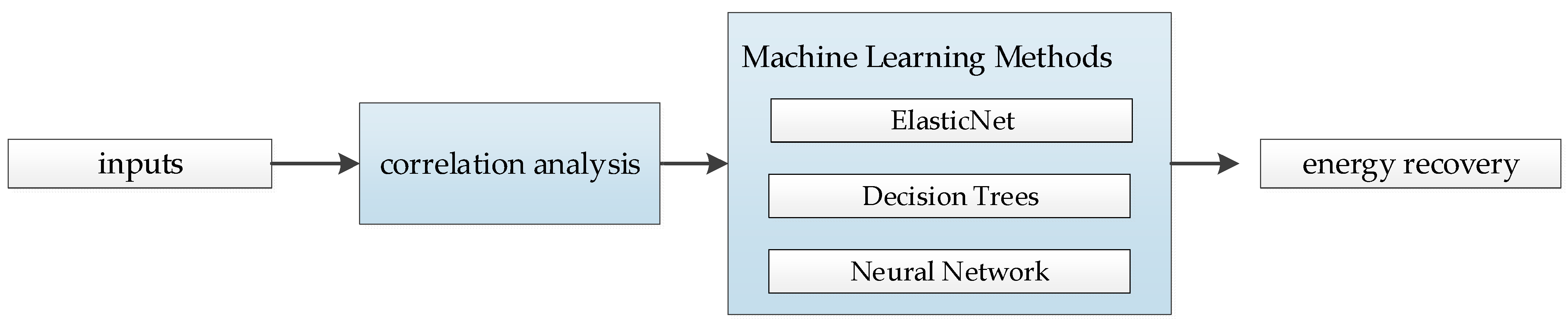
The application of machine learning methods like ElasticNet, Decision Trees, and Neural Networks to model energy recovery from waste in European Union countries is an approach that leverages diverse economic and environmental indicators to predict and optimize energy recovery processes. The use of such comprehensive input data—including electricity prices by type of user, energy productivity, final energy consumption, GDP at market prices, recycling rates of municipal waste, domestic material consumption per capita, environmental tax revenue, and the share of energy from renewable sources—ensures a broad and nuanced understanding of the factors influencing energy recovery from waste.

Mathematical models can be used to identify efficient and sustainable methods of transforming waste into energy, thereby reducing the amount of waste sent to landfills. Machine learning models, with their adaptability, can forecast future trends and changes in factors affecting energy recovery. This predictive ability is crucial for planning and adapting sustainable development strategies.

1.1. Literature Review

Mathematical models can be used to forecast the amount of waste and the amount of energy produced based on various, often non-linear, factors affecting the combustion or fermentation process of municipal waste. Various machine learning models were used, including artificial neural networks (ANNs), regression trees, multi-dimensional adaptive regression, random forest, the theory of roughing harvest, reinforced regression, and combined methods for forecasting the amount of municipal waste.

Yang et al. (2021) conducted a comparison of six machine learning models for municipal solid waste prediction (MSW) in China [11]. The models included Multiple Linear Regression (MLR), Support Vector Regression (SVR), Random Forest (RF), Extreme Gradient Boosting (XGBOOST), K-Nearest Neighbor (KNN), and Artificial Neural Network. The study also examined the correlation between variables based on past entries. The results confirm high prediction accuracy for all machine learning models, with the ANN model performing the best. The data include Total Regional Gross Domestic Product (GDP), Value Added by Transportation, Warehouse, and Postal Services, Wholesale and Retail Value Added, Value Added by the Accommodation and Catering Industry, City Area, Urban Population Density, the Number of Urban Populations, Urban Per Capita Disposable Income, and Total Retail Sales of Consumer Goods. The regional GDP indicator is widely acknowledged as the most significant variable in predicting waste production [11]. In the authors’ previous study, a Neural Network was employed for predicting the volume of municipal solid waste in Poland. Kulisz and Kujawska utilized neural network modeling to estimate the quantities of MSW in Poland, categorizing the waste into five types: glass, biodegradable materials, paper and cardboard, plastics and metals, and other assorted waste [12]. The proposed models integrated various explanatory variables to assess the impact of economic, demographic, and social factors on waste generation volumes. The neural network models varied by adjusting the number of hidden neurons between 2 and 10. The performance of these models was evaluated based on the Pearson correlation coefficient (R) and the mean squared error (MSE). The ANN model featuring six hidden neurons demonstrated high predictive accuracy, evidenced by a significant R-value (0.914) for the categorized waste types. When analyzing statistical data from 2013 to 2019, it was found that, the model predicted a 2% increase in waste production by 2024. These results confirm the efficiency of the ANN model as a cost-effective approach for designing integrated waste management systems [12].

A significant parameter for waste energy assessment is the chemical properties of waste, particularly the Higher Heating Value (HHV). Waste used to obtain energy must be characterized by a high HHV [13]. Determining the higher heating value of waste can be challenging due to the heterogeneity of the material and the precision of measuring methods. This can make it difficult to obtain accurate and representative results. Advanced analytical methods are required due to differences in humidity, chemical composition, and waste pollution. Prior to designing installations for efficient and optimized waste processing, it is advisable to create mathematical models to forecast the higher fuel value of waste. Accurate HHV forecasting enables minimization of waste directed to landfills by facilitating effective energy utilization. Models also aid in identifying waste with the highest energy value, thereby enabling better selection and segregation of materials prior to processing. Accurate forecasting of the higher heating value enables adjustment of combustion process parameters, including temperature, air flow, or combustion time. This enhances energy efficiency and reduces harmful substance emissions [14]. Several studies have developed models to estimate HHV accurately for various types of MSW. Jose and Sasipraba (2023) compared various models for HHV forecasting, including multiple linear regression (MLR), genetic programming (GP), elastic reverse propagation (RP), Levenberg Marquardt (LM), and Deep Support Vector Machine (DSVM), as well as Optimal Deep Learning-Based HHV Prediction (ODL-HHVP), to identify the most accurate method [15]. The input data consisted of the content of oxygen, water, hydrogen, carbon, nitrogen, sulfur, and ash in waste. The study found that ODL-HHVP was the most accurate method for HHV forecasting [15]. Bagheri et al. (2019) conducted a study to compare the accuracy of three models—programming of gene expression (GEP), support vector machine (SVM), and the Feed-Forward neural network (FFNN)—in predicting HHV. The input data used were the content of C, H, N, and S in municipal waste. The statistical performance of the developed GEP, SVM, and FFNN models for R2 were 0.966, 0.973, and 0.978, respectively, and for RMSE were 1.57, 1.44, and 1.25, respectively [6]. In the authors’ previous studies, a machine learning model for HHV prediction of different types of biomass was developed [16]. The input data used were the results of elemental biomass analysis, carbon, nitrogen, and hydrogen analysis. The best results were obtained for a neural network with three input neurons and nine hidden layer neurons. The model was characterized by r = 0.988 and MSE = 0.3. The research has shown that the ANN model can estimate the HHV value based on the elemental composition of the biomass. The models that use waste chemical analyses as input data are presented above. These models are employed to develop and optimize specific waste processing technologies [16].

In addition to the models based on physical and chemical analysis, it is possible to create models based on energy statistics. Statistical models enable large-scale analysis and forecasting, covering entire energy systems, economic sectors, or regions. The models based on statistics enable easy integration with other types of data, such as economic growth, changes in energy policy, or trends in waste production [17]. This provides a broader understanding of the impact of these factors on the energy potential of waste. Statistical models are also more adaptable to changing trends, new processing technologies, or environmental policy changes, which is particularly important in the rapidly evolving waste management and energy sectors. Statistical models are frequently used to support political and strategic decisions. They provide the information necessary for infrastructure planning, investments in energy recovery technologies, and sustainable development policies. Decision-makers and energy planners can use them to develop long-term strategies for waste and energy management, identifying potential growth and investment areas.

Machine learning models are also used to forecast energy efficiency and waste drilling efficiency. In a comparative study conducted by Meerasri and Sothornvit (2022), mathematical models, multiple linear regression, and artificial neural networks (ANNs) were used to predict humidity ratio and drying speed of pineapple cubes. The ANN model was found to be suitable for predicting MR of the drying rate of pineapple cubes [18]. Nanvakenari et al. (2021) investigated the impact of drying on rice quality in a fluidized bed dryer under different fluidization regimes and temperatures [19]. They developed a multi-layered artificial feed-forward type perceptron neural network to predict drying time, head rice yield, white index, water absorption index, and elongation index based on fluidization speed and temperature [19]. Ðaković et al. (2024) reviewed the potential of machine learning algorithms in improving energy and operational efficiency in drying processes [20]. Their findings suggest that these algorithms hold promise for more balanced and economic drying practices. The use of machine learning models enables precise control of drying processes and identification of areas for energy savings, resulting in reduced energy consumption and operating costs [20].

1.2. Objective

The objective of this paper is to determine an effective machine learning method for predicting energy recovery from waste using a constrained dataset. The novelty of the research lies in the comparative analysis of three different machine learning approaches—ElasticNet, Decision Trees, and Neural Networks—in the specific context of energy recovery, providing insights that could be crucial for improving the efficiency and accuracy of such predictions in the waste management field. The utilitarian goal is to create an effective mathematical model that can be used in European countries with a low level of waste-to-energy conversion.

2. Materials and Methods

Three machine learning methods, namely ElasticNet, Decision Trees, and Neural Network, were used to model energy recovery from waste. The data on energy recovery from waste for 22 EU countries available in Eurostat (the EU statistical office) database (Eurostat, 2022) are presented in

Table 1. Energy recovery (in kg per capita) for selected European Union countries in the years 2013–2021 [22].

Recovery—Energy Recovery [kg/capita]	Mean	St	Min	Max	Share of WtE in Global Waste Production [%]
Belgium	207.78	62.79	173.00	356.00	5.81
Bulgaria	15.11	6.97	7.00	30.00	0.56
Czechia	68.72	12.19	55.00	85.00	3.59
Denmark	421.11	15.58	397.00	447.00	17.51
Germany	172.94	22.28	142.00	193.00	11.26
Estonia	169.94	8.44	163.00	185.00	2.05
Greece	5.06	2.60	2.00	8.00	1.39
Spain	53.44	4.36	46.00	60.00	3.26
France	174.44	3.84	170.00	180.00	7.24
Croatia	0.28	0.44	0.00	1.00	3.49
Italy	85.78	17.28	49.00	99.00	4.62
Cyprus	4.06	3.23	0.00	9.00	8.35
Latvia	10.00	3.54	5.00	15.00	6.29
Lithuania	70.17	29.61	31.00	125.00	6.92
Luxembourg	327.22	58.89	237.00	379.00	3.25
Hungary	49.50	8.67	34.00	62.00	7.64
Malta	0.78	0.97	0.00	2.00	0
Netherlands	225.89	15.89	206.00	250.00	7.53
Austria	229.11	31.29	202.00	298.00	7.21
Poland	55.11	22.35	15.00	74.00	2.15
Portugal	97.72	6.63	91.00	110.00	7.15
Romania	10.56	3.64	5.00	15.00	1.38
Slovenia	46.94	29.28	1.00	82.00	2.54
Slovakia	32.11	4.37	23.00	36.00	4.91
Finland	285.83	47.49	209.00	349.00	5.37

. Economic and environmental indicators were used as input data for the models. The data were obtained from the Eurostat database [21] and are presented in

Table 2. Selected key indicators in various environmental and energy sectors in selected countries of the European Union for the period 2013–2022 [21].

	Unit	Mean	St. Dev	Min	Max	Source
Electricity prices by type of user (EPTU)	kWh	0.177	0.055	0.083	0.319	[23]
Energy productivity (EP)	Eur/kgOE	6.728	2.883	2.178	17.020	[24]
Final energy consumption (FEC)	Mtoe	36.940	51.050	0.500	221.000	[25]
Gross domestic product at market prices (GDPMP)	Eur/capita	27,259.556	19,048.670	5790.000	113,050.000	[26]
Recycling rate of municipal waste (RRMW)	%	36.636	15.395	9.100	70.300	[27]
Domestic material consumption per capita (DMC)	t/capita	16.698	7.632	7.722	48.605	[28]
Environmental tax revenues (ETR)	%	7.193	1.761	3.610	11.750	[29]
Share of energy from renewable sources (SERS)	%	20.618	9.908	3.494	43.939	[30]

. The data for 2013–2020 for 25 European countries were used. The criteria for country selection were based on the availability of comprehensive and reliable data on waste management and energy recovery, as well as the desire to represent a diverse range of waste management practices and energy recovery capabilities across the European Union.

The following input data were used: electricity prices by type of user, energy productivity, final energy consumption, gross domestic product at market prices, recycling rate of municipal waste, domestic material consumption per capita, environmental tax revenue, and share of energy from renewable sources.

The following input data were used:

-

Electricity prices by type of user refer to different electricity prices for different categories of users.

-

Energy productivity measures the efficiency with which the economy or system converts energy into productive activity, i.e., how much economic value is generated per unit of energy used.

-

Final energy consumption refers to the amount of energy consumed by final users.

-

Gross domestic product at market prices measures the value of all goods and services produced in a country at a given time, usually during the year, at market prices. High GDP can indicate a higher demand for energy due to increased economic activity, which in turn can stimulate investment in energy production, especially in new technologies and energy sources.

-

Recycling rate of municipal waste refers to the percentage of municipal waste that is recycled out of the total amount of municipal waste generated. A higher recycling indicator can help reduce the demand for primary raw materials, which in turn can reduce the energy required to extract and process these raw materials. In addition, recycling of some materials, such as metals, may use less energy than the production of primary raw materials, which also has an impact on the overall demand for energy.

-

Domestic material consumption per capita is an indicator that measures the amount of materials (expressed in tons or kilos per person) consumed in the country’s economy per capita. Higher DMC may indicate greater consumption of natural resources and the associated higher energy demand for extracting, processing and transporting these materials.

-

Environmental tax revenue is the revenue received by government from taxes levied on business activities and products that have a negative impact on the environment. Introducing and increasing these taxes can encourage investment in cleaner technologies and more efficient use of energy, thereby reducing demand for traditional, more polluting energy sources. This revenue can also be used to finance renewable energy and energy efficiency projects, thus supporting the transition to more sustainable energy systems.

-

Share of energy from renewable sources is the percentage of energy produced from renewable sources (such as solar, wind, geothermal, hydropower, biomass, and ocean energy) in the total energy consumption of a given region, country or the world [21].

The output data were energy recovery from waste. Energy recovery is a waste management method that converts the energy contained in waste into useful energy in the form of heat, electricity or fuel through various processes such as combustion, pyrolysis, gassing or methane fermentation [15].

The selection of ElasticNet, Decision Trees, and Neural Network models was based on the need to evaluate the most effective method for energy recovery prediction from municipal solid waste (MSW) using a limited dataset of 225 entries. These methods were chosen for their unique strengths and ability to handle small datasets, which are critical in accurately predicting outcomes where data are scarce. The models were performed using the Matlab (Version R2023a) software with the Neural Network App. ElasticNet is advantageous for the datasets where predictors are many or highly correlated, as it combines L1 and L2 regularization to enhance model performance and prevent overfitting. Decision Trees were selected for their simplicity and interpretability, which is particularly useful for stakeholders to understand the decision paths. Neural Networks are adept at capturing complex, non-linear patterns in data, making them suitable for modeling the intricate processes involved in energy recovery. The juxtaposition of these methodologies serves a comparative purpose to identify which algorithm is best suited for predicting with precision and reliability, given the data constraints and the intricate nature of the energy recovery processes from MSW. The evaluation of the performance of these models can provide insights into their robustness, accuracy, and utility in the application of waste-to-energy conversion.

2.1. ElasticNet

ElasticNet is a sophisticated regularization technique in regression analysis that mitigates the limitations of ridge and lasso regression by combining their strengths. It is particularly effective in the situations where there are multiple correlated features, where lasso might arbitrarily select one feature among the correlated ones, and ridge might include all but not distinguish the importance. ElasticNet overcomes this by shrinking some coefficients and setting others to zero, thus performing variable selection and complexity regularization. This duality enables it to perform well even under conditions of high dimensionality and multicollinearity among variables, where traditional methods may falter. By incorporating both penalties, it ensures that the model remains sparse yet stable, which is particularly useful when dealing with datasets that exhibit both features of large-scale and high dimensionality. It is also computationally efficient and has been proven to outperform its constituent methods, especially when dealing with data that include numerous features that may influence the response variable [31].

This method is initiated with a linear system characterized by the state Equation (1)

$$Y=X\beta +ϵ$$

(1)

where $Y\in R^n$ represents the matrix of output variables, $X\in R^{n·(k+1)}$ is the matrix of input variables, $\beta \in R^{k+1}$ is a vector of unknown parameters, and $ϵ\in R^n$ signifies the series of disturbances.

Elastic Net is a regularization approach that merges L1 and L2 regularization strategies. This technique unifies the L1 norm of LASSO, which can zero out coefficients (thereby performing feature selection), with the L2 norm of ridge regression, which is optimal for multicollinearity. Introduced by Tibshirani, the L1 aspect of LASSO offers sparsity, while the L2 component from ridge regression distributes the penalty among all coefficients, which helps when predictors are interdependent [32].

Elastic Net regularization, as a sophisticated technique, leverages the merits of both L1 and L2 regularization to enhance predictive models. It extends beyond the capacity of LASSO for feature selection by incorporating the ability of ridge regression to handle collinear predictors, a situation where LASSO might falter. The dual regularization approach of Elastic Net allows it to shrink coefficients like LASSO, which can set some coefficients to zero for feature selection, and to distribute penalties across coefficients like ridge regression, which is beneficial when there are multiple highly correlated variables. This duality enables the Elastic Net to perform well in scenarios with numerous features, particularly when there is a mix of relevant and irrelevant features, or when several features are correlated. By adjusting the balance between the L1 and L2 penalties through its parameters, Elastic Net can be fine-tuned to fit the complexity and particularities of the dataset at hand, making it highly adaptable for both prediction accuracy and interpretability.

The approach to modeling involved the presumption of a “normal” distribution within the response variables, adhering to the conventional choice. For model validation and to protect against overfitting, a technique of 3-fold cross-validation was applied to evaluate deviance. The tuning of the model encompassed experimenting with an assortment of alpha values, spanning from 0.1 to 1, in addition to a sequence of lambda values set at predetermined intervals starting from 0.0001 to 1 (0.0001, 0.001, 0.01, 0.1, 1). This iterative process aimed to pinpoint the optimal parameter mix that would lead to the lowest possible Mean Squared Error (MSE).

2.2. Decision Trees

Decision trees are a type of predictive modeling algorithm used in statistics, data mining, and machine learning. Decision trees serve as a versatile tool in data analysis, capable of tackling both classification and regression challenges. They operate by constructing a hierarchy of “if, then” statements that logically lead to a decisive classification or value estimation. In the realm of data mining, they are recognized for their predictive capabilities and ease of interpretability. They segment the dataset into branches to form a tree structure, where classification trees assign categorical labels, and regression trees predict continuous outcomes. The iterative process of building a decision tree involves examining each variable and its possible splits to optimize the selection at every branch [33,34].

Creators of the method suggest using the Gini coefficient, often referred to as a metric of dispersion or heterogeneity within nodes. They advocate for dividing the entire space spanned by $k$ dimensions, $R^k$, into q separate and distinct sectors, ensuring that $R_1$ joined with $R_2$ and so on through $R_q$ completely encompasses $R^k$. For a specific node m, where m ranges between 1 and $q$, aligning with the sector $R_m$, the Gini coefficient is computed as follows (3):

$$Q_G(m)=\sum _{j=1}^s{p}_{mi}(1-p_{mi})=1-\sum _{j=1}^s{p}_{mi}^2$$

(2)

where $p_{mi}$ denotes the conditional probability of the$j$-th class within a node, and s represents the total number of classes. For node m, which contains $n_m$ observations, the conditional probability for the $j$-th class is given by (3):

$$p_{mi}=\frac{\#\{y=c_i:x\in R_m\}}{n_m}$$

(3)

The development process of Decision Tree (DT) models was meticulously structured, centering on the mean-squared error as the optimization criterion. This specific criterion was chosen to refine node splits, aiming to minimize MSE for enhanced predictions in relation to the training data. Key parameters, such as the tree’s maximum depth, the minimum number of samples required for a node split, and the minimum number of samples for a leaf node, were systematically fine-tuned. This fine-tuning was pivotal to balance the model’s complexity against overfitting risks. Additionally, the model’s structure underwent evaluation by varying the count of trees from 50 to 200, in increments of five, which was instrumental in identifying the most precise model configuration.

2.3. Neural Network

Neural networks are a core class within machine learning, widely applied to both classification and regression tasks. The structure of ANN is complex, containing layers that start with inputs and progressing through hidden layers with interconnected neurons. These neurons process inputs using weights and biases, employing activation functions to enable non-linearity, crucial for capturing complex patterns within data [35].

In a neural network, each neuron within a particular layer calculates an input summation. This is mathematically expressed by combining each input multiplied by its corresponding weight, adding a bias specific to that neuron [36,37]. The formula for this summation for any neuron is indexed as j in a given layer l as (4):

$$z_j^{\left(l\right)}=\sum _i{w}_{ij}^{\left(l\right)}{x}_i+b_j^{\left(l\right)}$$

(4)

where $z_j^{\left(l\right)}$ is the aggregated input to neuron j in layer l, $w_{ij}^{\left(l\right)}$ represents the weight from neuron i in the previous layer to neuron j in the current layer, $x_i$ is the input from neuron i or the input feature if l is the input layer, and $b_j^{\left(l\right)}$ is the bias term for neuron j in layer l.

Activation functions enable neurons in a neural network to capture and represent complex data patterns by introducing non-linear dynamics into the system. When an activation function f is applied to the aggregated sum $z_j^{\left(l\right)}$ for neuron j in layer l, the resulting output $a_j^{\left(l\right)}$ is given by (5):

$$a_j^{\left(l\right)}=f\left(z_j^{\left(l\right)}\right)$$

(5)

This transformation is pivotal for the ability of the network to perform tasks beyond linear separation, which is essential for tackling intricate problems in machine learning.

Neural networks are renowned for their proficient handling of intricate and non-linear data patterns, which is vital for numerous complex tasks such as visual and auditory recognition, as well as predictive analysis. They adapt through a method of iterative optimization, where connection weights are tuned in response to discrepancies between actual and estimated outputs, with the goal of reducing error within the training dataset. This flexibility and profound learning capacity are pivotal for the progression of machine learning and artificial intelligence.

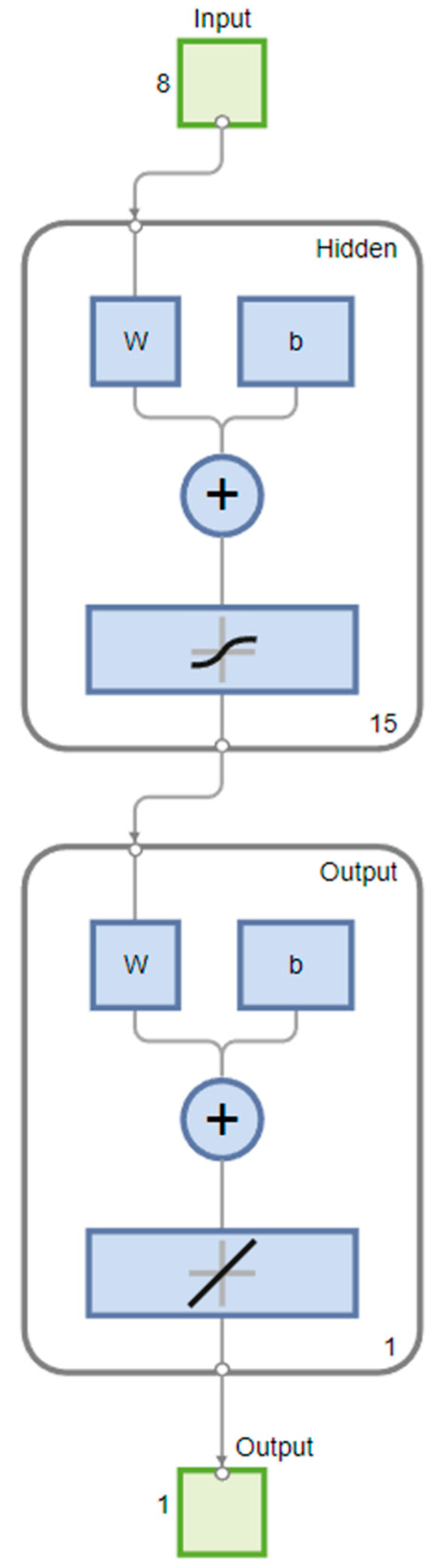
A neural network with a single hidden layer was constructed, varying the neurons from 2 to 20. The selection of this particular neuron count was the result of an iterative testing process. Various neuron configurations were evaluated to pinpoint the most effective number that strikes an optimal balance between the complexity of the model and its predictive performance. It evaluated three learning algorithms: Levenberg-Marquardt (L-M), Bayesian Regularization (BR), and Scaled Conjugate Gradient (SCG), chosen for their effectiveness. The L-M algorithm, though swift, is memory-intensive. Training ceases when validation errors stop decreasing, signaling overfitting. BR, albeit slower, tends to generalize better, particularly for complex datasets, halting training as it adjusts for overfitting. SCG, a more memory-efficient method, also stops when validation error reduction stalls. The dataset consisted of 225 observations. The dataset split was comprised of 75% for training, with the remaining 30% equally divided between validation and testing.

2.4. Modeling Methodology and Quality Indicators

The set of variables used included several energy metrics: Electricity prices by type of user, Energy productivity, Final energy consumption, Gross domestic product at market prices, Recycling rate of municipal waste, Domestic material consumption per capita, Environmental tax revenues, and Share of energy from renewable sources.

The initial phase of the study was dedicated to examining the interrelationships between variables through correlation analysis. This step is crucial as interdependencies among input variables can introduce ambiguity in the model’s learning phase. Typically, Pearson’s correlation analysis is employed to detect and mitigate multicollinearity by discarding one or more interdependent variables [38].

After analyzing the correlation and determining the input data for modeling energy recovery from MSW, the modeling phase began using three machine learning methods such as ElasticNet, Decision Trees, and Neural Networks. The methodology for the development of this research is shown in the flowchart below (Figure 1).

The quality of the models was evaluated based on specific metrics listed in

Table 3. Quality indicators used to evaluate the received models.

Quality Indicator	Formula	Meaning of Symbols
Regression value (R)	$\mathrm{R}\left({\mathrm{y}}^{\prime },{\mathrm{y}}^{\mathrm{*}}\right)=\frac{\mathrm{c}\mathrm{o}\mathrm{v}\left({\mathrm{y}}^{\prime },{\mathrm{y}}^{\mathrm{*}}\right)}{{\mathsf{\sigma }}_{{\mathrm{y}}^{\prime }}{\mathsf{\sigma }}_{{\mathrm{y}}^{\mathrm{*}}}}, \mathrm{R}\mathsf{ϵ}<0,1>$	σy′—standard deviation of reference values of the energy recovery, σy*—standard deviation of predicted values the energy recovery, yi is the actual value of the energy recovery, and ${\widehat{\mathrm{y}}}_{\mathrm{i}}$ denotes the value of the energy recovery for the i-th observation obtained from the model
Mean Squared Error (MSE)	$\mathrm{M}\mathrm{S}\mathrm{E}=\frac{1}{\mathrm{n}}{\displaystyle \sum _{\mathrm{n}=1}^{\mathrm{n}}}{\left({\widehat{\mathrm{y}}}_{\mathrm{i}}-{\mathrm{y}}_{\mathrm{i}}\right)}^2$
Root Mean Square Error (RMSE)	$\mathrm{R}\mathrm{M}\mathrm{S}\mathrm{E}=\sqrt{\frac{{\sum }_{i=1}^n{\left(y_i-{\widehat{y}}_i\right)}^2}{n}}$
Relative Importance of Errors (RIE)	$\mathrm{R}\mathrm{I}\mathrm{E}=\frac{‖y^{\prime }-y‖}{‖y‖}$
Mean Absolute Error (MAE)	$\mathrm{M}\mathrm{A}\mathrm{E}=\frac{1}{N}{\displaystyle \sum _{i=1}^N}\left(\left|y_i-{\widehat{y}}_i\right|\right)$

. The selection of quality indicators such as Regression Value (R), Mean Squared Error (MSE), Root Mean Squared Error (RMSE), Relative Importance of Errors (RIE), and Mean Absolute Error (MAE) is grounded in their robustness for evaluating predictive models. The Regression Value (R) assesses the strength and direction of the linear relationship between observed and predicted values. MSE and RMSE are crucial for determining the average power of prediction errors, with RMSE giving more weight to larger errors due to the squaring process. RIE offers a normalized comparison of errors, providing insight into the relative magnitude of predictive inaccuracies. Lastly, MAE provides an average of the absolute errors, which is especially useful for understanding the practical significance of the prediction errors in the context of energy recovery. Together, these indicators deliver a comprehensive understanding of model performance, balancing both the magnitude of errors and the consistency of the model’s predictive ability.

3. Results

Pearson’s correlation analysis was conducted to discern interdependencies among the input energy variables, with findings detailed in

Table 4. Correlation analysis results.

Variable	EPTU	EP	FEC	GDPMP	RRMW	DMC	ETR	SERS
EPTU	1.000000	0.749484	0.490864	0.443991	0.502364	−0.101240	0.064623	0.005785
EP	0.749484	1.000000	0.312311	0.716978	0.505365	−0.025537	−0.152443	0.048732
FEC	0.490864	0.312311	1.000000	0.132517	0.453852	−0.241893	0.161477	−0.209181
GDPMP	0.443991	0.716978	0.132517	1.000000	0.546917	0.248230	−0.155644	−0.157976
RRMW	0.502364	0.505365	0.453852	0.546917	1.000000	−0.003523	−0.196494	0.044154
DMC	−0.101240	−0.025537	−0.241893	0.248230	−0.003523	1.000000	−0.256747	0.478000
ETR	0.064623	−0.152443	0.161477	−0.155644	−0.196494	−0.256747	1.000000	−0.314553
SERS	0.005785	0.048732	−0.209181	−0.157976	0.044154	0.478000	−0.314553	1.000000

. No variable was highly correlated, so all parameters were included in further analyses.

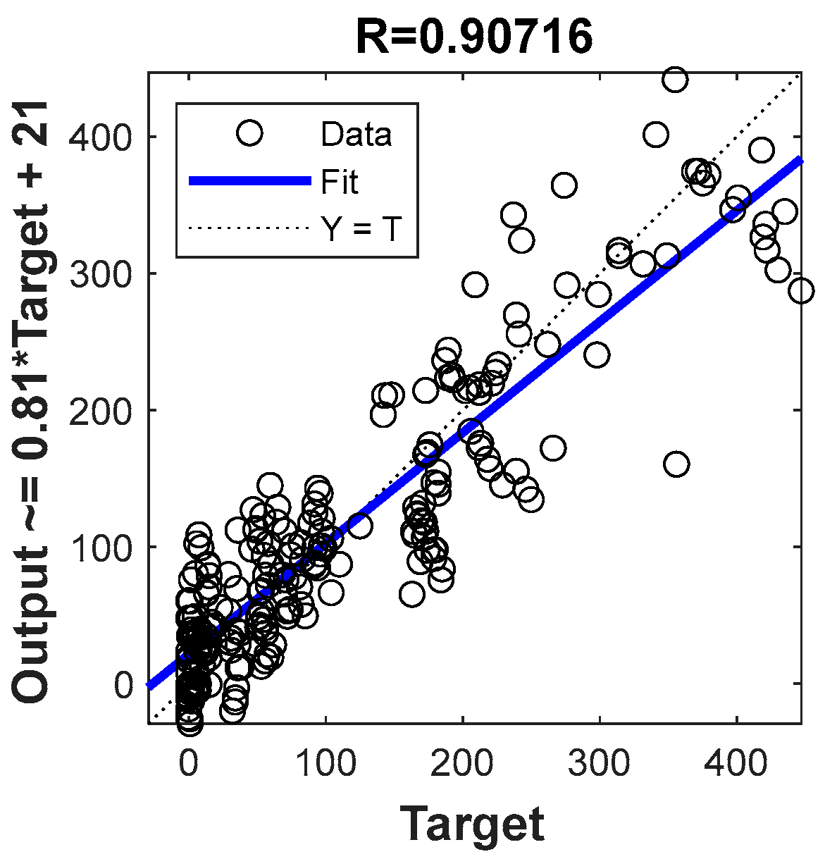
The first modeling method analyzed was ElasticNet, for which the best model was obtained with alpha set to 1 and lambda set to a very low value of 0.0001.

Table 5. Results of ElasticNet model quality indicators.

Quality Indicators	ElasticNet Model
R (all data)	0.90716
MSE	2372.8
RMSE	48.7114
RIE	0.3012
MAE	36.97

provides an exhaustive breakdown of all the key metrics. By setting alpha to 1, the strategy shifted toward the use of a lasso regression, emphasizing the importance of selecting significant features. The choice of a low lambda value, 0.0001, indicated a slight regularization effect to preserve the flexibility of the model. The performance of the model was remarkable, with a Mean Squared Error of 2372.8, demonstrating its ability to fit the data set. The model’s prediction error spread was captured by a Root Mean Squared Error of 48.7114. In addition, the model’s prediction accuracy was highlighted by a Relative Importance of Errors of 0.3012. The Mean Absolute Error of 36.97 underscored the model’s consistent predictive ability. The regression analysis of the entire data set with the ElasticNet model is shown in Figure 2.

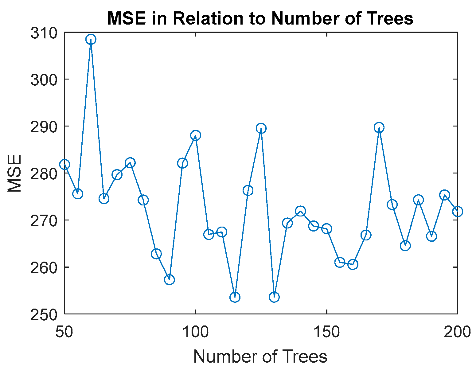
The second analyzed method for modeling the energy recovery is decision trees. The process involved varying the number of trees within a range from 50 to 200 trees, with a step of five trees. The best DT modeling results were obtained for 115 trees. The graph in Figure 3 shows the MSE for different numbers of trees in a DT model. The model’s consistent predictive ability was underscored by a MAE of 12.0148. Additionally, its performance was remarkable, with a MSE of 253.57, demonstrating its ability to fit the dataset. The prediction error spread was captured by a RMSE of 15.9239. Furthermore, the model’s prediction accuracy was highlighted by a RIE of 0.0984. These indicators are presented in

Table 6. Results of Decision Trees model quality indicators.

Quality Indicators	Decision Trees Model
R (all data)	0.9905
MSE	253.57
RMSE	15.9239
RIE	0.0984
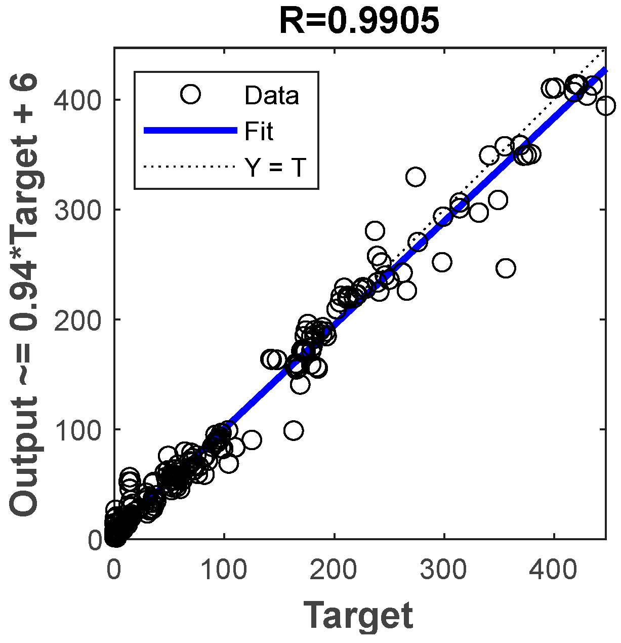
MAE	12.0148

. The regression analysis of the entire dataset with the DT model is shown in Figure 4.

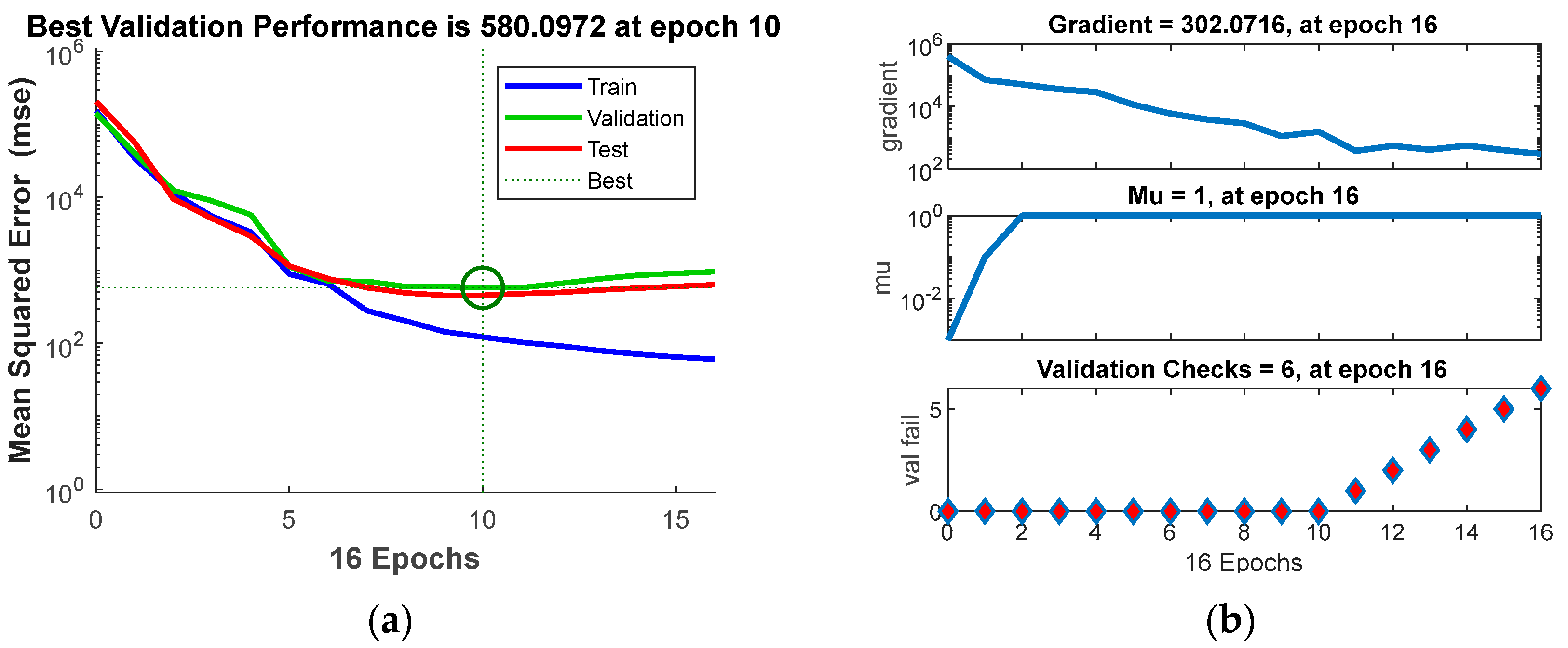
The previous method of analysis was neural networks. Optimal outcomes in neural network modelling were achieved using a hidden layer consisting of 15 neurons. The architecture of the neural network is illustrated in Figure 5. During the training phase, peak model efficiency was achieved at the 10th epoch, with a metric of 580.0972, as shown in Figure 6a.

Table 7. Summary of neural network training metrics.

Training Progress	The Best Neural Network Model
Training algorithm	Levenberg-Marquardt
Epoch	16
Performance	61
Best validation performance	5,800,972 at epoch 10
Gradient	302

summarizes the training progress metrics for the best neural network model, including the algorithm used, number of epochs, performance, best validation performance, and gradient values.

To prevent the model from overfitting, a scenario where it performs well on training data but poorly on new data, the training process was meticulously observed. A halt in training was initiated upon observing six successive rises in the error during validation, or if there was no improvement in error rates. This method, often referred to as “early stopping”, serves to preempt overfitting by ceasing training once there is a decline in the model’s validation performance. Figure 6b illustrates the progression of the network’s training process. 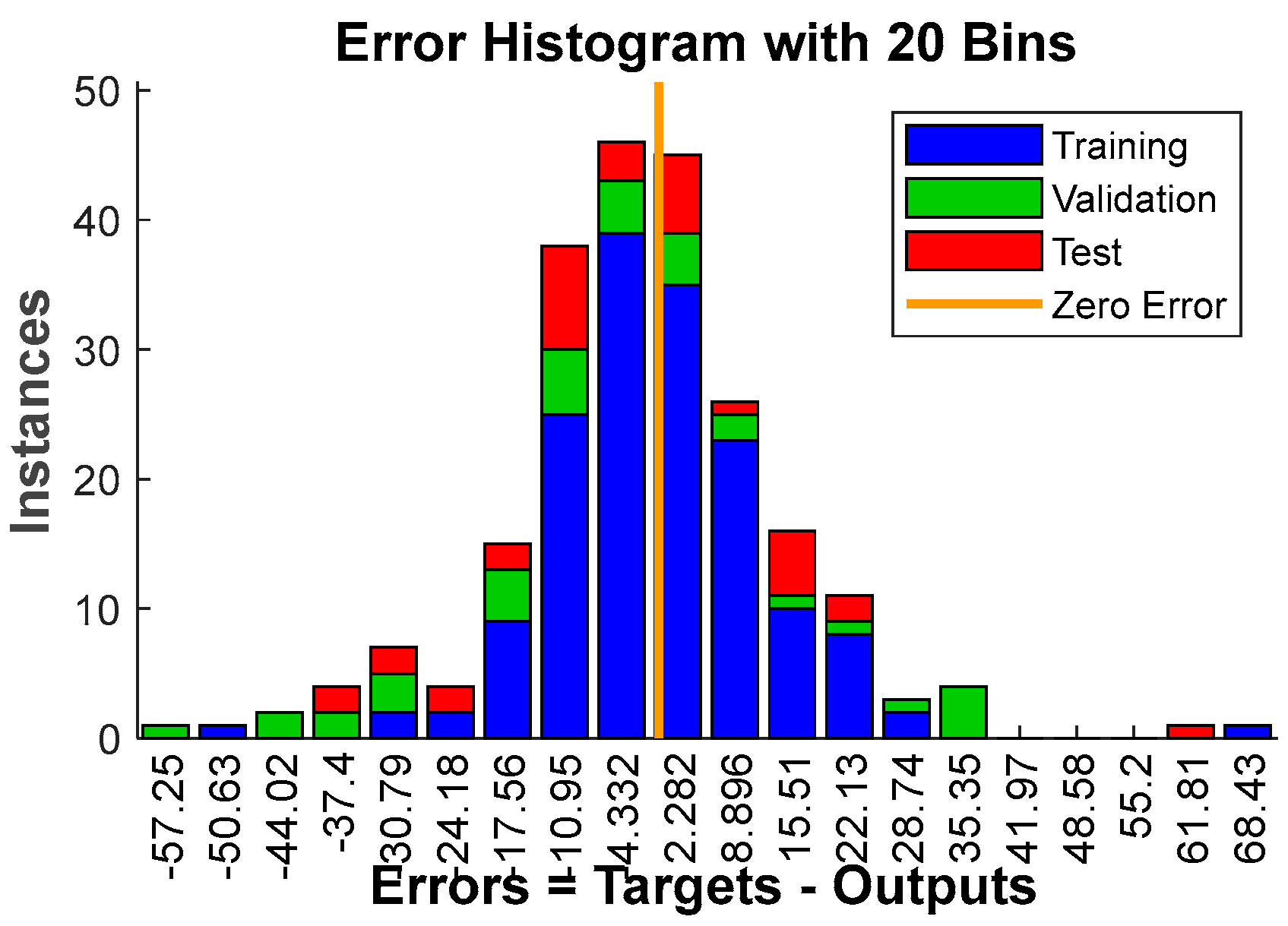Figure 7 shows an error histogram representing the distribution of errors between predicted results and actual targets in the process of training the best neural network model. The errors were divided into 20 ranges, indicating the frequency of errors in specific ranges. Most of the errors cluster around the zero-error line, indicative of a high number of predictions being close to the actual values. The shape of the distribution bears resemblance to a Gaussian curve, characterized by its symmetry around the mean error. This resemblance generally suggests that the errors are predominantly random and the model is not systematically overestimating or underestimating the targets.

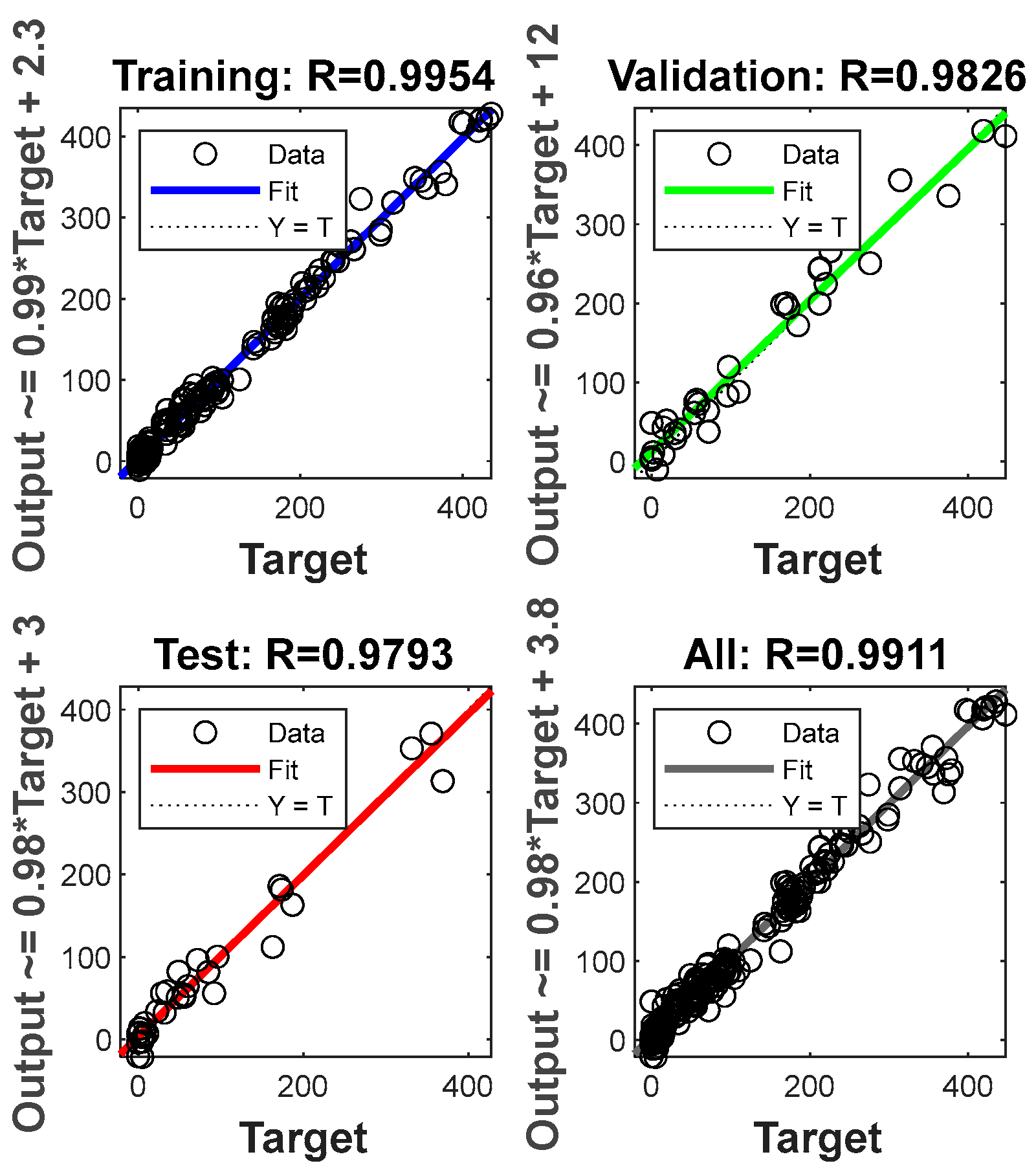
Figure 8 shows four scatter plots, each representing a different data set in the context of training a neural network model: training, validation, testing, and all data. Each scatterplot shows the relationship between predicted results (y-axis) and actual target values (x-axis), with a best-fit line indicating the model’s predictive performance. The dotted line Y = T represents the ideal scenario where the predicted output equals the target value. The closer the data points and the fit line are to this dotted line, the better the model’s predictions. The fact that the fit lines in each plot are close to the Y = T line indicates good model performance across all datasets.

The results of the comparison of the analyzed models are presented in

Table 8. Comparison of the analyzed models.

Quality Indicators	ElasticNet Model	Decision Trees Model	Neural Network Model
R (all data)	0.90716	0.9905	0.9911
MSE	2372.8	253.57	242.09
RMSE	48.7114	15.9239	15.5593
RIE	0.3012	0.0984	0.0962
MAE	36.97	12.0148	11.1631

. The quality of each model was compared using indicators such as R, MSE, RMSE, RIE and MAE. The ElasticNet model shows a lower R-squared value of 0.90716, suggesting it explains less variance in the data compared to the other two models, which both exhibit R-squared values closer to 1, indicating a very high degree of variance explanation. The MSE and RMSE for the ElasticNet model are substantially higher than those for the Decision Trees and Neural Networks, implying larger average and root-mean-squared prediction errors. In terms of the RIE, ElasticNet has the highest value, and Decision Trees the lowest, indicating that Decision Trees have the least relative error. Finally, the MAE is significantly higher for ElasticNet, somewhat lower for Decision Trees, and the lowest for Neural Networks, suggesting that the Neural Network model has the best average prediction accuracy among the three. In conclusion, while all models show competency in predictions, the Neural Network model outperforms the other two in terms of these quality indicators, with Decision Trees following and ElasticNet lagging behind, particularly in the error metrics.

4. Discussion

Three machine learning methods were used in the research presented: Elastic Net, Decision Trees, and Neural Network to model energy recovery from waste. The input data used were indicators related to different aspects of energy management, economics, and environmental protection: Electricity Prices by Type of User, Energy Productivity, Final Energy Consumption, Gross Domestic Product at Market Prices, Recycling Rate of Municipal Waste, Household Material Consumption per Capita, Environmental Tax Revenues, and Share of Energy from Renewable Sources. These data are used to forecast energy recovery because, taken together, they provide a comprehensive picture of both energy demand and supply, the effectiveness of its use, and the impact of environmental and economic policies on the energy sector. Analyzing these indicators provides a better understanding of how different factors affect the opportunities for energy recovery and identifies the trends that may affect future energy recovery needs and opportunities. Such a comprehensive approach is necessary to produce accurate and useful forecasts in a dynamically changing energy environment.

The research conducted indicates that the ANN model is more effective and accurate in predicting energy recovery from waste compared to the Elastic Net and Decision Trees methods. The calculation and analysis of the quality indicators of the machine learning models, such as R, MSE, RMSE, RIE, and MAE, allowed them to be evaluated in terms of accuracy, stability, and ability to generalize. High R values indicate a strong correlation between predictions and actual values, while high MSE and MAE values indicate less accurate predictions. The neural network model obtained the lowest MSE (242.09) and MAE (11.1631) and the highest R value (0.9911); it managed better with the input data. Decision trees, despite being a simpler model, also showed high efficiency: R = 0.9905, MSE = 253.57, and MAE = 12.0148, suggesting that the data structure fits well with regression-based models. ElasticNet, being a linear method, does not cope with the dependencies of the input data, which is manifested by higher errors (MSE = 2372.8; MAE = 36.97). When building ANN models, the choice of the number of layers, neurons, and activation functions offers much greater flexibility in adapting the model, making it a preferred choice for building models. The disadvantage of ANN models is the difficulty in interpreting the results obtained compared to ElasticNet and Decision Trees.

There are few models for forecasting energy recovery from waste based on economic, environmental or social indicators. Adamovic et al. (2018) developed a General Regression Neural Network model to forecast the annual production of primary energy from fixed municipal waste in European countries [39]. As input data they used the following: Human development index, Gross domestic product, Domestic material consumption, Urban population share, MSW recycling rate, MSW generated, Energy taxes, Share of renewable energy in gross final energy consumption, Energy productivity, Number of main electric retailers per million inhabitants, Final energy consumption, Electricity prices by medium-size industry, and Electricity prices by medium-size households. The model was characterized by the determination factor R² = 0.995 and the mean absolute percentage error MAPE = 7.757% [39]. Elshabour et al. (2021) developed an artificial neural network model to predict the amount of waste in Poland [40]. As input data, the following were used: Population, Income per capita, Employment to population ratio, Number of enterprises registered in the region per 10,000 inhabitants, and Number of enterprises by type of business activity. The model yielded R = 0.98 [40].

Comparative experiments are an important element in assessing the effectiveness of machine learning models. Much of the current research is based on a single machine learning model without considering other machine learning models [8,41]. It is important to conduct tests on different machine learning models, as each of them is characterized by unique advantages and disadvantages. Different models analyze data in their own way, which can lead to different results in terms of accuracy, efficiency, and usability for certain types of data. In the future, it will be crucial to create solid reference points and detailed descriptions of machine learning models, which will allow continuing research based on previous achievements as well as accelerate progress in the development of machine learning models and their application.

The studies presented show that machine learning models can predict energy recovery from waste. The modeling and prediction of energy recovery from waste using machine learning techniques and economic and environmental indicators can help to make investment decisions on potential sources and recovery technologies, optimize processes, and assess the economic and environmental impact of energy recovery projects. The use of these indicators allows for a more integrated and holistic approach to energy and waste management, which is crucial for promoting sustainable development.

5. Conclusions

This goal of this paper was to evaluate the most effective machine learning technique for predicting energy recovery from waste. It uniquely compares three methods: ElasticNet, Decision Trees, and Neural Networks, considering quality indicators such as R, MSE, RMSE, RIE, and MAE. ElasticNet had an R-value of 0.90716, but it also showed higher error metrics, such as an MSE of 2372.8, compared to Decision Trees and Neural Networks. Decision Trees had a lower MSE of 253.57 and an R-value of 0.9905, indicating better performance than ElasticNet. Neural Networks, with an R-value of 0.9911 and the lowest MSE of 242.09 along with the lowest MAE of 11.1631, slightly outperformed Decision Trees, suggesting it was the most accurate model among the three. The use of ‘early stopping’ to avoid overfitting and the Gaussian-like distribution of errors in the neural network error histogram suggest robust training methodologies were employed.

The comparison between ElasticNet, Decision Trees, and Neural Networks demonstrates that while all three methodologies offer valuable insights into energy recovery processes, Neural Networks exhibit a superior ability to handle the complex, non-linear relationships inherent in waste-to-energy data. This finding underscores the importance of adopting advanced computational techniques to enhance the predictive modeling of energy recovery systems.

This research opens the way for further studies to explore other machine learning algorithms, incorporate more diverse datasets, and extend the analysis to other regions and waste types. Investigating the economic and environmental impacts of implementing waste-to-energy solutions at scale can also provide valuable insights for sustainable development.