Clutter Map Constant False Alarm Rate Mixed with the Gabor Transform for Target Detection via Monte Carlo Simulation

Abstract

Radar detection is a technology frequently used to detect objects and measure the range, angle, or velocity of those objects. Several studies have been performed to improve the accuracy and performance of detection methods, but they encountered a strong challenge, which was the minimization of false alarms and the distinguishing of real targets from false alarms, especially in nonhomogeneous environments. We propose a new detection method that uses time-frequency analysis tools to improve detection performance and maintain a low constant false alarm rate. Different from existing works, this paper combines the clutter map constant false alarm rate technique with the Gabor transform for accurate target detection in cluttered environments. We suggest the combination of a CFAR detector with a time-frequency method that enables us to tackle challenging scenarios involving near targets. The proposed method allows for locating the exact position of the target by reducing the impact of clutter and maintaining a low rate of false alarms, while the Gabor transform facilitates the extraction of pertinent target characteristics and improves differentiation from clutter. Through experiments and simulations in different scenarios and clutter models, we demonstrate that the method is efficient in measurements and performs well in cluttered environments. This research has a major impact on signal processing and significantly improves target detection in cluttered environments, allowing this method to be deeply developed and implemented.

1. Introduction

Target detection is a crucial direction for radar research. Traditional target detection methods are usually based on constant false alarm rate (CFAR) detectors [1]. Nowadays, target detection methods have been developed using various advanced techniques, including signal processing techniques, optimization techniques, and machine learning techniques [2]. In modern radar systems, constant false alarm rate (CFAR) detection plays a crucial role in automatic detection [3]. However, nonstationary and nonuniform complex clutter can have an impact on the performance of the CFAR algorithms [4]. The ability to accurately identify targets in cluttered environments is crucial for effective decision making and situational awareness. However, clutter, which can be unwanted signals generated by stationary and nontarget objects, constitutes a significant challenge to target detection algorithms. Traditional detection methods often suffer from high false alarm rates or limited target discrimination capabilities, leading to degraded performance. Based on the power estimation method, CFAR detection can be split into two groups: those that use spatial processing and those that use temporal processing [5,6].

The clutter map constant false alarm rate (CMAP-CFAR) is a signal processing technique used to detect targets in cluttered environments. It is a type of CFAR algorithm that adjusts the threshold for detecting targets based on the level of clutter in the surrounding environment. Specifically, the detector output of each range-resolution cell is averaged over multiple scans to estimate the background level. Nitzberg [7] developed the CMAP-CFAR processor using digital filtering to update the background power estimate corresponding to each map cell in every scan [8]. There have been studies on CMAP-CFAR detection systems that explore various background distributions [9,10,11,12]. The main advantage of using a CMAP-CFAR algorithm is that it can help reduce the number of false alarms generated with the radar system. This is especially important in scenarios where the radar is operating in a cluttered environment, such as in a city or near a body of water. To enhance the efficiency of the CMAP-CFAR device, it could be combined with another technique to increase reliability and interest.

The Gabor transform is a useful technique for analyzing signals with both time-varying and frequency-varying characteristics. In radar signal processing, the Gabor transform can be used for detecting targets in cluttered environments. The clutter in radar signals can arise from various sources, such as the ground, sea, and buildings. These clutter signals can interfere with the detection of targets, making it difficult to detect them. The main aims of this study are to look into the pros and cons of current methods for finding targets in crowded areas, come up with a new method that combines the Gabor transform and the CMAP-CFAR algorithm, and then compare the existing method’s effectiveness with that of the proposed method to see how well it works and what changes could be made to make it better. All of these efforts aim to distinguish and differentiate target signals from clutter signals.

Several studies have been conducted on CFAR detection techniques to identify the most efficient technique. The authors of [3] proposed a study on a novel clutter map constant false alarm rate detector based on the power transform that utilizes the power transform for enhanced efficiency compared to traditional methods. After that, ref. [13] suggested a method, FPGA implementation of the efficient CFAR algorithm for radar systems, that focuses on hardware implementation and optimizing the algorithm’s speed and performance. Later, ref. [4] suggested a CFAR detection algorithm for cognitive radar that is based on clutter knowledge and includes cognitive elements that make it more flexible in cluttered environments. Another method was developed in [14], which is an improved constant false alarm rate detector based on multiframe integration for fluctuating target detection in heavy-tailed clutter. This method improves the robustness of fluctuating target detection in heavy-tailed clutter. In [15], they suggested the use of a multibeam seafloor constant false alarm detection method based on weighted element averaging, which is specifically tailored for seafloor applications, improving accuracy in underwater scenarios. Despite these efforts to propose new techniques, achieving satisfactory detection performance has proven to be challenging and complex to implement.

2. Mathematical Modeling and Analysis of the Proposed Detector Algorithm

2.1. Clutter Map CFAR Detector

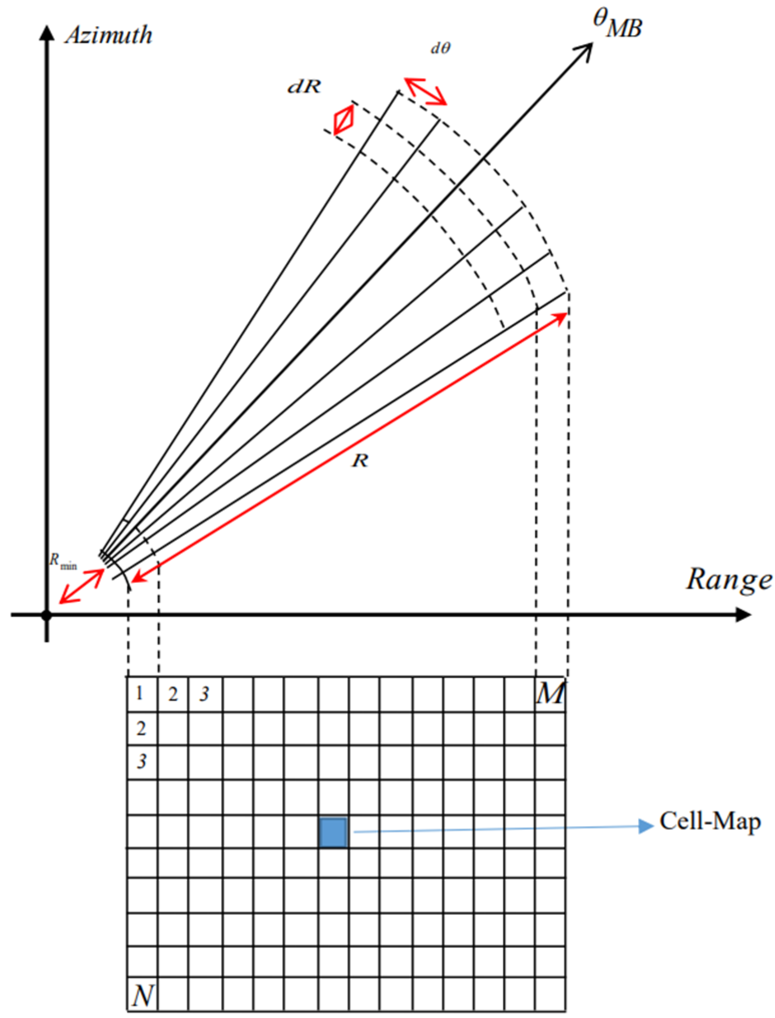
2.1.1. Description of the CMAP-CFAR Process

The CMAP-CFAR detector is a system using a first-order recursive filter to update the clutter power estimate. This detector uses a sliding window estimator that takes the average over m scans. Each resolution cell’s exponential smoothing updates the clutter power estimate at each scan of the radar space (see Figure 1).

In this technique, we use only the latest estimate instead of data from m previous scans. At each output of the kth cell of the Nth scan, the factor α is equal to q(k), where α is the filter’s coefficient gain used to ensure system stability (0 < α < 1) and is added to the previous estimate of clutter power y(n) weighted by the factor (1 − α) to obtain the new estimate.

Figure 2 represents the block diagram of our proposed detector where the threshold Th is calculated in a way to ensure a constant false alarm probability. By comparing the test cell q(k) with the weighted threshold, it is ultimately determined whether the target is present [16]. The background estimate is formed from the previous scans and for mth scan; the output of the recursive filter is given by the following equation:

$${\mathrm{y}}_{\mathrm{m}}\left(\mathrm{k}\right)=(1-\mathsf{\alpha })\times {\mathrm{y}}_{\mathrm{m}-1}\left(\mathrm{k}\right)+\mathsf{\alpha }\times {\mathrm{q}}_{\mathrm{m}}\left(\mathrm{k}\right)$$

(1)

where q_t is the output of the tth resolution cell and α is the filter’s coefficient gain. We can generalize Equation (1) recursively and obtain a more compact form, as shown below:

$${\mathrm{y}}_{\mathrm{m}}\left(\mathrm{k}\right)={\sum }_{\mathrm{i}=0}^{\mathrm{m}}\mathsf{\alpha }(1-\mathsf{\alpha }{)}^{\mathrm{i}}{\mathrm{q}}_{\mathrm{m}-\mathrm{i}}(\mathrm{k})$$

(2)

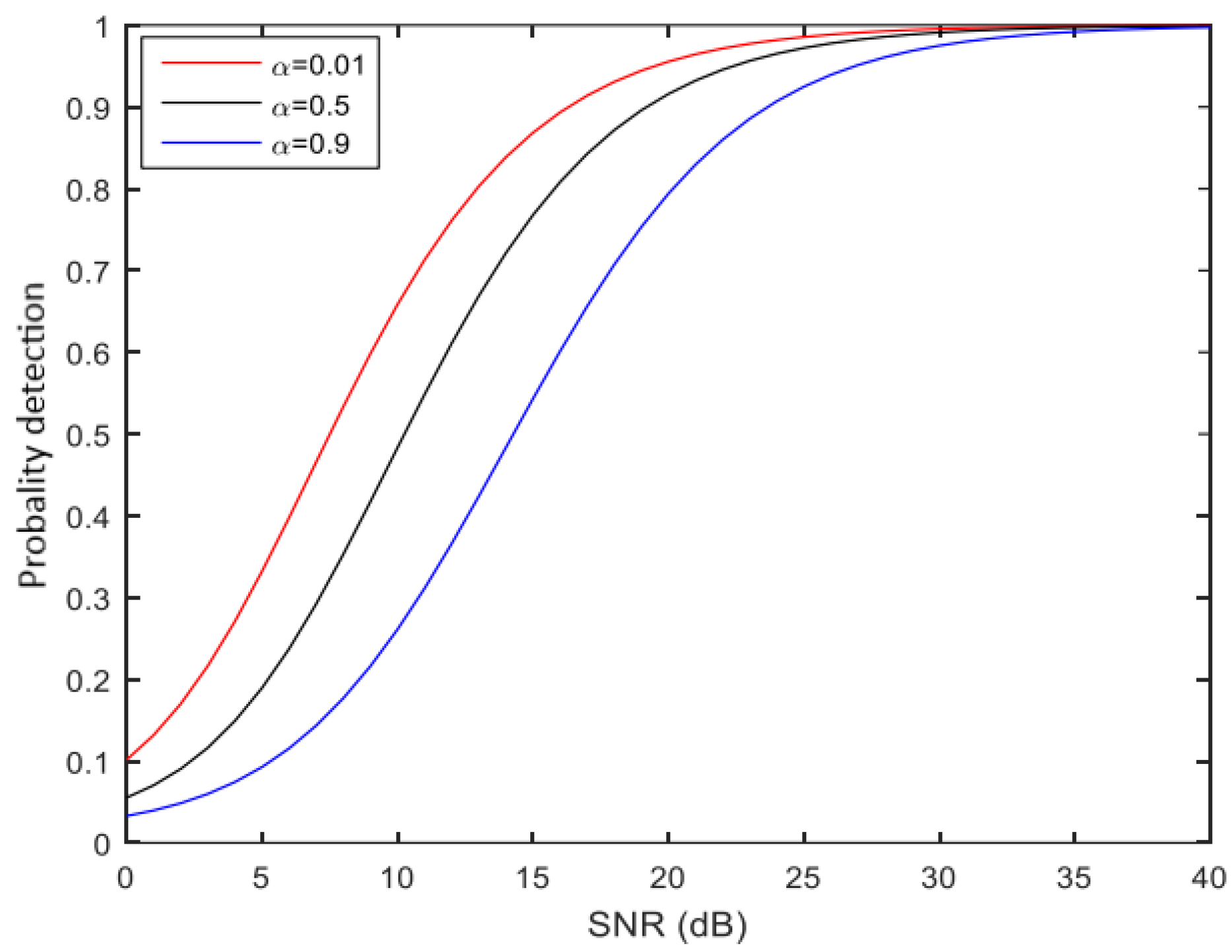
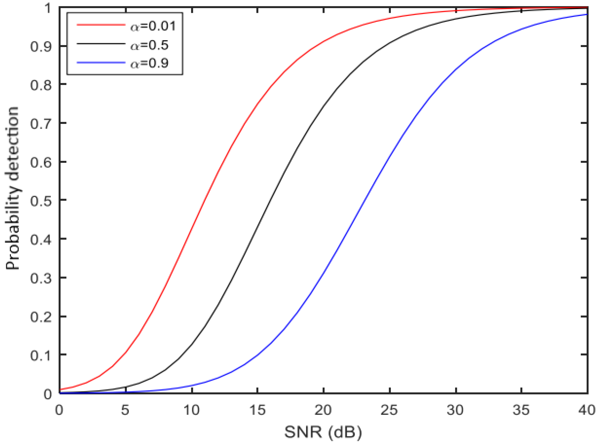
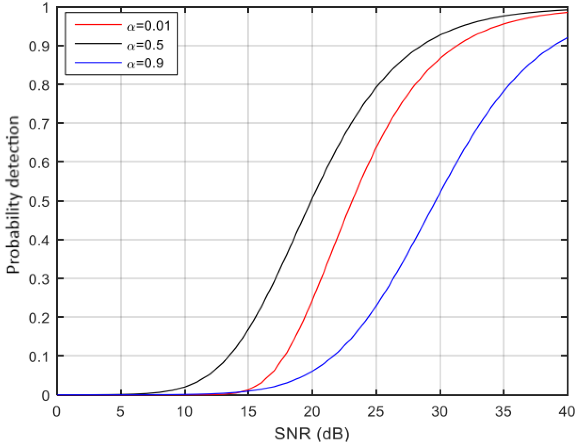
2.1.2. Probability of Detection

Reference [17] provides the conditional density functions for determining whether the target is present (alternative hypothesis H₁: presence of useful signal and clutter) or not (null hypothesis H₀: presence of clutter only). The probability densities corresponding to the presence and absence of the target at the detector output are given, respectively, by the following:

$$\mathrm{P}\mathrm{r}(\mathrm{q}\mid {\mathrm{H}}_0)=\left\{\begin{array}{c}\mathrm{P}\mathrm{r}(\mathrm{q}\mid {\mathrm{H}}_0)=\frac{{\mathrm{q}}^{\mathrm{P}-1}}{(\mathrm{p}-1)!}\mathrm{e}\mathrm{x}\mathrm{p}(-\mathrm{q})\\ \mathrm{P}\mathrm{r}(\mathrm{q}\mid {\mathrm{H}}_1)=\frac{{\mathrm{q}}^{\mathrm{p}-1}}{(\mathrm{p}-1)!(1+\mathrm{S}\mathrm{N}\mathrm{R}{)}^{\mathrm{p}}}\mathrm{e}\mathrm{x}\mathrm{p}(-\frac{\mathrm{q}}{1+\mathrm{S}\mathrm{N}\mathrm{R}})\end{array}\right.$$

(3)

where Pr(q|H₀) is the probability of false alarm (Pfa) and Pr(q|H₁) is the probability of detection (Pd).

Therefore, the probability of detection, given a fixed false alarm rate, is obtained by the following formula [14]:

$${\mathrm{P}}_{\mathrm{D}}={\int }_0^{\mathrm{\infty }}\mathrm{P}\mathrm{r}(\mathrm{y}){\int }_{\mathrm{T}\mathrm{h}}^{\mathrm{\infty }}\mathrm{P}\mathrm{r}(\mathrm{q}/{\mathrm{H}}_1)\mathrm{d}\mathrm{q}\mathrm{d}\mathrm{y}$$

(4)

Substituting (3) (case of hypothesis 1) into (4), we obtain the expression for the detection probability:

$$P_D={\sum }_{\mathrm{k}=0}^{\mathrm{n}-1}{\prod }_{\mathrm{n}=0}^{\mathrm{m}}(\begin{array}{c}\mathrm{n}+\mathrm{k}-1\\ \mathrm{k}\end{array}){(\mathrm{T}\mathrm{h}\frac{\mathsf{\alpha }\times (1-\mathsf{\alpha }{)}^{\mathrm{n}}}{1+\mathrm{S}\mathrm{N}\mathrm{R}})}^{\mathrm{k}}{(1+\mathrm{T}\mathrm{h}\times \frac{\mathsf{\alpha }\times (1-\mathsf{\alpha }{)}^{\mathrm{n}}}{1+\mathrm{S}\mathrm{N}\mathrm{R}})}^{-(\mathrm{n}+\mathrm{k})}$$

(5)

2.1.3. Probability of a False Alarm

The false alarm probability is given by the following equation [14]:

$$\mathrm{P}\mathrm{f}\mathrm{a}=\mathrm{P}\mathrm{r}(\mathrm{y}){\int }_{\mathrm{T}\mathrm{h}}^{\mathrm{\infty }} \mathrm{P}\mathrm{r}\left(\mathrm{q}/{\mathrm{H}}_0\right)\mathrm{d}\mathrm{q}\mathrm{d}\mathrm{y}$$

(6)

The results are obtained when the SNR = 0. The following is a result [14]:

$$\mathrm{P}\mathrm{f}\mathrm{a}=\left(\frac{1}{1+\mathsf{\alpha }\times (1-\mathsf{\alpha }{)}^{\mathrm{n}}\times \mathrm{T}\mathrm{h}}\right)$$

(7)

2.1.4. Analysis of the CMAP-CFAR

In this section, we analyze the performance of the CMAP-CFAR detector for a single pulse. We will plot the detection probability performance curves as a function of the SNR for different values of Pfa and α. We assume that the target is the Swerling I type, embedded in Weibull clutter. A Monte Carlo simulation is performed for different values of Pfa and α. The threshold Th is calculated from Equation (7). Given the weighting coefficient α, we vary the probability of a false alarm.

Table 1. Threshold values Th as a function of Pfa for different α values.

α	Pfa	Th
0.01	10−2	4.6
	10−4	9.4
	10−6	143
0.5	10−2	9
	10−4	31.4
	10−6	76.6
0.9	10−2	25.6
	10−4	190
	10−6	854

below shows the values of Th for different values of Pfa and α.

The following figures (Figure 3, Figure 4 and Figure 5) show the simulation results of the probability of detection as a function of the signal-to-noise ratio (SNR) and the coefficient α for different false alarm probabilities.

We examined the effect of the α filter gain settings on the probability of detection and the false alarm probability. We observe that for a small α, the probability of detection is better than that for a large α, which is normal since α is very small (α tends to 0), and the system tends to have a fixed threshold. On the other hand, when α is large (α tends toward 1), the previous samples are omitted to arrive at an estimate of the threshold, hence decreasing the probability of detection. The CMAP-CFAR detector exploits the local intrinsic homogeneity of the radar environment, in which the radar space is divided into clutter map cells (see Figure 1) [18]. It is best used for small radar-equivalent areas or targets flying tangentially to the circle formed by the target–radar core [19].

2.2. Clutter Map Cfar Mixed with the Gabor Transform Algorithm

2.2.1. Analysis Tools and Investigation Techniques

Let us consider a metric radar with a pulse width equal to 6 microseconds. The CMAP-CFAR method was first used to detect and determine if there were targets in the scanned cell. After the CMAP-CFAR tool decides on the presence of a target, we use the Gabor transform to verify whether there are several targets inside that cell. The OS-CFAR detector provides the final decision about the number of targets detected. This process can be seen in the following Figure 6, that represent the block diagram of the The joint use of a CFAR detector and a time-frequency technique allows us to address difficult cases (near targets).

2.2.2. Detection with the Gabor Transform

The Gabor transform, which is a linear time-frequency analysis technique, has long been recognized as a very useful tool in signal stationarity over time. It uses a Gaussian window to create a time sample from which the spectrum of local signal values is calculated [19]. Any finite sequence X(k) that is periodized can be decomposed based on a shifted Gaussian distribution and amplitude modulation. The following equation defines its discrete Gabor expansion [18]:

$$X(k)={\sum }_{n=0}^{N-1} C_{mn}h(k-mN)e^{2j\pi \frac{kn}{N}}$$

(8)

where C_mn (m, n $\in \mathbb{Z}$) are the Gabor coefficients, m (m = 1 … M) and n (n = 1 … N) are the time and frequency samples, respectively, and k (k = 0 … NM−1) represents the samples of the finite sequence X(k). The coefficients of the Gaussian window chosen with the Gabor transform are calculated from the following equation:

$$h(n)=e^{-\frac{1}{2}{\left(\mathsf{\alpha }\frac{2n}{N_h}\right)}^2}$$

(9)

Hence, N_h is the width of window h, and α is proportional to the inverse of the standard deviation. The analysis window h, which is both well localized in time (if h is short) and in frequency (if h is long), must also be at finite energy, as shown in the following equation:

$${\sum }_{k=0}^{L-1} |h(n){|}^2⟨\infty$$

(10)

The Heisenberg inequality applied to a Gabor transform [20] constitutes a determining property when we want to treat the resolution in time and frequency jointly:

$$\mathsf{\Delta }T\times \mathsf{\Delta }F\ge \frac{1}{4\pi }$$

(11)

The coefficients {C_mn} are given by the following equation [19]:

$$C_{mn}={\sum }_{k=0}^{L-1} X(k)\gamma (k-mN)e^{-2j\pi \frac{kn}{N}}$$

(12)

where L = MN and j is the imaginary unit. M and N are the numbers of Gabor sampling points in time and frequency domains.

The synthesis window $\gamma (k)$ is a time window associated with the analysis window h(k) so that the orthogonality condition is verified [18]:

$${\sum }_{k=0}^{L-1} h_{-m,-n}(k)\gamma (k)={\delta }_m{\delta }_n$$

(13)

where δ_k is the discrete version of the delta function.

In order to choose the best parameters (N_h and α) for the proposed detector, we show the analysis window h and its corresponding synthesis window $\gamma$ with different values of N_h and α in the following figures (see Figure 7, Figure 8 and Figure 9):

Once the Gabor coefficients are calculated, again consider the squared modulus of the Gabor coefficients from Equation (12), and by projection on the time axis, as shown in Figure 10, we calculate the maximum instantaneous frequency of the frequency sample (n) for each temporal sample (m). Finally, we preserve these instantaneous powers (m) in an energy vector Y as follows:

Y(m) = MAX(|C_mn|²)

(14)

To better clarify the vector Y(m), Figure 10 presents the envelope detector based on the Gabor transform.

Finally, we obtain a spectrogram based on the Gabor transform, which represents an estimate of the signal’s power and its instantaneous frequency content [21].

2.3. Clutter Models

In order to show the performance of the proposed detector, three clutter models were considered for the simulation scenarios. For each scenario, a Monte Carlo simulation was carried out.

2.3.1. Model 1: Targets Drowned in a Cluttered Weibull Distribution

In this model, we introduce noise in the real parameters of our targets with a Weibull clutter distribution. The probability of the density function being a function of the parameters of scale a, shape b, and normalized amplitude $\nu$ > 0 is given by the following equation [14]:

$$p(\nu )={\left(\frac{\nu }{b}\right)}^{a-1}{e}^{-{\left(\frac{\nu }{b}\right)}^{\mathrm{a}}}$$

(15)

2.3.2. Model 2: Targets Embedded in Rayleigh Distribution Clutter

This model considers the same parameters as model 1, except that the shape parameter is equal to 1. The Rayleigh distribution with b and amplitude parameters normalized to ν > 0 is given by the following equation [22]:

$$p\left(v\right)=\frac{1}{b}{e}^{-\left(\frac{v}{b}\right)}$$

(16)

2.3.3. Model 3: Targets Drowned in Usual Clutter Distribution

In this case, a normal distribution with random variables of mean μ and standard deviation σ models the clutter distribution. The probability density function is given by the following equation [14]:

$$p(\nu )=\frac{1}{\sigma }{e}^{\frac{-{(\nu -\mu )}^2}{2{\sigma }^2}}$$

(17)

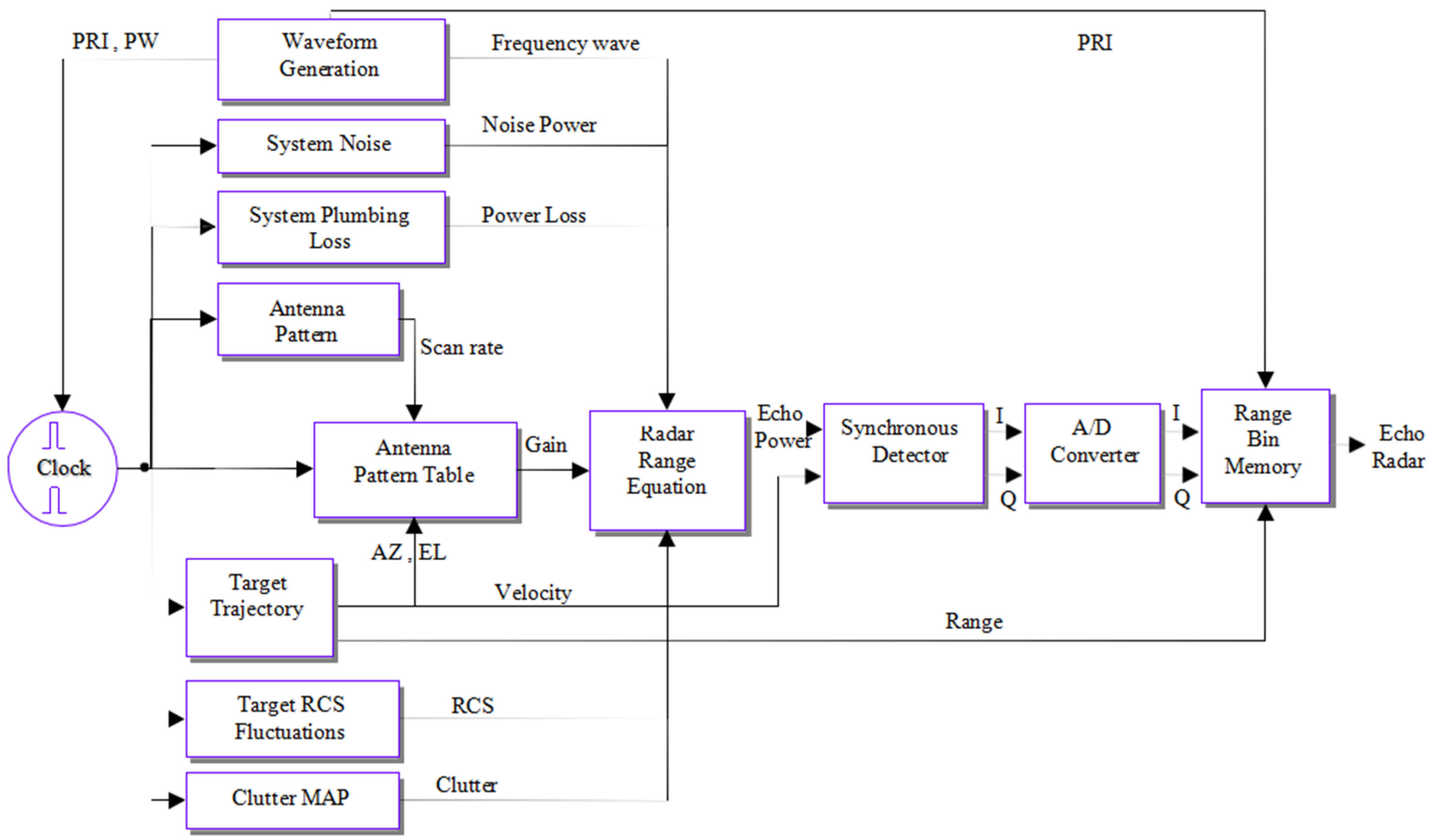
2.4. Radar Signal Simulation

The radar equation (Equation (18)) calculates the echo amplitude, including the radar parameters shown in

Table 2. Radar parameters.

Radar Parameters	Symbols	Values
RF frequency	f	900 MHz
IF frequency	If	30 MHz
Pulse repetition frequency	PRF	1 kHz
Peak transmit power	Pt	280 kWatts
Pulse width	τ	6 μs
Main beam gain	Gt	28.5 dB
−3 dB HPBW	HPBW	3.3°
Up spot angle elevation	El_up	12°
Scan rate	Fs	72°/s
Scan sector (min to max)	Scan_sec	25°
Receiver bandwidth	Bn	1 MHz
Doppler filter bank	Nf	32
Figure noise	Fn	2.5
IF amplitude gain	Aif	10 dB
Total radar loss	Loss	20 dB

and the target properties of each scenarios.

$${\mathrm{R}}_{\mathrm{m}\mathrm{a}\mathrm{x}}=\sqrt[4]{\frac{{\mathrm{P}}_{\mathrm{s}}{\mathrm{G}}^2{\mathsf{\lambda }}^2{\mathrm{A}}_{\mathrm{c}}\mathsf{\tau }}{{\mathrm{k}}_{\mathrm{B}}{\mathrm{T}}_0{\mathrm{F}}_{\mathrm{N}}{\left(4\mathsf{\pi }\right)}^3{\mathrm{L}}_{\mathrm{s}}}}$$

(18)

where P_r reflected power (in Watt), P_s: power emitted (in Watt), R_max: target–radar distance (in m), G: antenna gain, τ: Pulse width, k_B: Boltzmann constant (in J/K), T₀: absolute temperature (in °K), F_N: background noise from the receiver, L_s: radar system losses in transmission and reception, β: The bandwidth of the receiver, with $\mathsf{\beta }=\frac{1}{\mathsf{\tau }},$ and A_c: Apparent reflection surface of the radar antenna, with $A_c=\frac{G{\lambda }^2}{4\pi }$.

The radar receiver is modeled as shown in Figure 11 and is implemented using the set of real parameters of a search radar.

The radar echo X(m) is composed of a useful signal s(m) and an unwanted noise b(m). All the noises here are considered additive noises:

X(m) = s(m) + b(m)

(19)

The following figure (Figure 12) illustrates the probability density function of the signal X(m) and shows that the radar echo at the output of the proposed detector follows an exponential distribution [23].

We clearly see that the histogram of the radar echo X(m) (see Figure 12) is exponential in shape independently of the clutter model at the input of the proposed detector.

3. Simulation Results and Interpretation

Several simulations were conducted to analyze the impact of multiple targets on the range and azimuth resolution of radar echoes. During these simulations, each time we change the type of clutter as well as the parameters of each clutter for the two scenarios. In the first scenario, we simulated two radar targets in a resolution cell (dR, dθ) with only a variation in distance. The remaining target parameters were kept constant to demonstrate the range resolution of the proposed detector. In the second scenario, we examined how multiple targets affect radar resolution. In all the scenarios, we compared the performance of our proposed method with that of the normal order statistic constant false alarm rate (OS-CFAR) method. The OS-CFAR method, a reliable technique that Rohling [24] proposed, is appropriate for nonhomogeneous environments and is based on order statistics. This process involves ordering the cells of the reference window and selecting the content of the kth cell as an estimate of clutter power. To demonstrate the performance of the studied detector, we conducted several Monte Carlo simulations [25] for the different types of clutter in each scenario.

3.1. Scenario 1: The Effect of Distance

The choice of the parameters indicated in the following table is based on the studies of several researchers to bring our simulation closer to reality. In this scenario, we consider two targets with the parameters presented in

Table 3. Target properties in scenario 1.

Parameters	Symbols	Target 1	Target 2
Distance	R	88 km	80.5 km
Azimuth angle	θAZ	10°	10°
Speed	ʋ	333.3 m/s	333.3 m/s
Altitude	Alt	2200 m	2200 m
Hidden corner	ƞ	200°	200°
Radar cross-section	SER	1 m2	1 m2

below.

First, we simulated the two targets very close in distance (they are in the same resolution cell) and in the absence of clutter such that the OS-CFAR detector alone cannot distinguish them. In the second case, each target is simulated in a separate resolution cell. As shown in Figure 13, the target spot in red is shown on the panoramic display of our radar system (Plan Position Indicator PPI).

The number of reference cells (N_os) of the OS-CFAR detector is greater than 24, and the variable k is more significant than 3/4 of the number of N_os. These chosen parameters prove to result in better performance in terms of the probability of detection and guarantee a minimum number of false alarms. The OS-CFAR detector configuration parameters are grouped into

Table 4. Conventional OS-CFAR parameters.

Parameters	Values
Nos	24
k	24
NG	2

.

In Figure 14, we have the OS-CFAR detector and the target amplitude where it can be observed that there is one target amplitude that goes above the limit of the detector at around 84km, allowing the target to be detected. It goes along with the position of the target displayed by the PPI (Figure 13), showing the target at approximately the same position.

The detector based on the Gabor transform (proposed detector) is characterized by 64 samples on the time axis and 8 samples on the frequency axis. The analysis window h(n) is 32 cells in width, and the degree of oversampling q equals 1. The configuration parameters of the Gabor-based detector are grouped in

Table 5. Configuration parameters of the Gabor-based detector.

Parameters	Values
h(t)	Gaussian
Nh	32
M	64
N	8
q	1

.

Figure 15 shows the targets detected with the OS-CFAR method and those obtained using the proposed detector without clutter.

We observe in Figure 15b that the proposed detection method easily finds the position of the targets at M = 36 for the first target and at M = 43 for the second target. Compared to the conventional OS-CFAR detector, which detects a single target in the 84 km range (see Figure 15a) and the second target is missed. The proposed detector has been able to detect the two targets simulated here, while the OS-CFAR method detected a single target.

3.1.1. Simulation with Clutter Model 1

Figure 16 presents the simulation of two targets with clutter model 1 (targets drowned in a cluttered Weibull distribution). The clutter according to the first model is of the Weibull type; the shape parameter a and scale parameter b are chosen arbitrarily such that a = 25 and b = 0.9.

In Figure 16, we have the results obtained from the simulation using the OS-CFAR detection method (Figure 16a) and the proposed detection method (Figure 16b). We observe that in Figure 16b, the proposed detector finds the position of the two targets at M = 36 for the first one and at M = 43 for the second one. Compared to the conventional OS-CFAR detector, which detects a single target in the 84 km range (Figure 16a) and the second target is missed. The proposed detector has been able to detect the two targets simulated here, while the OS-CFAR method detected a single target.

We conducted another simulation, increasing the shape parameter a to 200 while keeping the scale parameter b at 0.9.

In Figure 17 we can observe in that (a) the target amplitude and false alarm rate are very high when it comes to the OSCFAR detector, while in (b) the proposed detector efficiently work on reducing the false alarm rate and is able to distinguish the target from the false alarm, the proposed detector is able to distinguish the target positions at M = 38 for the first target and at M = 43 for the second target (see Figure 17b). On the other hand, the conventional OS-CFAR detector detects multiple targets (Figure 17a), one of which is located at a range of 84 km, while the remaining targets are false alarms.

To further evaluate the efficiency of the proposed detector, we varied the shape parameter a within the range of 0 < a ≤ 200 and the scale parameter b below 0.5 (b < 0.5).

In Figure 18, we observe that the target amplitudes are lesser than in the previous simulation, but the proposed detector (Figure 18b) easily distinguish one target at M = 38 then hardly distinguish the second one at M = 39, while the OS-CFAR detector consider the actual targets and several false alarm as targets as displayed in Figure 18a. When the scale parameter is less than 0.5 and the shape parameter exceeds 200, the conventional OS-CFAR detector (see Figure 18a) fails to locate the targets and the proposed detector (see Figure 18b) hardly distinguishes the two targets. This test allows us to identify the limit in shape and scale when using our detector in the case of targets that are drowned in a cluttered Weibull distribution.

3.1.2. Simulation with Clutter Model 2

We present the simulation of two targets using clutter model 2 (targets embedded in Rayleigh distribution clutter). The shape parameter b of the Rayleigh distribution is confined to the interval [0,300] (Figure 19, Figure 20 and Figure 21).

We gradually increased the shape parameter b (b = 100, b = 200, and b = 300). In Figure 19b, Figure 20b and Figure 21b, we observe the ability of the proposed detector to successfully reduce the false alarms and clearly distinguish the two target positions, with the first target at M = 36 and the second target at M = 43. On the other hand, in Figure 19a, Figure 20a and Figure 21a, the conventional OS-CFAR detector detects multiple targets, one of which is located at a range of 84 km, while the remaining targets are false alarms. We clearly observe the differences between target amplitudes in the case of the conventional OS-CFAR detector and the target amplitudes in the case of our detector, which allow us to show the efficiency of the proposed method.

To assess the limits of the proposed detector in this case of clutter model 2, we increase the shape parameter b > 300. We set the shape parameter b at 600 (b = 600) and ran the simulation three times.

After the simulations, we observe that, in Figure 22b, the proposed detector shows the presence of two targets at M = 40 and M = 44, while the conventional OS-CFAR detector shows only one target, and the rest are false alarms. When we repeat the simulation with the same configuration (Figure 23 and Figure 24), the proposed detector once again detects the two targets but at different positions M = 36 and M = 45 for Figure 23b, then M = 39 and M = 43 for Figure 24b. The conventional OS-CFAR detector still distinguishes several targets where one is at M = 83 while the others are false alarms.

3.1.3. Simulation with Clutter Model 3

We performed a simulation of the two targets using clutter model 3 (targets drowned in cluttered normal distribution). The clutter follows a normal distribution with a standard deviation σ and a mean μ.

During the simulation using the clutter of model 3 with μ = 1 and σ = 1000, we observed the same limitations on detection performance in both models 1 and 2 (cases where the parameters have been increased) for the conventional detector, and our proposed detector has been able to distinguish the targets at M = 33 and M = 40. This situation can be seen in Figure 25.

We have summarized the key parameters of our simulations in the following

Table 6. Summary of the simulation of scenario No. 1.

Clutter Model	Clutter Parameters				Target Detected by OS-CFAR Alone		The Target Detected by the Proposed Detector			The Exact Position of the Targets
	a	b	σ	μ	Range (km)	Number of False Alarms	Target 1	Target 2	Number of False Alarms	Target Range1	Target Range2
Clutter-free					84	0	M = 36	M = 43	0	R = 80 km and M = 36	R = 80.5 km and M = 43
Weibull distribution	25	0.9			84	2	M = 36	M = 43	0
	200	0.9			84	7	M = 38	M = 43	0
	200	0.3			100	7	M = 38	M = 39	0
Rayleigh distribution		100			84	0	M = 36	M = 43	0	R = 80 km and M = 36	R = 80.5 km and M = 43
		200			84	5	M = 36	M = 43	0
		300			84	5	M = 36	M = 43	0
		600			84	5	M = 40	M = 44	?
		600			84	0	M = 36	M = 45	0
		600			84	7	M = 39	M = 43	0	R = 80 km and M = 36	R = 80.5 km and M = 43
Normal distribution			1000	1	?	?	M = 33	M = 40	?

“? means the number is undefined”.

in order to show the effect of the clutter on the distance resolution of radar targets. The results obtained are encouraging us to use our proposed method.

In this scenario, we have presented several Monte Carlo simulations for three different types of clutter models to demonstrate the performance of the proposed detector. In general, we observed that the proposed detector was able to reduce the false alarms and find the two targets used for the simulations, while the conventional detector (OS-CFAR) failed to distinguish the existing targets from the false alarms, serving as a benchmark for evaluating the efficiency of the proposed detectors.

3.2. Scenario 2: Effect on the Number of Targets

The second scenario consists of three targets that have the same parameters (

Table 7. Properties of the targets in scenario 2.

Scenario of Targets	Symbols	Target 1	Target 2	Target 3
Distance	R	80 km	80.4 km	80 km
Azimuth angle	θAZ	10°	10°	16°
Speed	v	333.33 m/s	333.33 m/s	333.33 m/s
Altitude	h	2200 m	2200 m	2200 m
Hidden corner	η	200°	200°	200°
Radar cross-section	RCS	1 m2	1 m2	1 m2

) except for the range and azimuth.

The Doppler frequencies of the three targets (C1, C2, and C3) are shown in Figure 26 to show the separation power of the proposed detector and the conventional detector.

We maintained the same OS-CFAR settings as in the previous scenario 1 for this simulation.

In Figure 27, we observe that the new detector visibly separates the three targets from the false alarm at time offsets M = 39, M = 46, and M = 54, but we still produce three false alarms close to each target. These three target positions will be considered as references for the rest of the simulations.

3.2.1. Simulation with Clutter Model 1

We simulated the three targets with clutter model 1 (targets drowned in a cluttered Weibull distribution), where the targets are drowned in the Weibull distribution with shape parameter a and scale parameter b chosen arbitrarily such that a = 25 and b = 0.9.

In Figure 28, we observe that the proposed detector successfully distinguishes the three targets used for the simulation at different positions (M = 41, M = 51, and M = 61).

We increased the shape parameter a to 250 (a = 250) and maintained the scale parameter b at 0.9 (b = 0.9) to simulate the three targets. We maintain the same value of the RCS for the simulations; the temporal and frequency values of the Gabor transform are M = 64 and N = 8 for the first simulation, then M = 64 and N = 32 for the second simulation.

After the simulations, we noticed a difference in the detected energy of the three targets (Figure 29) at M = 43, M= 52, and M = 62 compared to the previous simulations (Figure 28). There was a slight shift in the position of the targets in the reference positions after increasing the shape parameter a to a value greater than 200 (a = 250). In Figure 30, when we change the value of the frequency of the Gabor transform N from 8 to 32 we observe that our detector is able to detect only one target at M = 45, while the OS-CFAR detector distinguished several false alarms with high target amplitudes.

We decreased the shape parameter a to 25 (a = 25) and maintained the scale parameter b at 0.9 (b = 0.9) to simulate the three targets. We maintained the same value of the RCS for the simulation and decreased the temporal and frequency values of the Gabor transform to M = 32 and N = 16.

We observe that the proposed detector fails to distinguish all targets within the same range when we decrease the temporal and frequency values of the Gabor transform to M = 32 and N = 16, respectively. Only two targets were distinguished with the proposed detector at M = 23 and M = 28, as shown in Figure 31.

3.2.2. Simulation with Clutter Model 2

We realized the simulation of the three targets with clutter model 2 (targets embedded in Rayleigh distribution clutter) and a scale parameter b = 200, considering the temporal and frequency values of the Gabor transform to be M = 64 and N = 16, respectively.

In Figure 32, the simulation of the targets with clutter model 2 and a scale parameter b = 200 reveals that the proposed detector was able to detect only two targets, instead of all the three targets used for the simulation, at M = 48 and M = 58.

We maintained the scale parameter b = 200 but modified the temporal and frequency values of the Gabor transform to M = 128 and N = 8 for the first simulation then increased the scale parameter to b = 250 for the second simulation.

We observe in Figure 33 and Figure 34 that the proposed detector was able to distinguish the three targets at M = 81, M = 102, and M = 120 when we increased the temporal and frequency values of the Gabor transform to M = 128 and N = 8. The proposed detector successfully distinguishes the position of the targets while the OS-CFAR detector was able to just distinguish one target at M = 83 with low false alarms.

3.2.3. Simulation with Clutter Model 3

We performed a simulation of the three targets using clutter model 3 (targets drowned in cluttered normal distribution). The clutter follows a normal distribution with a standard deviation σ = 400, the temporal and frequency values of the Gabor transform are M = 128 and N = 8 for the first simulation then M = 256 and N = 2 for the second simulation.

We observe in Figure 35 that we encountered a limitation with the proposed detector when using clutter model 3 with a standard deviation σ equal to 400. In both figures, we see that the proposed detector is not able to clearly distinguish the three targets and has several false alarms, which is the same for the OS-CFAR detector. Despite increasing the temporal value of the Gabor transform to M = 256 and decreasing the frequency value to N = 2, we still face challenges, and the proposed detector is still not able to distinguish the three targets from all the false alarms obtained (Figure 36).

The simulation results for scenario No. 2 are summarized in

Table 8. Summary of the simulation of scenario No. 2.

Clutter Model	Clutter Parameters				Target Detected by the OS-CFAR Detector Alone			The Target Detected by the Proposed Detector
	a	b	σ	μ	Range (km)	Nfa	Nos	Target1	Target2	Target3	Nfa	M	N	q
Without clutter					82	1		M = 39	M = 46	M = 54	0	64	8	1
Weibull distribution	25	0.9			81	9		M = 41	M = 51	M = 61	0	64	8	1
	250	0.9			84	9		M = 43	M = 52	M = 62	0	64	8	1
	250	0.9			?	?		?	?	M = 45	?	64	32	1
	25	0.9			?	?		?	M = 23	M = 28	2	32	16	2
Rayleigh distribution		200			83	12	10	?	M = 48	M = 58	1	64	16	1
		200			83	11	10	M = 81	M = 102	M = 120	0	128	8	1
		250			81	12	10	M = 81	M = 102	M = 120	1	128	8	1
Normal distribution			400	10	?	?	10	?	?	?	?	128	8	1
			400	10	?	?	10	?	?	?	?	256	2	1

“? means the number is undefined”.

below. Knowing that Nfa represents the number of false alarms, at each detection limitation, for extreme clutter conditions, we adjusted the time and frequency parameters of the Gabor transform to enhance target detection. We therefore note that there is a possibility of detecting a target. On the other hand, for the N_os number of the OS-CFAR detector, we observed that reducing the N_os improved the ability of the proposed detector to distinguish targets.

We presented in each scenario several Monte Carlo simulations for the different types of clutter in order to show the performance of the proposed detector. The conventional detector (OS-CFAR) has not been able to clearly distinguish all the three targets used in the simulations; it could not separate existing targets from the clutter involved in the simulations, while the proposed detector has shown better performance by being able, in the cases of clutter free, clutter model 1, and clutter model 2, to distinguish the three targets used for the simulations. Additionally, we observed limitations of our detector in certain cases related to the clutter models. These cases occurred when we increased the frequency of the Gabor transform N from 8 to 32 for the Weibull distribution and when the time and frequency values of the Gabor transform were, respectively, M = 64 and N = 16 for the Rayleigh distribution, where target separation could not be improved. The same problem occurred when we had the standard deviation σ equal to 400. As anticipated, increasing the number of targets affects the efficiency of the proposed detection by decreasing the probability of detection and increasing the number of false alarms. The obtained results in the simulations helped to demonstrate the superior performance of the proposed detector compared to the OS-CFAR detector, even when the targets were very close in distance, azimuth, and speed.

To better illustrate the difference and progress between the proposed method of this work and other methods that have been developed previously, a table of method comparisons (

Table 9. Comparison with the state-of-the-art.

No.	Titles	Methods	Advantages	Limits	References
1	Clutter Map Constant False Alarm Rate Mixed with the Gabor Transform for Target Detection via Monte Carlo Simulation	detection method that uses time-frequency analysis tools via clutter map constant false alarm rate mixed with the Gabor transform for target detection.	• Reduce the impact of clutter and maintains a low rate of false alarms. • Significantly improves the detection probability and reduces the false alarm rate. • Facilitates the extraction of pertinent target characteristics and improves differentiation from clutter.	• Low efficiency when the number of targets is increase and when parameters linked to each clutter model are significantly increased or reduced.	Actual work
2	Multitarget CFAR Detection Method for HF Over-The-Horizon Radar Based on Target Sparse Constraint in Weibull Clutter Background	Ordered statistics constant false alarm detector (OS-CFAR): background distribution parameter estimation and the basic theory of target/jamming target identification using sparse characteristics.	• Can effectively resist interference from multiple targets and maintain good detection performance. • Can identify strong targets well, and the weak targets in the strong target shelter area can also be recognized.	• In multitarget scenarios, our method still has limitations in clutter-edge scenes. • The performance of the detector decreases with the number of targets.	[26]
3	FPGA Implementation of Efficient CFAR Algorithm for Radar Systems	New decision criterion and applies the optimal CFAR algorithms such as the modified variable index (MVI) and automatic censored cell-averaging-based ordered data variability (ACCA-ODV).	• Can provide superior performance for both homogeneous and nonhomogeneous environments. • The hardware complexity is very low and the operation speed is very high.	• Not applicable to various environments.	[13]
4	Neural-Network-Based Multitarget Detection within Correlated Heavy-Tailed Clutter	A unified NN model to process the time-domain radar signal for a variety of signal-to-clutter-plus-noise ratios (SCNRs) and clutter distributions.	• Robustness in the case of increases in the number of targets. • Good performance advantage for various clutter “spikiness” conditions in terms of probability of detection and detection threshold sensitivity.	• Less efficiency in highly cluttered environments.	[27]
5	The Improved Constant False Alarm Rate Detector Based on Multiframe Integration for Fluctuating Target Detection in Heavy-Tailed Clutter	Multiframe integration in heavy-tailed clutter for the radar with high resolution and even smaller grazing angle.	• Works well with the presence of target-like outliers in the heavy-tailed clutter. • Capable of alleviating the masking-effect resorting to the additive feedback operation when a target is large enough to cross several cells in a multitarget case.	• High implementation complexity and non applicability in diverse scenarios.	[14]
6	A Multibeam Seafloor Constant False Alarm Detection Method Based on Weighted Element Averaging	Weighted element averaged constant false alarm detection method (WCA-CFAR).	• Can effectively reduce the missing detection probability and improve the detection probability. • Could remove the false alarm targets in the horizontal and vertical directions, achieving a good detection performance.	• Constant false alarm detection problem under different noise distribution conditions.	[15]
7	Deep-Learning-Based Lightweight Radar Target Detection Method	A lightweight target detection method based on improved YOLOv4-tiny (applies depthwise separable convolution (DSC) and bottleneck architecture (BA) to the YOLOv4-tiny network).	• Can quickly and accurately detect radar targets against complicated backgrounds. • Good results in terms of detection accuracy.	• Has a larger model and a slower detection speed.	[1]

) has been established.

Table 9 shows the methods used and their advantages as well as their limits, to be able to track the difficulties, improvements, and progress made in terms of impact in the research on target detection methods. Our proposed detection method, compared to others (as presented in Table 9), has limitations due to the variation of certain parameters used to simulate the different types of clutter as well as the extreme scenarios that we have defined; other methods also have limitations. In some cases, if the configuration of the proposed method is changed, the separation of targets is limited. Therefore, prior knowledge of the parameters of the search and targets is essential for the efficient performance of our proposed method.

4. Conclusions

This research introduces a novel radar detection method to overcome the persistent challenge of false alarms and accurate target identification in cluttered environments. The combination of the clutter map constant false alarm rate technique with the Gabor transform in this method is meant to reduce the number of false alarms generated by the radar system and to be able to distinguish the target from the false alarms in cluttered environments. We have realized several Monte Carlo simulations in two different scenarios focused on the distance and the number of targets where we used three different clutter models in each scenario to put the targets in difficult conditions. Also, to test the limits of the proposed method, some parameters have been increased in some cases and decreased in others. The proposed method allowed us to reduce the false alarms and detect the targets in the scenarios, compared with the order statistic constant false alarm rate technique that showed several false alarms during the simulations, demonstrating the efficiency and superiority of our method in mitigating clutter interference while maintaining a low false alarm rate. We observed the successful performance of the proposed method even in some cases where the parameters were modified, showing its adaptability. Despite certain limitations, such as computational complexity and parameter sensitivity, our proposed method serves as a solid foundation for further research and improvement. We suggest, for further improvement, choosing another time-frequency technique that can be used to increase the radar resolution. Also, the results of our work lead us to consider other detection methods for complex environments, such as clutter intensity statistics, which can obtain a high probability of detection, or the fluorescent nanodiamonds technique for detection and tracking.

References

1. Liang, S.; Chen, R.; Duan, G.; Du, J. Deep learning-based lightweight radar target detection method. J. Real-Time Image Process. 2023, 20, 1–10. [Google Scholar] [CrossRef]
2. Chen, B.; Liu, L.; Zou, Z.; Shi, Z. Target Detection in Hyperspectral Remote Sensing Image: Current Status and Challenges. Remote Sens. 2023, 15, 3223. [Google Scholar] [CrossRef]
3. Xu, B.Z.; Chen, Y.Q.; Gu, H.; Su, W.M. Research on a Novel Clutter Map Constant False Alarm Rate Detector Based on Power Transform. Radioengineering 2022, 31, 114–126. [Google Scholar] [CrossRef]
4. Liu, K.; Li, Y.; Wang, P.; Peng, X.; Liao, H.; Li, W. A CFAR Detection Algorithm Based on Clutter Knowledge for Cognitive Radar. IEICE Trans. Fundam. Electron. Commun. Comput. Sci. 2023, E106A, 590–599. [Google Scholar] [CrossRef]
5. Finn, H.; Johnson, R.S. Adaptive detection mode with threshold control as a function of spatially sampled clutter level estimates. RCA Rev. 1968, 29, 414–464. [Google Scholar]
6. Finn, H.M. A CFAR Design for a Window Spanning Two Clutter Fields. IEEE Trans. Aerosp. Electron. Syst. 1986, AES-22, 155–169. [Google Scholar] [CrossRef]
7. Nitzberg, R. Clutter Map CFAR Analysis. IEEE Trans. Aerosp. Electron. Syst. 1986, AES-22, 419–421. [Google Scholar] [CrossRef]
8. Bouchelaghem, H.; Hamadouche, M.; Soltani, F.; Baddari, K. Adaptive Clutter-Map CFAR detection in distributed sensor networks. AEU Int. J. Electron. Commun. 2016, 70, 1288–1294. [Google Scholar] [CrossRef]
9. Hamadouche, M.; Barakat, M.; Khodja, M. Analysis of the clutter map CFAR in Weibull clutter. Signal Process. 2000, 80, 117–123. [Google Scholar] [CrossRef]
10. Barkat, M.; Varshney, P. Adaptive cell-averaging CFAR detection in distributed sensor networks. IEEE Trans. Aerosp. Electron. Syst. 1991, 27, 424–429. [Google Scholar] [CrossRef]
11. Meng, X. Performance analysis of Nitzberg’s clutter map for Weibull distribution. Digit. Signal Process. 2010, 20, 916–922. [Google Scholar] [CrossRef]
12. Meng, X. Performance of clutter map with binary integration against Weibull background. AEU Int. J. Electron. Commun. 2013, 67, 611–615. [Google Scholar] [CrossRef]
13. Sim, Y.; Heo, J.; Jung, Y.; Lee, S.; Jung, Y. FPGA Implementation of Efficient CFAR Algorithm for Radar Systems. Sensors 2023, 23, 954. [Google Scholar] [CrossRef]
14. Cao, C.; Zhao, Y. The improved constant false alarm rate detector based on multi-frame integration for fluctuating target detection in heavy-tailed clutter. IET Signal Process. 2023, 17, e12145. [Google Scholar] [CrossRef]
15. Wang, J.; Li, H.; Huo, G.; Li, C.; Wei, Y. A Multi-Beam Seafloor Constant False Alarm Detection Method Based on Weighted Element Averaging. J. Mar. Sci. Eng. 2023, 11, 513. [Google Scholar] [CrossRef]
16. Yuan, J.T. QRD Least-Squares Lattice Algorithms. In QRD-RLS Adaptive Filtering; Springer: Boston, MA, USA, 2008. [Google Scholar] [CrossRef]
17. Clouqueur, T.; Saluja, K.; Ramanathan, P. Fault tolerance in collaborative sensor networks for target detection. IEEE Trans. Comput. 2004, 53, 320–333. [Google Scholar] [CrossRef]
18. Li, R.; Tao, L.; Kwan, H.K. Multiwindow discrete Gabor transform using parallel lattice structures. IET Signal Process. 2020, 14, 420–426. [Google Scholar] [CrossRef]
19. Klinger, A. Book Review: Signal Analysis—Time, Frequency, Scale and Structure By Ronald L. Allen and Duncan W. Mills, IEEE Press (Wiley-Interscience), New York, 2003, ISBN 0-471-23441-9. Ann. Biomed. Eng. 2004, 32, 1317. [Google Scholar] [CrossRef]
20. Smaoui, K.; Abid, K. Heisenberg uncertainty inequality for Gabor transform on nilpotent Lie groups. Anal. Math. 2021, 48, 147–171. [Google Scholar] [CrossRef]
21. Lee, N.; Schwartz, S. Robustness of oversampled Gabor transient detectors: A comparison of energy and known location detectors. IEEE Trans. Signal Process. 1997, 45, 1638–1641. [Google Scholar] [CrossRef]
22. Khan, Z.; Gulistan, M.; Kadry, S.; Chu, Y.-M.; Lane-Krebs, K. On Scale Parameter Monitoring of the Rayleigh Distributed Data Using a New Design. IEEE Access 2020, 8, 188390–188400. [Google Scholar] [CrossRef]
23. Detouche, N.; Laroussi, T.; Madjidi, H. New log-t-based CFAR detectors for a non-homogeneous Weibull Background. Phys. Commun. 2023, 59, 102085. [Google Scholar] [CrossRef]
24. Rohling, H. Radar CFAR Thresholding in Clutter and Multiple Target Situations. IEEE Trans. Aerosp. Electron. Syst. 1983, AES-19, 608–621. [Google Scholar] [CrossRef]
25. Yang, B.; Zhang, H. A CFAR Algorithm Based on Monte Carlo Method for Millimeter-Wave Radar Road Traffic Target Detection. Remote Sens. 2022, 14, 1779. [Google Scholar] [CrossRef]
26. Zhang, W.; Li, Y.; Zheng, Z.; Xu, L.; Wang, Z. Multi-Target CFAR Detection Method for HF Over-The-Horizon Radar Based on Target Sparse Constraint in Weibull Clutter Background. Remote Sens. 2023, 15, 2488. [Google Scholar] [CrossRef]
27. Feintuch, S.; Permuter, H.; Bilik, I.; Tabrikian, J. Neural Network-Based Multi-Target Detection within Correlated Heavy-Tailed Clutter. IEEE Trans. Aerosp. Electron. Syst. 2023, 59, 1–15. [Google Scholar] [CrossRef]
Figure 1. Division of the radar space into map cells (Cell-Map).
Applsci 14 02967 g001
Figure 2. Block diagram of the CMAP-CFAR detector.
Applsci 14 02967 g002
Figure 3. The detection probability as a function of SNR for a Pfa = 10−2.
Applsci 14 02967 g003
Figure 4. Detection probability as a function of SNR for a Pfa = 10−4.
Applsci 14 02967 g004
Figure 5. Detection probability as a function of SNR for a Pfa = 10−6.
Applsci 14 02967 g005
Figure 6. CMAP-CFAR image mixed with the Gabor transform block diagram.
Applsci 14 02967 g006
Figure 7. (a) Analysis window h in time, (b) Synthesis window γ in time, with Nh = 64 and α = 1.
Applsci 14 02967 g007
Figure 8. (a) Analysis window h in time, (b) Synthesis window γ in time, with Nh = 64 and α = 3.
Applsci 14 02967 g008
Figure 9. (a) Analysis window h in time, (b) Synthesis window γ in time, with Nh = 64 and α = 10.
Applsci 14 02967 g009
Figure 10. Envelope detector based on the Gabor transform.
Applsci 14 02967 g010
Figure 11. Block diagram of a radar echo.
Applsci 14 02967 g011
Figure 12. Gabor coefficients’ probability of density function.
Applsci 14 02967 g012
Figure 13. Position of radar targets displayed by the PPI.
Applsci 14 02967 g013
Figure 14. Clutter-free targets detected with the conventional OS-CFAR detector.
Applsci 14 02967 g014
Figure 15. Targets simulated without clutter using (a) the conventional OS-CFAR detector and (b) the proposed detector.
Applsci 14 02967 g015
Figure 16. Targets simulated with clutter model 1 (a = 25 and b = 0.9) using (a) the conventional OS-CFAR and (b) the proposed detector.
Applsci 14 02967 g016
Figure 17. Targets simulated with clutter model 1 (a = 200 and b = 0.9) using (a) conventional OS-CFAR and (b) proposed detector.
Applsci 14 02967 g017
Figure 18. Targets simulated with clutter model 1 (a = 200 and b = 0.3) using (a) conventional OS-CFAR and (b) proposed detector.
Applsci 14 02967 g018
Figure 19. Targets simulated with clutter model 2 (b = 100) using (a) the conventional OS-CFAR detector and (b) the proposed detector.
Applsci 14 02967 g019
Figure 20. Targets simulated with clutter model 2 (b = 200) using (a) conventional OS-CFAR and (b) proposed detector.
Applsci 14 02967 g020
Figure 21. Targets simulated with clutter model 2 (b = 300) using (a) conventional OS-CFAR and (b) proposed detector.
Applsci 14 02967 g021
Figure 22. Targets simulated with clutter model 2 (b = 600) using (a) conventional OS-CFAR and (b) proposed detector.
Applsci 14 02967 g022
Figure 23. Targets simulated with clutter model 2 (b = 600) using (a) conventional OS-CFAR and (b) proposed detector.
Applsci 14 02967 g023
Figure 24. Targets simulated with clutter model 2 (b = 600) using (a) conventional OS-CFAR and (b) proposed detector.
Applsci 14 02967 g024
Figure 25. Targets simulated with clutter model 3 (μ = 1 and σ = 1000) using (a) the conventional OS-CFAR and (b) the proposed detector.
Applsci 14 02967 g025
Figure 26. Doppler frequencies of targets at different ranges and azimuths.
Applsci 14 02967 g026
Figure 27. Targets simulated without clutter using (a) the conventional OS-CFAR detector and (b) the proposed detector (M = 64 and N = 8).
Applsci 14 02967 g027
Figure 28. Targets simulated with clutter model 1 (a = 25 and b = 0.9) distinguished with the proposed detector (M = 64 and N = 8).
Applsci 14 02967 g028
Figure 29. Targets simulated with clutter model 1 (a = 250 and b = 0.9) distinguished with proposed detector (M = 64 and N = 8).
Applsci 14 02967 g029
Figure 30. Targets simulated with clutter model 1 (a = 250 and b = 0.9) using (a) conventional OS-CFAR and (b) proposed detector (M = 64 and N = 32).
Applsci 14 02967 g030
Figure 31. Targets simulated with clutter model 1 (a = 25 and b = 0.9) distinguished with proposed detector (M = 32 and N = 16).
Applsci 14 02967 g031
Figure 32. Targets simulated with clutter model 2 (b = 200) distinguished with proposed detector (M = 64 and N = 16).
Applsci 14 02967 g032
Figure 33. Targets simulated with clutter model 2 (b = 200) are distinguished with the proposed detector (M = 128 and N = 8).
Applsci 14 02967 g033
Figure 34. Targets simulated with clutter model 2 (b = 250) using (a) the conventional OS-CFAR detector and (b) the proposed detector (M = 128 and N = 8).
Applsci 14 02967 g034
Figure 35. Targets simulated with clutter model 3 (σ = 400) using (a) conventional OS-CFAR and (b) proposed detector (M = 128 and N =8).
Applsci 14 02967 g035
Figure 36. Simulated targets with clutter model 3 (σ = 400) using (a) conventional OS-CFAR and (b) proposed detector (M = 256 and N =2).
Applsci 14 02967 g036