On the Use of the Effective Width for Simply Supported Generally Loaded Box-Girders

Abstract

A new method for evaluating the effective flange width of simply supported rectangular box-girders in bending is illustrated. It aims to overcome the lack in the literature of a general method able to supply the effective flange width for a general distribution of loads along the beam axis, not restricted, i.e., to the few cases reported in standard codes. The method consists of finding an analytical expression for the effective width under sinusoidal loads of arbitrary wavelength and combining the results in the framework of a Fourier analysis. The model allows investigating the shear-lag effects on displacements and stresses. The analytical formulation proposed is validated against numerical results supplied by refined Finite Element analyses.

1. Introduction

It is well-known that shear effects play an important role on the mechanical response of frames behaving as beam-like structures [1,2,3]. However, they also affect single thin-walled members, especially when the flanges are wide compared to the length of the member. Among these latter structures, the box-girders are particularly prone to the shear-lag phenomenon, which is caused by shear strains in the flanges. This topic is of some technical importance, since box-girders are widespread in civil engineering applications, such as highway bridges, railway bridges and footbridges. Indeed, in box-girders in bending, it happens that longitudinal membrane stresses, developed at the intersection between the flange and web, cause warping of the cross-section and alteration of the normal stresses distribution, with respect to those predicted by the classic Euler–Bernoulli and Timoshenko theories. In particular, the latter assumes that the cross-sections remain planar and predict normal stress constants on the flanges and linear on the webs, while in practice, they are non-uniformly distributed along the flange, with a maximum value at the web intersection, and this value is typically larger than those predicted by the classic Euler–Bernoulli and Timoshenko theories.

The shear-lag effect in box-girders has been largely studied both in the past [4,5] and in recent years [6,7], with the aim of evaluating the maximum value of the normal stresses in the cross-sections. The first person to study the shear-lag effect of rectangular box-girders was Reissner [8] in 1946, by using a variational method based on the principle of minimum potential energy. There is a vast amount of literature on this subject. The shear-lag effect has been studied by analytical methods [9,10,11], numerical methods [12,13,14] and experimental tests [11,15,16]. In particular, Evans and Taherian [17] opted for empirical equations to obtain normal stresses with the finite-stringer method, Wang and Rammerstorfer [18] adopted the finite strip method, Kristek et al. resumed the biharmonic analysis of isolated flanged plates previously applied by [19], and Qin and Liu [20] studied box-girder bridges under uniform load by the Symplectic Elasticity method. Moreover, several researchers adopted the finite-segment method [21,22], the finite element method [23,24,25] and the energy-based variational method [4,26,27].

A simple but efficient method to consider the shear-lag effect of box-girders in bending is the effective flange width method. An effective flange width is defined as the length of the flange in which the normal stresses are assumed constant and equal to the maximum stress arising at the intersection with the web, under the assumption that the cross-section remains planar. This is a simplified approach, but it usually involves reasonable errors in design. The use of the effective width method was originally proposed in 1924 by Von Karman [28] for aeronautical applications. Later on, it was adopted by Sedlacek and Bild [29], who gave a separate determination of the effective widths for bending and torsion, Wang and Rammerstorfer [18], who also investigated the effective width of postcritically loaded stiffened plates, and Wu et al. [30], who proposed an analysis of the ultimate load obtaining formulae for flange effective width ratio. Moreover, the idea of effective flange width has been featured in many design codes and standards, such as Eurocode 4 [31], the AASHTO LRFD Bridge Design Specifications [32], European Committee for Standardization (CEN) [33] and British Standards Institution (BSI) BS 5400 [34], where specific formulas for load type are provided.

A drawback in using effective width lies in the fact that it depends on the load distribution. Therefore, the effective width of a beam loaded by forces uniformly distributed on its whole length is different from that relevant to a segment of distributed loads, or even from that related to a concentrated load, applied, e.g., at different abscissas. Indeed, the standards recalled above give formulas valid for a limited number of different load conditions, since a general formulation is missing in the scientific literature. On the other side, the authors of this paper developed, in [35], a simple analytical model supplying a closed-form expression for a simply supported beam experiencing a sinusoidal deflection of half-wavelength equal to an integer submultiple n of the span. The tool was used to study free vibrations of a box-girder via the adapted classic model (Euler–Bernuolli, Timoshenko), accounting for the shear lag. 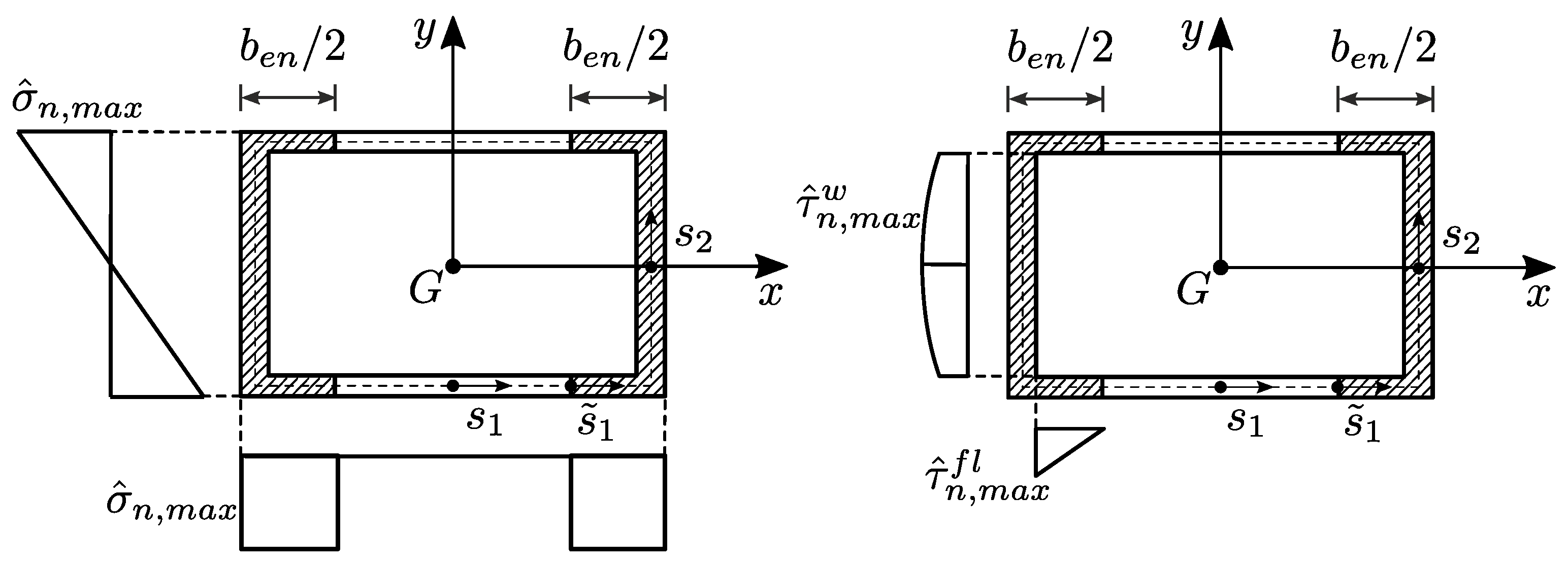The idea of this paper is to use such an n-depending effective to analyze static problems. Indeed, since any load can be expanded in a sinus Fourier series, it is possible to associate a different effective width to each of the harmonic components. By superimposing the effects, displacements and stresses, triggered by the original load, can be computed. The primary objective of this work is to evaluate, in each cross-section of the box-girder, the maximum value of the normal and tangential stresses. In particular, in each cross-section, the maximum normal stress occurs at the nodes, while maximum tangential stresses occur at the nodes of the flange and in the middle of the web. The proposed procedure, thanks to its user-friendliness, is intended as a valid alternative to consider the shear-lag effect in bridge designs.

Always in the framework of the Fourier analysis, the evaluation of displacements by using the Euler–Bernoulli beam model with the n-dependent inertia moment is proposed. Displacements by Euler–Bernoulli and Timoshenko beams with integer geometric characteristics are also illustrated for comparison.

Finally, the idea of an average effective width, which by still keeping the necessary dependence on the load shape avoids the need to employ a series expansion, is suggested here. This average effective width is intended as a medium value of the wavelength-dependent effective widths, and it can be obtained by imposing the equivalence of the displacements, or of the normal stresses, in a significant point of the beam.

The paper is organized as follows. In Section 2, the problem is defined, and the analytical expression derived in [35] for the effective flange width is recalled. In Section 3, making use of the reduced geometric characteristics, analytical expressions for both normal and tangential stresses are derived and discussed. In Section 4, always in the framework of the Fourier analysis, the deflections of the beam are evaluated by three different models of increasing refinement. In Section 5, the analytical formula for the average effective width for different load conditions is obtained and compared to the literature. In Section 6, displacements and stresses of a box-girder taken from the literature under different load conditions are evaluated by the present method and numerical results are discussed vs. Finite Element analyses. In Section 7, some conclusions are drawn.

2. Effective Flange Width

The formulation developed in [35] to obtain the effective flange width of rectangular box-girders undergoing sinusoidal deflections is summarized here.

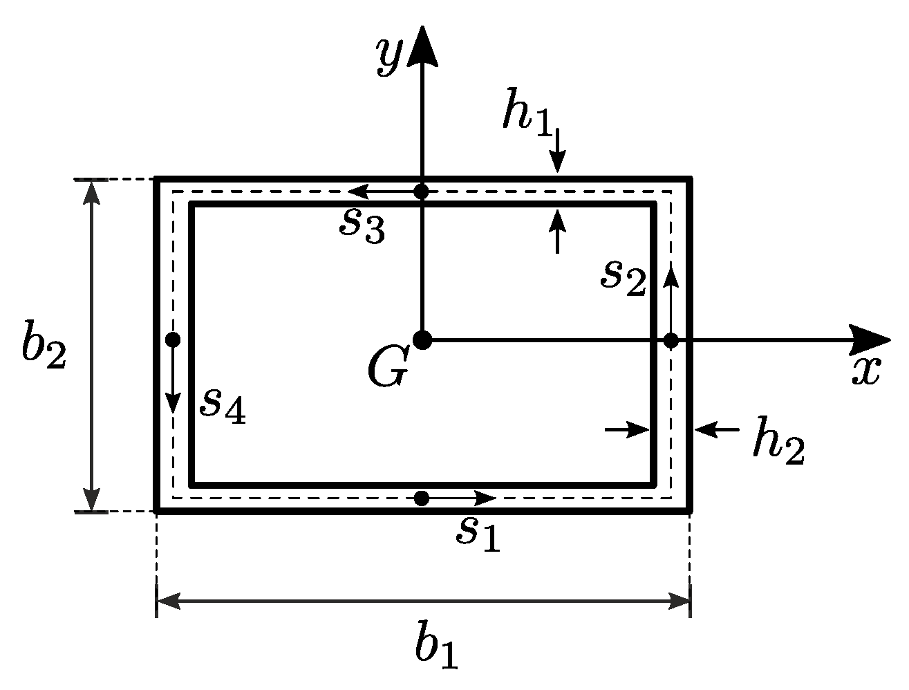
A double-symmetric box-girder of dimensions $b_1\times b_2$ and span $\mathcal{l}$, illustrated in Figure 1, is considered. The box-girder comprises four thin-walled elements: the bottom and upper flanges, represented by $i=1,3$ and having a thickness $h_1=h_3$, and the right and left webs, represented by $i=2,4$, and having a thickness $h_2=h_4$. The box-girder is referenced to the cross-section inertia principal axes $x,y$ at the centroidal axis $z\in \left(0,\mathcal{l}\right)$. The curvilinear abscissa are represented by $s_i\in \left(-\frac{b_i-h_2}{2},\frac{b_i-h_2}{2}\right)$ along the flanges and by $s_i\in \left(-\frac{b_i-h_1}{2},\frac{b_i-h_1}{2}\right)$ along the webs. Furthermore, the box-girder is simply supported and torsionally clamped at the ends. Additionally, the cross-section of the box-girder is assumed to remain undeformable within its own plane. In-plane displacements of the cross-section, along the $x,y$ axes, are denoted by $u,v$ respectively and out-of-plane displacements by w.

A simplified analytical model based on the following hypotheses is used: (a) the vertical deflection of the box-girder is sinusoidal; (b) the flange and the web are inextensible in the cross-section plane; and (c) the web is shear undeformable. It is assumed that the box-girder deflects in the $yz$ plane with a sinusoidal law

$$v\left(z\right)=\widehat{v}sin\left(\frac{n\pi }{\mathcal{l}}z\right)$$

(1)

of amplitude $\widehat{v}$. By virtue of the hypotesis (b), it is $u\left(z,s_i\right)=0$. The out-of-plane displacement of the bottom flange is taken as $w\left(z,s_1\right)=\widehat{w}\left(s_1\right)cos\left(\frac{n\pi }{\mathcal{l}}z\right)$, with aplitude $\widehat{w}\left(s_1\right)$ to be determined by equilibrium conditions together with symmetry considerations (the amplitude should be symmetric with respect to the y axis).

The membrane strains on the flange are written, and then, the active stresses in the flange are derived by the elastic law (taking zero, for the moment, the Poisson ratio). By enforcing the indefinite equilibrium in the z direction and integrating ordinary differential equations, the normal stresses are evaluated. Finally, the result of these abscissa-dependent stresses acting on the flange is equated to the product of the maximum stress occurring at the flange–web junction by the unknown effective width $b_{en}$. The following result is drawn:

$$b_{en}=\frac{2}{\beta }tanh\left(\frac{b_1}{2}\beta \right)$$

(2)

where

$$\beta :=\frac{n\pi }{\mathcal{l}}\sqrt{\frac{E}{G}}$$

(3)

is the wave number. The shear-lag coefficient ${\alpha }_n=\frac{b_{en}}{b_1}$ is defined as follows:

$${\alpha }_n=\frac{2}{n\pi \frac{b_1}{\mathcal{l}}\sqrt{\frac{E}{G}}}tanh\left(n\pi \frac{b_1}{2\mathcal{l}}\sqrt{\frac{E}{G}}\right)$$

(4)

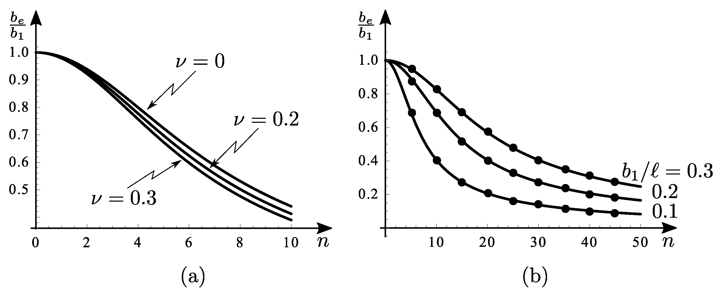
in which E and G are the Young modulus and the tangential elastic modulus, respectively. This is a ready-for-use formula, giving the effective width as a function of (i) the width-to-length ratio of the box-girder, (ii) the material property ratio $E/G=2\left(1+\nu \right)$, with $\nu$ the Poisson coefficient, and (ii) the number n of halfwaves which the beam deflects. For a beam of given geometric and mechanical characteristics, this latter is the only variable. 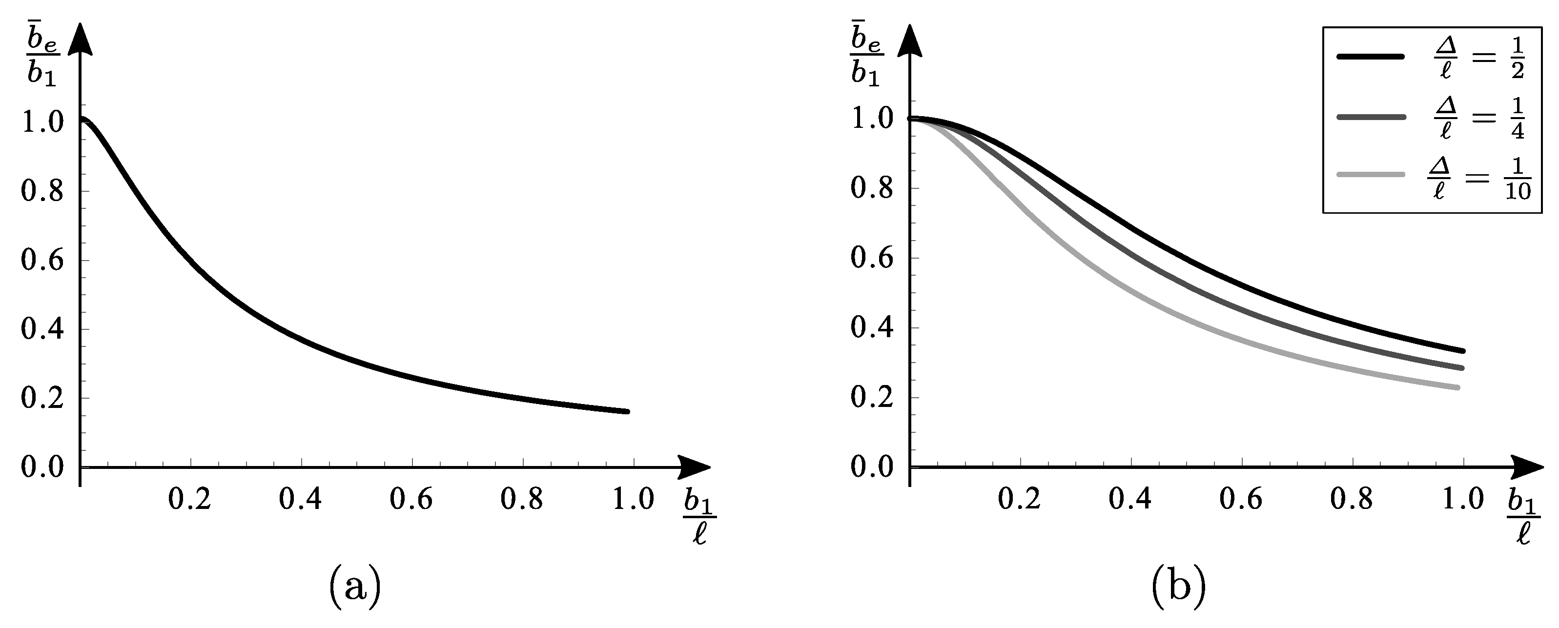The shear-lag coefficient in Equation (4) is plotted in Figure 2a vs. n, for a fixed $\frac{b_1}{\mathcal{l}}$ and different values of $\nu$. It is noticed that the material parameter weakly affects the results. Figure 2b shows the shear-lag coefficient vs. n, for different values of $\frac{b_1}{\mathcal{l}}$. For fixed $\frac{b_1}{\mathcal{l}}$, the graph makes it possible to associate with each n the corresponding value of $\frac{b_{en}}{b_1}$ and therefore the known $b_1$, the relevant $b_{en}$.

3. State of Stress

The statics of a simply supported box-girder subjected to vertical loads is studied here, with the purpose of evaluating the maximum normal and tangential stresses.

3.1. Load and Solicitation

The load $p\left(z\right)$ (positive upwards) is expanded in Fourier sine series as

$$p\left(z\right)=\sum _n{\widehat{p}}_{n}sin\left(\frac{n\pi }{\mathcal{l}}z\right)$$

(5)

where the Fourier coefficient ${\widehat{p}}_n$, representing the amplitude of the n-th harmonic, is given by

$${\widehat{p}}_n=\frac{2}{\mathcal{l}}\underset{0}{\overset{\mathcal{l}}{\int }}p\left(z\right)sin\left(\frac{n\pi }{\mathcal{l}}z\right)dz$$

(6)

To evaluate the shear force $T\left(z\right)$ and the bending moment $M\left(z\right)$, the equilibrium equations $T^{\prime }\left(z\right)+p\left(z\right)=0$, $M^{\prime }\left(z\right)+T\left(z\right)=0$ (shear force positive counterclockwise, bending moment positive when inducing upward concavity) must be integrated, with the boundary conditions $M\left(0\right)=M\left(\mathcal{l}\right)=0$. Here, a dash denotes differentiation with respect to z. Since the beam is isostatically constrained, this problem admits a unique solution, namely

$$\begin{array}{cc}\hfill T\left(z\right)& =\sum _n{\widehat{T}}_{n}cos\left(\frac{n\pi }{\mathcal{l}}z\right)\hfill \\ \hfill M\left(z\right)& =\sum _n{\widehat{M}}_{n}sin\left(\frac{n\pi }{\mathcal{l}}z\right)\hfill \end{array}$$

(7)

where the solicitation-amplitudes ${\widehat{T}}_n,{\widehat{M}}_n$ are related to the load-amplitudes by

$$\begin{array}{cc}\hfill {\widehat{T}}_n& =\frac{\mathcal{l}}{n\pi }{\widehat{p}}_n\hfill \end{array}$$

(8a)

$$\begin{array}{cc}\hfill {\widehat{M}}_n& =-{\left(\frac{\mathcal{l}}{n\pi }\right)}^2{\widehat{p}}_n\hfill \end{array}$$

(8b)

As an example, three cases are dealt with ahead (loads negative, since downward), namely, in Figure 3, (i) the uniformly distributed load $p\left(z\right)=-p_{0d}=\mathrm{const}$; (ii) the segment of uniform load $p_{0s}$ distributed on an interval $\left(\xi -\frac{\Delta }{2},\xi +\frac{\Delta }{2}\right)$, i.e., $p\left(z\right)=-p_{0s}W\left(\xi -\frac{\Delta }{2},\xi +\frac{\Delta }{2}\right)$, where $W\left(·\right)$ is the window function; and (iii) the concentrated load P applied at the abscissa $\xi$, i.e., $p\left(z\right)=-P\delta \left(z-\xi \right)$, where $\delta \left(·\right)$ is the Dirac function. In the three cases, the Fourier coefficients read, respectively,

$$\begin{array}{cc}\hfill {\widehat{p}}_n& =\frac{2p_{0d}\left(1-{\left(-1\right)}^n\right)}{n\pi }\hfill \end{array}$$

(9a)

$$\begin{array}{cc}\hfill {\widehat{p}}_n& =\frac{4p_{0s}}{n\pi }sin\left(\frac{\Delta n\pi }{2\mathcal{l}}\right)sin\left(\frac{\xi n\pi }{\mathcal{l}}\right)\hfill \end{array}$$

(9b)

$$\begin{array}{cc}\hfill {\widehat{p}}_n& =\frac{2}{\mathcal{l}}Psin\left(\frac{\xi n\pi }{\mathcal{l}}\right)\hfill \end{array}$$

(9c)

By using Equation (8), the relevant solicitation amplitudes are evaluated.

Both normal and tangential stress fields are obtained. These stresses are obtained here by using the De Saint Venant theory, in particular, the Navier theory is adopted for the normal stresses and the Jourawsky theory for the tangential ones.

3.2. Stresses

The normal stresses ${\sigma }_z\left(z,s\right)$ and the tangential stresses ${\tau }_{zs}\left(z,s\right)$, respectively, induced by the bending moment $M\left(z\right)$ and the shear force $T\left(z\right)$, are evaluated according to the technical theory of the beam, which extends the De Saint Venant results to beams loaded along their axis. Consequently, the Navier and the Jourawsky formulas are assumed to hold. However, to account for the shear-lag effects, reference must be made to the effective cross-section, in which the true width $b_1$ is replaced by the effective width $b_{en}=b_e\left(n\right)$, as illustrated in Figure 4. Due to the dependence on n, it is no possible to define an effective width of the flange valid for any loads, but reference has to be made to the single harmonic component of solicitation, i.e., ${\widehat{M}}_{n}sin\left(\frac{n\pi }{\mathcal{l}}z\right)$ and ${\widehat{T}}_{n}cos\left(\frac{n\pi }{\mathcal{l}}z\right)$ (which, indeed, trigger a sinusoidal deflection of the beam in n halfwaves). For each of these harmonics, the Navier and Jourawsky formulas are applied to a different geometry of the cross-section, and the stresses are added together to obtain

$$\begin{array}{c}\hfill {\sigma }_z\left(z,s\right)={\sum }_n{\widehat{\sigma }}_n\left(s\right)sin\left(\frac{n\pi }{\mathcal{l}}z\right)\end{array}$$

(10a)

$$\begin{array}{c}\hfill {\tau }_{zs}\left(z,s\right)={\sum }_n{\widehat{\tau }}_n\left(s\right)cos\left(\frac{n\pi }{\mathcal{l}}z\right)\end{array}$$

(10b)

where

$${\widehat{\sigma }}_n\left(s\right)=\frac{{\widehat{M}}_n}{I_n}y,{\tau }_{zs}\left(s\right)=-\frac{{\widehat{T}}_n}{I_{n}h\left(s\right)}{S}_n^{*}\left(s\right)$$

(11)

Here,

$$I_n=2\left({\left(\frac{b_2-h_1}{2}\right)}^2{b}_e{h}_1+\frac{1}{12}{h}_2{\left(b_2-2h_1\right)}^3+\frac{1}{12}{b}_e{h}_1^3\right)$$

(12)

is the second-order inertia moment (with respect to the x axis) of the effective rectangular box-girder associated with the n-th harmonic of the solicitation, i.e., to flanges of width $b_{en}=b_e\left(n\right)$. Similarly, $S_n^{*}\left(s\right)$ is the static moment of the portion of effective cross-section cuts by a chord at the abscissa s, reading

$$S_n^{*}\left(s_{1,2}\right)=\left\{\begin{array}{c}\begin{array}{cc}-{\tilde{s}}_1{h}_1\left(\frac{b_2-h_1}{2}\right),\hfill & {\tilde{s}}_1\in \left[0,\frac{b_{en}-h_2}{2}\right]\hfill \\ -\frac{h_1\left(b_2-h_1\right)\left(b_e-2h_2\right)}{4}-\frac{h_2}{8}\left(b_2^2-4b_2{h}_1+4h_1^2+\frac{s_2^2}{2}\right),\hfill & s_2\in \left[-\frac{b_2-h_1}{2},\frac{b_2-h_1}{2}\right],\hfill \end{array}\hfill \end{array}\right.$$

(13)

respectively, on the flange and on the web. Here, ${\tilde{s}}_1=s_1-\frac{b_1-b_{en}}{2}$ is a new translated abscissa.

The maximum (minimum) normal stress occurs at the top (bottom) of the cross-section, where, by using Equation (8b) in the Navier formula, it assumes the value

$${\widehat{\sigma }}_{n,max}=-{\left(\frac{\mathcal{l}}{n\pi }\right)}^2\frac{b_2}{2I_n}{\widehat{p}}_n$$

(14)

The relative maximum (in modulus) tangential stresses occur (i) on the flange, at the junction with the web (${\widehat{\tau }}_{n,max}^{fl}$), i.e., at ${\tilde{s}}_1=\frac{b_{en}}{2}-h_2,$ and (ii) on the web at the midpoint (${\widehat{\tau }}_{n,max}^w$), i.e., at $s_2=0$. By using Equation (8a) in the Jourawsky formula, they assume the values

$$\begin{array}{c}{\widehat{\tau }}_{n,max}^{fl}=\frac{\mathcal{l}}{n\pi }\frac{\left(b_2-h_1\right)\left(b_{en}-2h_2\right)}{4I_n}{\widehat{p}}_n\hfill \\ {\widehat{\tau }}_{n,max}^w=\frac{\mathcal{l}}{n\pi }\frac{1}{4I_n}\left(\frac{h_1\left(b_2-h_1\right)\left(b_e-2h_2\right)}{h_2}+\frac{{\left(b_2-2h_1\right)}^2}{2}\right){\widehat{p}}_n\hfill \end{array}$$

(15)

4. Displacements

To evaluate the deflections of the beam, three different models are used, of increasing refinement, and always in the framework of the Fourier analysis. The models are

• The total Euler–Bernoulli model ($E{B}_t$), in which the shear lag is ignored, so that the cross-section is the integer; this model is used only for comparison purposes, since it is expected it overestimates the stiffness of the beam;
• The total Timoshenko model ($T{M}_t$), in which the shear lag is still ignored, but the shear deformability of the web is accounted for by taking a shear area approximately equal to the web area, namely $A^{*}=A_{web}$; also this model is expected to give better results of the former, but they are still unsatisfactory;
• The effective Euler–Bernoulli model ($E{B}_e$), in which the shear-lag is included by exploiting the concept of wavelength-dependent effective width; this model is believed to be sufficiently accurate.

The shear lag could also be introduced in the Timoshenko model as, e.g., done in [35] in a dynamic context. There, it was proven that the Timoshenko model is more accurate than the Euler–Bernoulli model, when considering modes of short wavelength. In statics, however, since regular distribution of equiverse forces, which are of interest in bridge analysis, admit Fourier series in which higher harmonics bring a small contribution, the difference between the two models can be checked to be negligible, as proven ahead in the numerical analysis.

The $E{B}_t$ model is considered first. The equation of the elastic curve and boundary conditions of the simply supported beam read

$$\begin{array}{c}EI{v}^{\prime \prime \prime \prime }\left(z\right)=\sum _n{\widehat{p}}_{n}sin\left(\frac{n\pi }{\mathcal{l}}z\right)\hfill \\ v\left(0\right)=v\left(\mathcal{l}\right)=0\hfill \\ v^{″}\left(0\right)=v^{″}\left(\mathcal{l}\right)=0\hfill \end{array}$$

(16)

where $v\left(z\right)$ is the transverse displacement at the abscissa z, I is the second-order inertia moment of the integer cross-section and use has been made of Equation (5) to express the load. After integration, the following displacement field is found:

$$v\left(z\right)=\frac{{\mathcal{l}}^4}{{\pi }^{4}EI}\sum _n\frac{1}{n^4}{\widehat{p}}_{n}sin\left(\frac{n\pi }{\mathcal{l}}z\right)$$

(17)

Concerning, the $E{B}_e$ model, a different inertia moment must be taken for any n, so that the nth problem reads

$$\begin{array}{c}E{I}_n{v}_n^{\prime \prime \prime \prime }\left(z\right)={\widehat{p}}_{n}sin\left(\frac{n\pi }{\mathcal{l}}z\right)\hfill \\ v_n\left(0\right)=v_n\left(\mathcal{l}\right)=0\hfill \\ v_n^{″}\left(0\right)=v_n^{″}\left(\mathcal{l}\right)=0\hfill \end{array}$$

(18)

with $v_n\left(z\right)$ the response to the nth harmonic load component. From these equations, $v_n\left(z\right)={\widehat{v}}_{n}sin\left(\frac{n\pi }{\mathcal{l}}z\right)$ is found, with

$${\widehat{v}}_n=\frac{{\widehat{p}}_n}{E{I}_n}{\left(\frac{\mathcal{l}}{n\pi }\right)}^4$$

(19)

so that the response to $p\left(z\right)$, i.e., ${\sum }_n{\widehat{v}}_{n}sin\left(\frac{n\pi }{\mathcal{l}}z\right)$, is

$$v\left(z\right)=\frac{{\mathcal{l}}^4}{{\pi }^{4}E}\sum _n\frac{1}{n^4{I}_n}{\widehat{p}}_{n}sin\left(\frac{n\pi }{\mathcal{l}}z\right)$$

(20)

The solutions in Equations (17) and (20) are similar, but while the inertia I is the same in each term of the former series, the inertia $I_n$ decreases with the number n in each term of the latter series. Therefore, the $E{B}_e$ is softer than the $E{B}_t$ model.

Finally, the $T{M}_t$ model is addressed. The equilibrium equations in terms of the (independent) transverse displacement $v\left(z\right)$ and rotation $\phi \left(z\right)$ are (see, e.g., [35])

$$\begin{array}{c}-G{A}^{*}\left(v^{″}-{\phi }^{\prime }\right)=\sum _n{\widehat{p}}_{n}sin\left(\frac{n\pi }{\mathcal{l}}z\right)\hfill \\ -EI{\phi }^{″}-G{A}^{*}\left(v^{\prime }-\phi \right)=0\hfill \end{array}$$

(21)

with the boundary conditions

$$\begin{array}{c}\hfill v\left(0\right)=v\left(\mathcal{l}\right)=0\\ \hfill {\phi }^{\prime }\left(0\right)={\phi }^{\prime }\left(\mathcal{l}\right)=0\end{array}$$

(22)

and symbols already introduced. These equations are exactly solved by the series as follows:

$$\begin{array}{c}v\left(z\right)=\sum _n{\widehat{v}}_{n}sin\left(\frac{n\pi }{\mathcal{l}}z\right)\hfill \\ \phi \left(z\right)=\sum _n{\widehat{\phi }}_{n}cos\left(\frac{n\pi }{\mathcal{l}}z\right)\hfill \end{array}$$

(23)

whose coefficients are found to be

$$\begin{array}{cc}\hfill {\widehat{v}}_n& =\frac{{\widehat{p}}_n}{EI}{\left(\frac{\mathcal{l}}{n\pi }\right)}^4\left(1+\frac{EI}{G{A}^{*}}{\left(\frac{n\pi }{\mathcal{l}}\right)}^2\right)\hfill \\ \hfill {\widehat{\phi }}_n& =\frac{{\widehat{p}}_n}{EI}{\left(\frac{\mathcal{l}}{n\pi }\right)}^3\hfill \end{array}$$

(24)

Equation (24) shows that $G{A}^{*}<\infty$ amplifies the deflection, when compared to the $E{B}_e$ model (which corresponds to $G{A}^{*}=\infty$).

5. Average Effective Width

The theory developed so far explained that the effective width $b_{en}$ is strictly related to the load shape as well as the wavelengths of its harmonic components. However, one might want to obtain an approximate formula which, still keeping the necessary dependence on the load shape, avoids the need to employ a series expansion, which entails the simple but tedious addition of a larger number of contributions. In this perspective, the idea of an average effective width, obtained as a medium value of the wavelength-dependent effective widths, would be desirable.

5.1. Displacement Equivalence

To obtain such an average value, the following strategy is followed: (a) for a given load $p\left(z\right)$, the deflection at the midspan (or at another significant point) is computed via the proposed algorithm, through the series expansion Equation (20), i.e.,

$$v\left(\frac{\mathcal{l}}{2}\right)=\frac{{\mathcal{l}}^4}{{\pi }^{4}E}\sum _n\frac{1}{n^4{I}_n}{\widehat{p}}_{n}sin\left(\frac{n\pi }{2}\right);$$

(25)

(b) such a the displacement is equated to $\overline{v}\left(\frac{\mathcal{l}}{2}\right)$,experienced by a beam whose cross-section has flanges of average effective width ${\overline{b}}_e$, i.e., average inertia moment $\overline{I}$; (c) from the equality $\overline{v}\left(\frac{\mathcal{l}}{2}\right)=v\left(\frac{\mathcal{l}}{2}\right)$, the unknown ${\overline{b}}_e$ is derived.

The procedure is explained in detail for the case of uniformly distributed load $p\left(z\right)=p_{0d}=\mathrm{const}$, for which ${\widehat{p}}_n$ is given by Equation (9a). Since the midspan displacement of a beam of inertia moment $\overline{I}$, under the same load, is $\overline{v}\left(\frac{\mathcal{l}}{2}\right)=\frac{5}{384}\frac{p_{0d}{\mathcal{l}}^4}{E\overline{I}}$, by enforcing the equality, the unknown $\overline{I}$ is derived as

$$\overline{I}=\frac{5}{768}\frac{{\pi }^5}{{\sum }_n\frac{1}{I_n}\frac{\left(1-{\left(-1\right)}^n\right)}{n^5}sin\left(\frac{n\pi }{2}\right)}$$

(26)

Such an expression is still too complicated to draw ${\overline{b}}_e$, so that another strong simplification is introduced. It is assumed (only to the scope at hand) that the inertia moment of the reduced cross sections is almost equal to that of the two flanges (i.e., by neglecting the web contributions), whose area is concentrated in their centroids. Accordingly, $\overline{I}\simeq \frac{1}{2}{\overline{b}}_e{h}_1{\left(b_2-h_1\right)}^2$ and $I_n=\frac{1}{2}{b}_{en}{h}_1{\left(b_2-h_1\right)}^2$ so that the previous equation provides

$$\frac{{\overline{b}}_e}{b_1}=\frac{5}{768}\frac{{\pi }^5}{{\sum }_n\frac{\left(1-{\left(-1\right)}^n\right)}{n^5{\alpha }_n}sin\left(\frac{n\pi }{2}\right)}$$

(27)

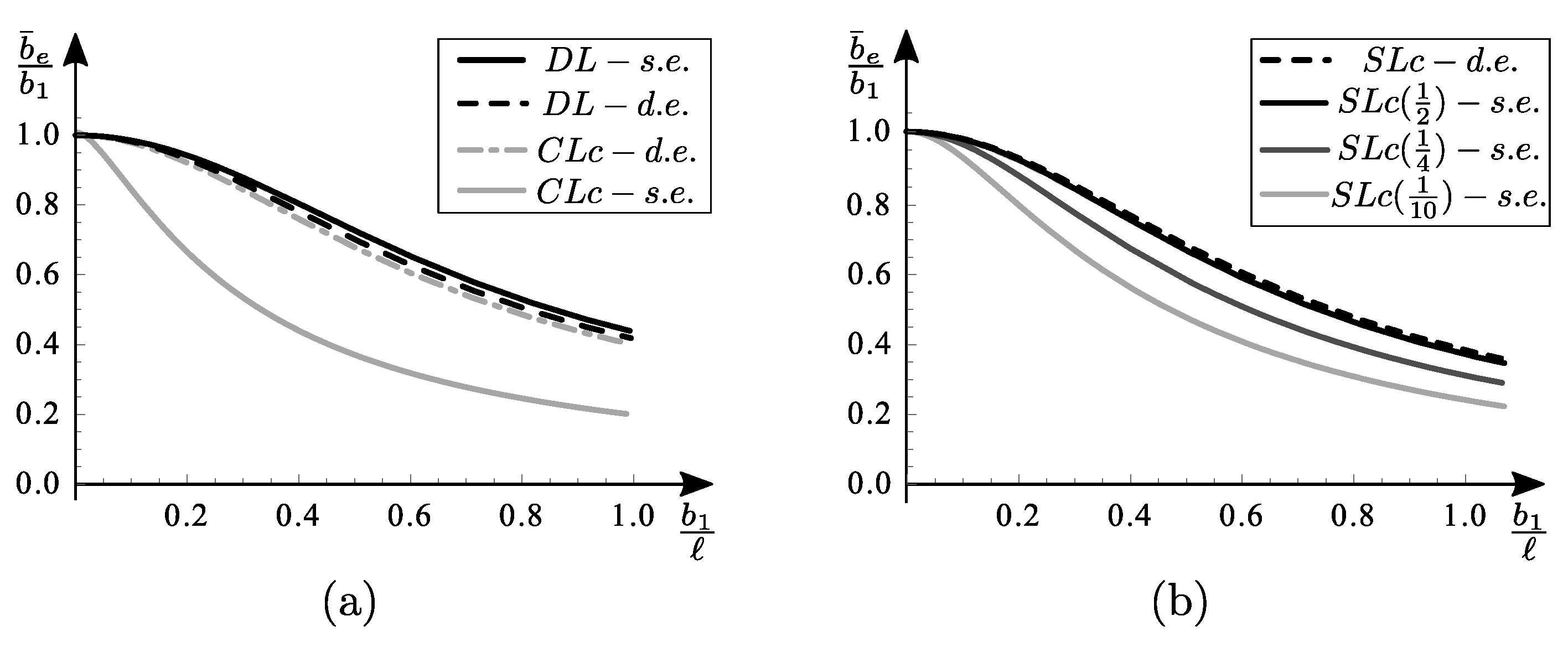
in which $b_{en}={\alpha }_n{b}_1$ has been introduced. By remembering Equation (4) for ${\alpha }_n$, it is concluded that $\frac{{\overline{b}}_e}{b_1}$ depends on the aspect ratio $\frac{b_1}{\mathcal{l}}$ and (weakly) on the Poisson ratio. By fixing the latter, a plot of $\overline{\alpha }=\frac{{\overline{b}}_e}{b_1}$ vs. $\frac{b_1}{\mathcal{l}}$ can be constructed (see Figure 5a), which is ready for use. Indeed, from known ${\overline{b}}_e$, the (now not approximated) inertia moment $\overline{I}$ can be computed, and stresses and displacements evaluated, without resorting to series expansions. The accuracy of this simplified method is tested in the next section.

By repeating the procedure for the concentrated load applied at the midspan (Figure 5a), it is found that

$$\frac{{\overline{b}}_e}{b_1}=\frac{1}{96}\frac{{\pi }^4}{{\sum }_n\frac{1}{n^4{\alpha }_n}{sin}^2\left(\frac{n\pi }{2}\right)}$$

(28)

and for a segment of load of extension $\Delta$ centered at the midspan (Figure 5b),

$$\frac{{\overline{b}}_e}{b_1}=\frac{1}{1536}\frac{{\pi }^5\left(8{\mathcal{l}}^3\Delta -4\mathcal{l}{\Delta }^3+{\Delta }^4\right)}{{\mathcal{l}}^4{\sum }_n\frac{1}{n^5{\alpha }_n}sin\left(\frac{\Delta n\pi }{2\mathcal{l}}\right){sin}^2\left(\frac{n\pi }{2}\right)}$$

(29)

5.2. Normal Stresses Equivalence

It is also possible to obtain an average value of the effective width by using the equivalence of the normal stresses instead of the displacements (Section 5.1). For this purpose, the following strategy, similar to that pursued in Section 5.1, is followed: (a) for a given load $p\left(z\right)$, the maximum normal stress at the midspan (or at another significant point) is computed via the proposed algorithm, through the series expansion Equation (10a), i.e.,

$${\sigma }_z\left(\frac{\mathcal{l}}{2},-\frac{b_2}{2}\right)=\frac{{\mathcal{l}}^2{b}_2}{2{\pi }^2}\sum _n\frac{1}{n^2{I}_n}{\widehat{p}}_{n}sin\left(\frac{n\pi }{2}\right)$$

(30)

(b) such a normal stress is equated to ${\overline{\sigma }}_z\left(\frac{\mathcal{l}}{2},-\frac{b_2}{2}\right)$,experienced by a beam whose cross-section has flanges of average effective width ${\overline{b}}_e$, i.e., average inertia moment $\overline{I}$; (c) from the equality ${\overline{\sigma }}_z\left(\frac{\mathcal{l}}{2},-\frac{b_2}{2}\right)={\sigma }_z\left(\frac{\mathcal{l}}{2},-\frac{b_2}{2}\right)$, the unknown ${\overline{b}}_e$ is derived.

In the three cases, uniformly distributed load, segment of load centered at the midspan and concentrated load applied at the midspan, the normal stresses ${\overline{\sigma }}_z\left(\frac{\mathcal{l}}{2},-\frac{b_2}{2}\right)$ read, respectively,

$$\begin{array}{c}{\overline{\sigma }}_z\left(\frac{\mathcal{l}}{2},-\frac{b_2}{2}\right)=\frac{p_{0d}{\mathcal{l}}^2{b}_2}{16\overline{I}}\hfill \\ {\overline{\sigma }}_z\left(\frac{\mathcal{l}}{2},-\frac{b_2}{2}\right)=\frac{p_{0s}\Delta \left(2\mathcal{l}-\Delta \right)b_2}{16\overline{I}}\hfill \\ {\overline{\sigma }}_z\left(\frac{\mathcal{l}}{2},-\frac{b_2}{2}\right)=\frac{P\mathcal{l}{b}_2}{8\overline{I}}\hfill \end{array}$$

(31)

In the three cases, it is found, respectively, that

$$\begin{array}{c}\frac{{\overline{b}}_e}{b_1}=\frac{1}{16}\frac{{\pi }^3}{{\sum }_n\frac{\left(1-{\left(-1\right)}^n\right)}{n^3{\alpha }_n}sin\left(\frac{n\pi }{2}\right)}\hfill \\ \frac{{\overline{b}}_e}{b_1}=\frac{1}{32}\frac{{\pi }^3\Delta \left(2\mathcal{l}-\Delta \right)}{{\mathcal{l}}^2{\sum }_n\frac{1}{n^3{\alpha }_n}sin\left(\frac{\Delta n\pi }{2\mathcal{l}}\right){sin}^2\left(\frac{n\pi }{2}\right)}\hfill \\ \frac{{\overline{b}}_e}{b_1}=\frac{1}{8}\frac{{\pi }^2}{{\sum }_n\frac{1}{n^2{\alpha }_n}{sin}^2\left(\frac{n\pi }{2}\right)}\hfill \end{array}$$

(32)

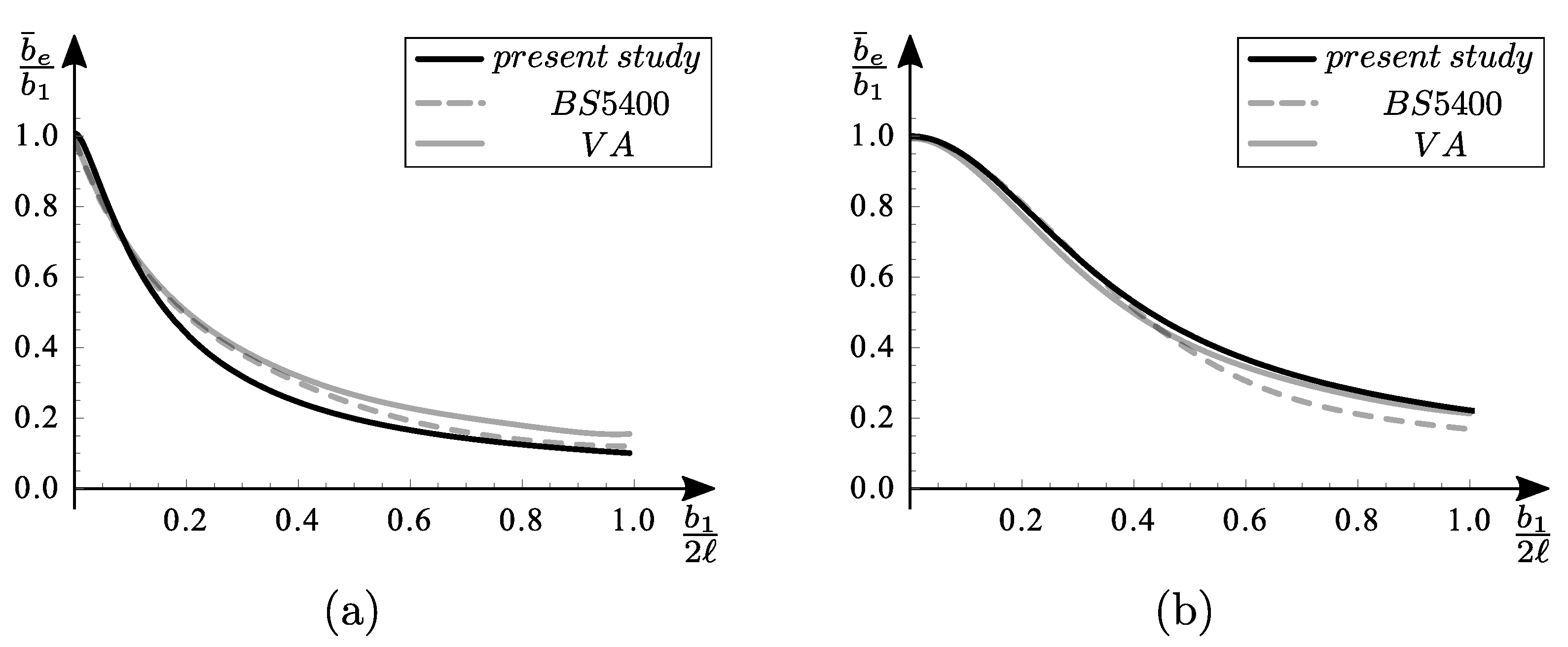
Figure 5 shows the average shear-lag coefficient $\overline{\alpha }=\frac{{\overline{b}}_e}{b_1}$ vs. $\frac{b_1}{\mathcal{l}}$ for the uniformly distributed load, concentrated load at the midspan and segment of distributed load, centered at midspan, for different extensions $\frac{\Delta }{\mathcal{l}}=\frac{1}{10},\frac{1}{4},\frac{1}{2}$, by both the displacement equivalence (dashed line) and the stresses equivalence (continuous line). Results obtained by the displacement equivalence does not appear able to take into account the loading conditions, therefore it is considered to be not sufficiently accurate.

The shear-lag coefficient for the two load cases, concentrated force at midspan and uniformly distributed load, have been studied by the BS5400 [34] and by a variational analysis in [27], where the graph of the shear-lag coefficient $\frac{b_e}{b_1}$ vs. $\frac{b_1}{2\mathcal{l}}$ is obtained numerically. Figure 6 shows results by BS5400, by [27] and by the present study all together, for the two load cases mentioned above. They are very close to each other; however, it is important to underline that our study, unlike the other studies mentioned, provides an analytical formula for the relationship, and therefore, it is applicable to different load conditions, and this character of generality constitutes an added value.

In support of the above, the calculation of the average shear-lag coefficient using the equivalence of the normal stresses for two load conditions not present in the literature is proposed here: a concentrated force applied at $\xi =\frac{\mathcal{l}}{4}$ and a segment of distributed load, centered at the abscissa $\xi =\frac{\mathcal{l}}{4}$. By following the procedure already described for the simplest loading conditions, in the new load cases considered, the normal stresses ${\overline{\sigma }}_z\left(\frac{\mathcal{l}}{4},-\frac{b_2}{2}\right)$ read, respectively,

$$\begin{array}{c}{\overline{\sigma }}_z\left(\frac{\mathcal{l}}{4},-\frac{b_2}{2}\right)=\frac{3}{32}\frac{P\mathcal{l}{b}_2}{\overline{I}}\hfill \\ {\overline{\sigma }}_z\left(\frac{\mathcal{l}}{4},-\frac{b_2}{2}\right)=\frac{p_{0s}\Delta \left(3\mathcal{l}-2\Delta \right)b_2}{32\overline{I}}\hfill \end{array}$$

(33)

So it is found, respectively, that

$$\begin{array}{c}\frac{{\overline{b}}_e}{b_1}=\frac{3}{32}\frac{{\pi }^2}{{\sum }_n\frac{1}{n^2{\alpha }_n}{sin}^2\left(\frac{n\pi }{4}\right)}\hfill \\ \frac{{\overline{b}}_e}{b_1}=\frac{1}{64}\frac{{\pi }^3\Delta \left(3\mathcal{l}-2\Delta \right)}{{\mathcal{l}}^2{\sum }_n\frac{1}{n^3{\alpha }_n}sin\left(\frac{\Delta n\pi }{2\mathcal{l}}\right){sin}^2\left(\frac{n\pi }{4}\right)}\hfill \end{array}$$

(34)

Figure 7 shows the average shear-lag coefficient $\overline{\alpha }$ vs. $\frac{b_1}{\mathcal{l}}$ for the concentrated load applied at $\xi =\frac{\mathcal{l}}{4}$ and for the segment of the distributed load, centered at the abscissa $\xi =\frac{\mathcal{l}}{4}$, for different extensions $\frac{\Delta }{\mathcal{l}}=\frac{1}{10},\frac{1}{4},\frac{1}{2}$.

6. Numerical Results

The theory so far developed is applied, for validation purposes, to perform the static analysis of sample simple-supported box-girders in bending, for which the analytical results are compared with those supplied by Finite Element analyses. A case study is considered, consisting of a reinforced concrete box-girder bridge taken from the literature [36]. Three different load cases are analyzed: (i) a uniformly distributed load $p_{0d}$ (DL); (ii) a segment of uniformly distributed load $p_{0s}$ (SL) on a length $\Delta =\frac{\mathcal{l}}{4}$, centered at the abscissa $\xi =\frac{\mathcal{l}}{4}$ and (iii) a concentrated load P (CL) applied at $\xi =\frac{\mathcal{l}}{4}$.

The FEM analysis utilized a commercial software, namely SAP2000. The structural representation of the box bridge involves the assembly of thin-shell elements. To realize the boundary conditions of the analytical model, the in-plane displacements of all mesh nodes are constrained at the end cross-sections. Additionally, at one end, the longitudinal displacement of two points along the x-axis is restricted and ’diaphragm constraints’ at every cross-section of the mesh are introduced to simulate the non-deformability of all the cross-sections of the girder, allowing for unrestricted flexural warping.

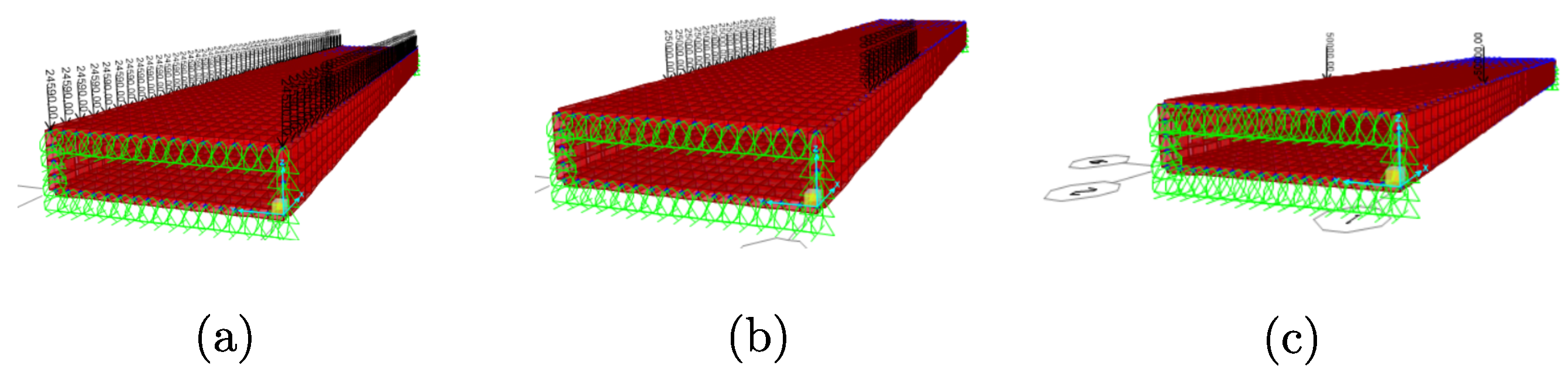
Regarding the application of loads in the FE model, it is important to note that it exclusively employs thin-shell elements. Consequently, loads can only be applied at joints as concentrated loads using the ‘Assign joint loads’ command. The selected joints for applying forces are located at the intersections of webs (elements 2, 4) and the top flange (element 3) as shown in Figure 8. This choice is justified by the usual procedure carried out in the bridge analysis, in which the loads applied to the flange are “brought to the nodes” by performing first a “local effect analysis”, in which the nodes are fictitiously supported, and successively a “global effect analysis”, in which the reactive forces, changed in sign, are applied to the nodes, freed from constraints.

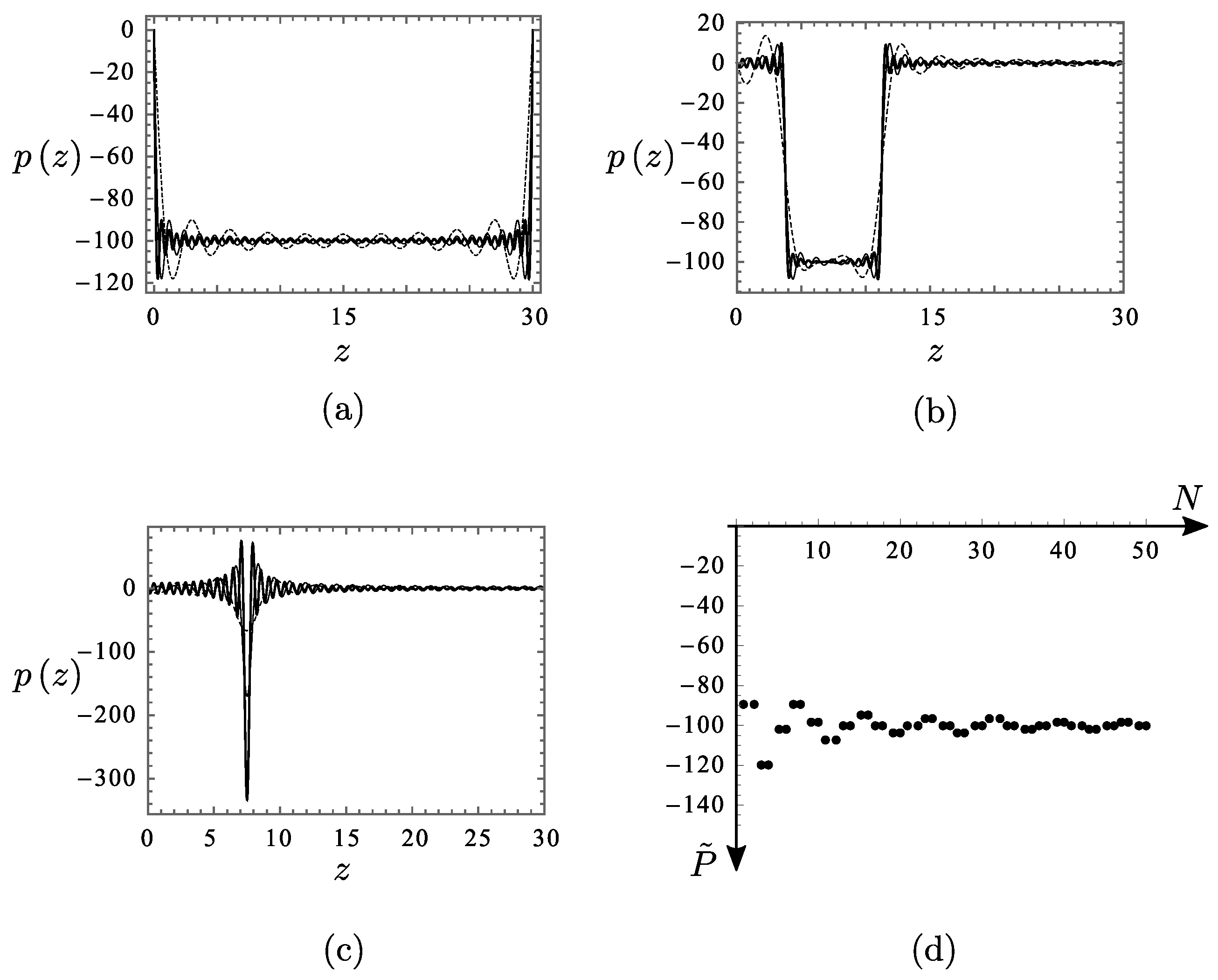
Chosen $p_{0d}=p_{0s}=p_0=-100\mathrm{kN}/\mathrm{m}$, $P=-100\mathrm{kN}$, the loads DL, SL and CL are expressed as sinusoidal Fourier series and depicted in Figure 9 for $N=20,50,100$. To determine an appropriate value for N, Fourier analyses are conducted for increasing values of this number. The Fourier series with $N=20$ inadequately approximates the loads, particularly in the SL case and, even worse, in the CL case (see Figure 9). For the last case, in particular, it was deemed useful to carry out a convergence analysis of $\tilde{P}={\int }_0^{\mathcal{l}}p\left(z\right)dz$ (Figure 9d). Consequently, $N=50$ is ultimately selected for the analysis.

6.1. Case Study

A rectangular box-girder bridge, made of reinforced concrete, is considered as a case study, as detailed in [36]. The geometric specifications of the box-girder are as follows: length $\mathcal{l}=30\mathrm{m}$, width $b_1=6.35\mathrm{m}$, height $b_2=1.75\mathrm{m}$, flange thickness $h_1=0.25\mathrm{m}$, and web thickness $h_2=0.35\mathrm{m}$ (refer to Figure 1). The elastic modulus is $E=\mathrm{35,654}\times {10}^3\mathrm{kN}/{\mathrm{m}}^2$, and the Poisson’s coefficient is $\nu =0.15$. The mass per unit volume is calculated as $\rho =\frac{\mathrm{25,000}}{9.81}=2548.42\mathrm{kg}/{\mathrm{m}}^3$.

The Finite Element analysis involved the utilization of a model comprising 2400 shell elements (40 along the directrix and 60 along the axis). This resulted in a total of 2440 degrees of freedom. In this FE model, the side of the mesh is $d=0.5\mathrm{m}$, so for the uniformly distributed load (DL), the number of joints, in correspondence with each web, where the force must be applied is $n_{DL}=(\frac{\mathcal{l}}{d}+1)=61$, and the modulus of any concentrated force is $\frac{p_0\times \mathcal{l}}{2n_{DL}}=24.59\mathrm{kN}$ (see Figure 8a). For the segment of uniformly distributed load (SL), a similar but different mode of working, based on the concept of area of influence, is chosen as follows: at $n_{SL}=\frac{\Delta }{d}=15$ joints in correspondence with each web (the first located at $z=4\mathrm{m}$), the concentrated force $\frac{p_0\times \Delta }{2n_{SL}}=25\mathrm{kN}$ is applied (see Figure 8b). The concentrated load is applied as a concentrated force $\frac{P}{2}=50\mathrm{kN}$ at the joint located at $z=7.5\mathrm{m}$ in correspondence with each web (see Figure 8c).

6.1.1. Stress Analysis

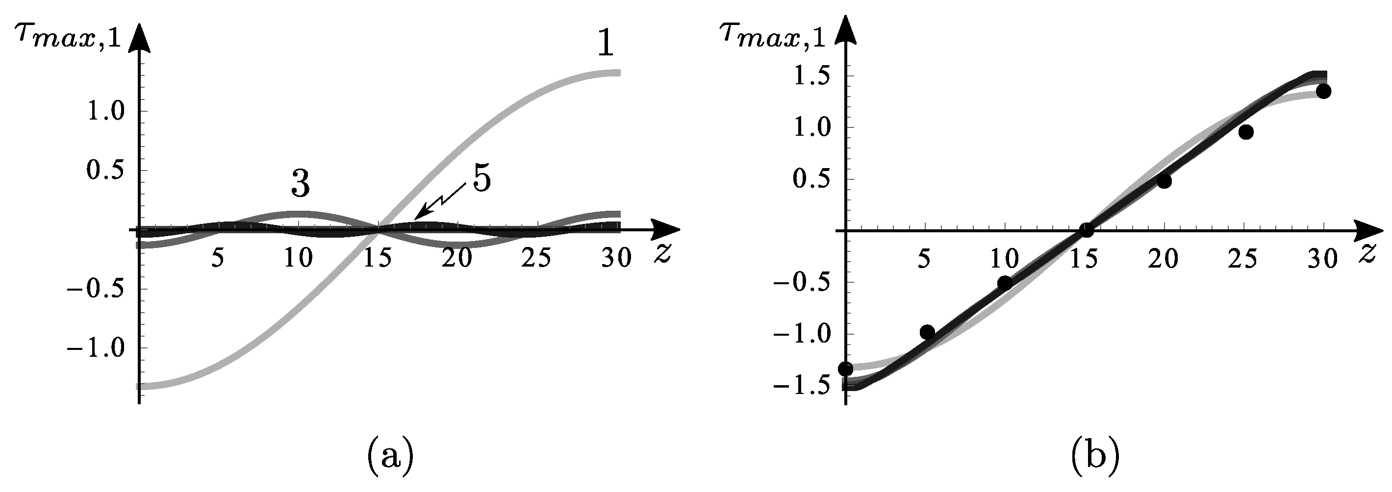
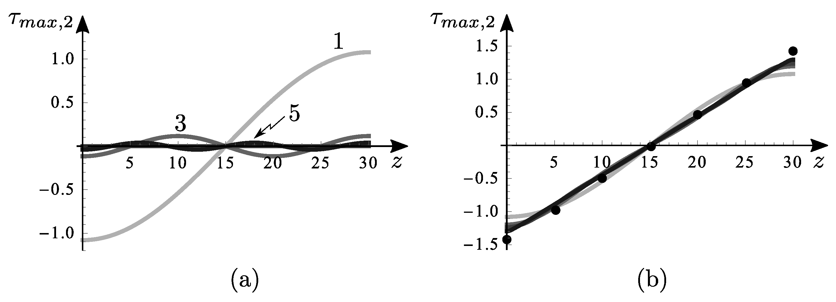
Maximum normal and tangential stresses (Equations (14) and (15)), at different cross-sections, are plotted in Figure 10, Figure 11 and Figure 12 for the uniformly distributed load case (DL). In particular, Figure 10b–Figure 12b show the maximum stresses for different N both by analytical and numerical models (taken as a reference), revealing a fast convergence, also for low n.

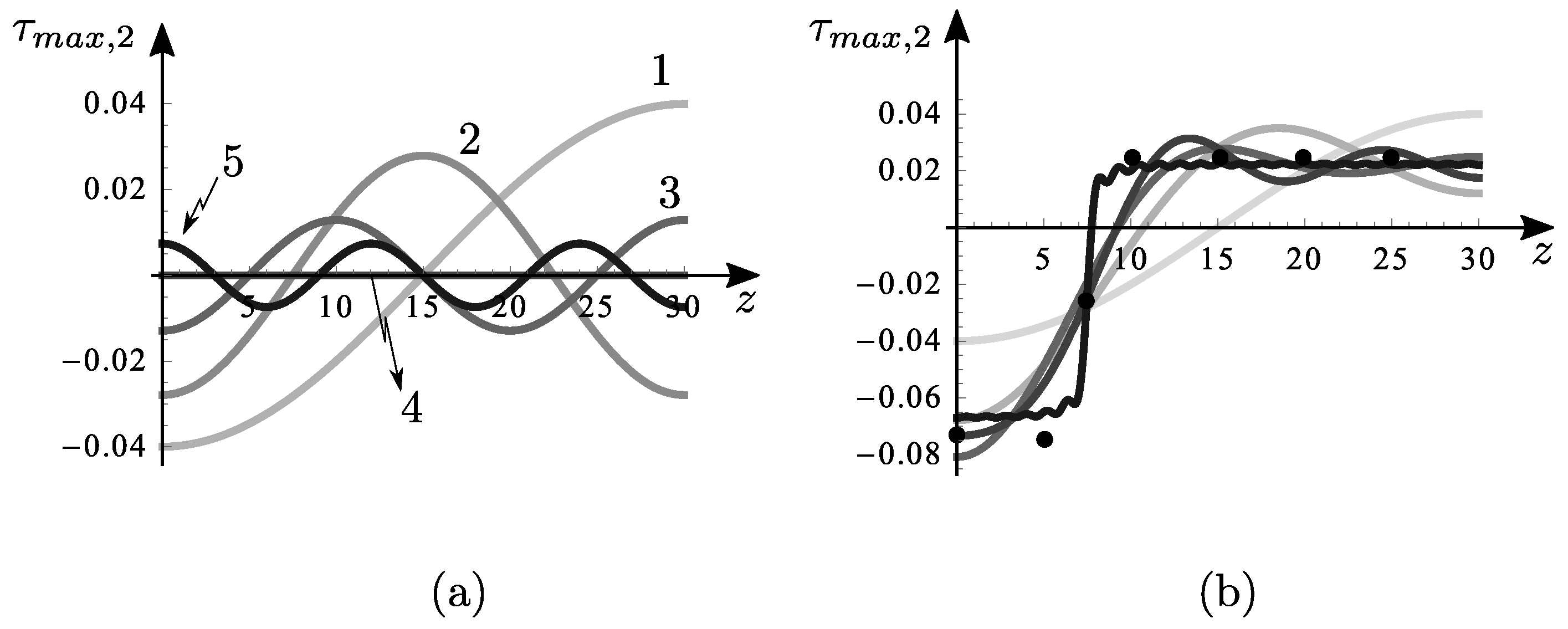
In order to set the sufficient number of harmonics to use, an analysis of harmonics for the stresses on z is carried out. Figure 10a–Figure 12a indicate that starting from $n=5$, the influence of the pertinent harmonic becomes negligible. Consequently, it can be inferred that conducting a Fourier analysis with an $N=50$ would be futile. As previously elucidated, the decision to employ a Fourier series with $N=50$ has been made to effectively approximate the loads, particularly the loaded segment.

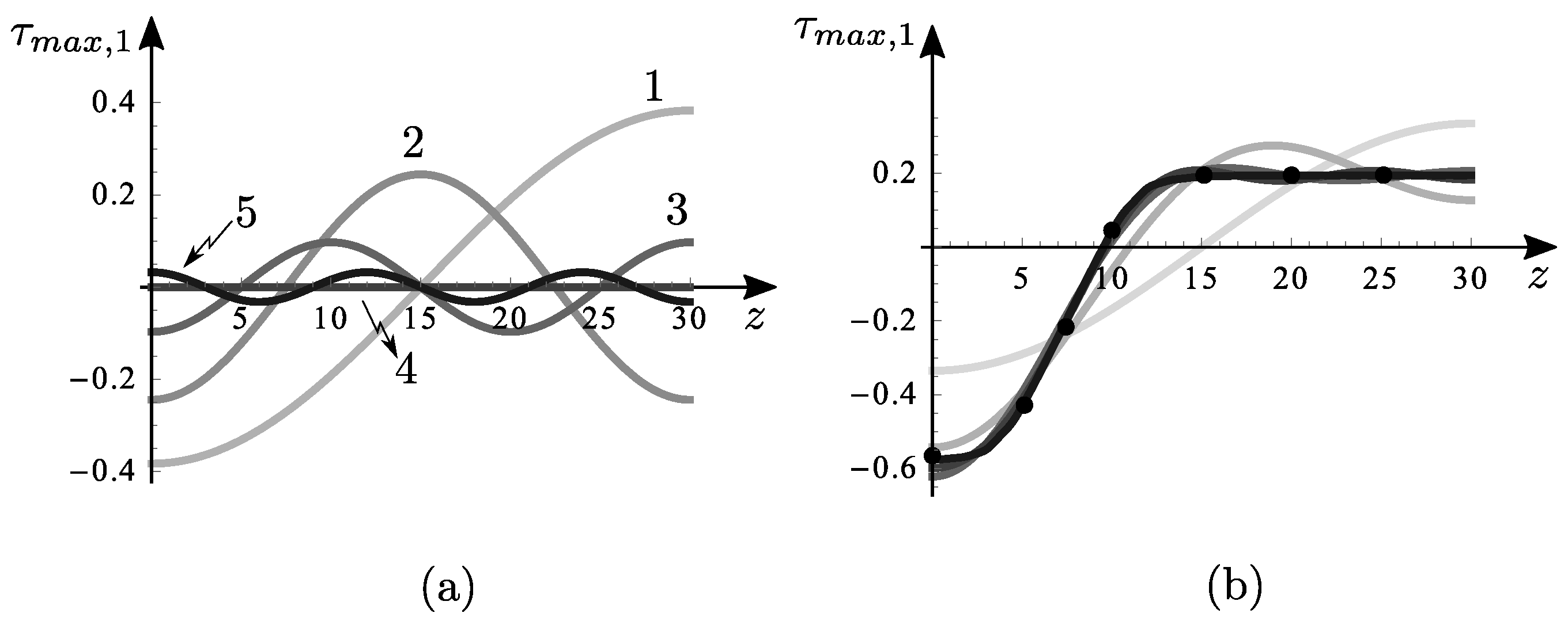
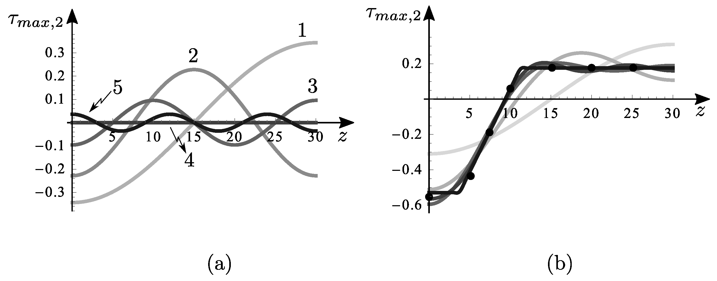
Figure 13, Figure 14 and Figure 15 are about the segment of uniformly distributed load (SL). Similar considerations to the previous case can be made.

Figure 16, Figure 17 and Figure 18 are about the concentrated load (CL). In this case, it is particularly important to consider $N=50$ instead of smaller N to capture a stress value sufficiently close to the FE model, especially in correspondence with the concentrated load (see Figure 16b) with a maximum error of about 5% for the maximum normal stresses and 12% for the maximum tangential stresses.

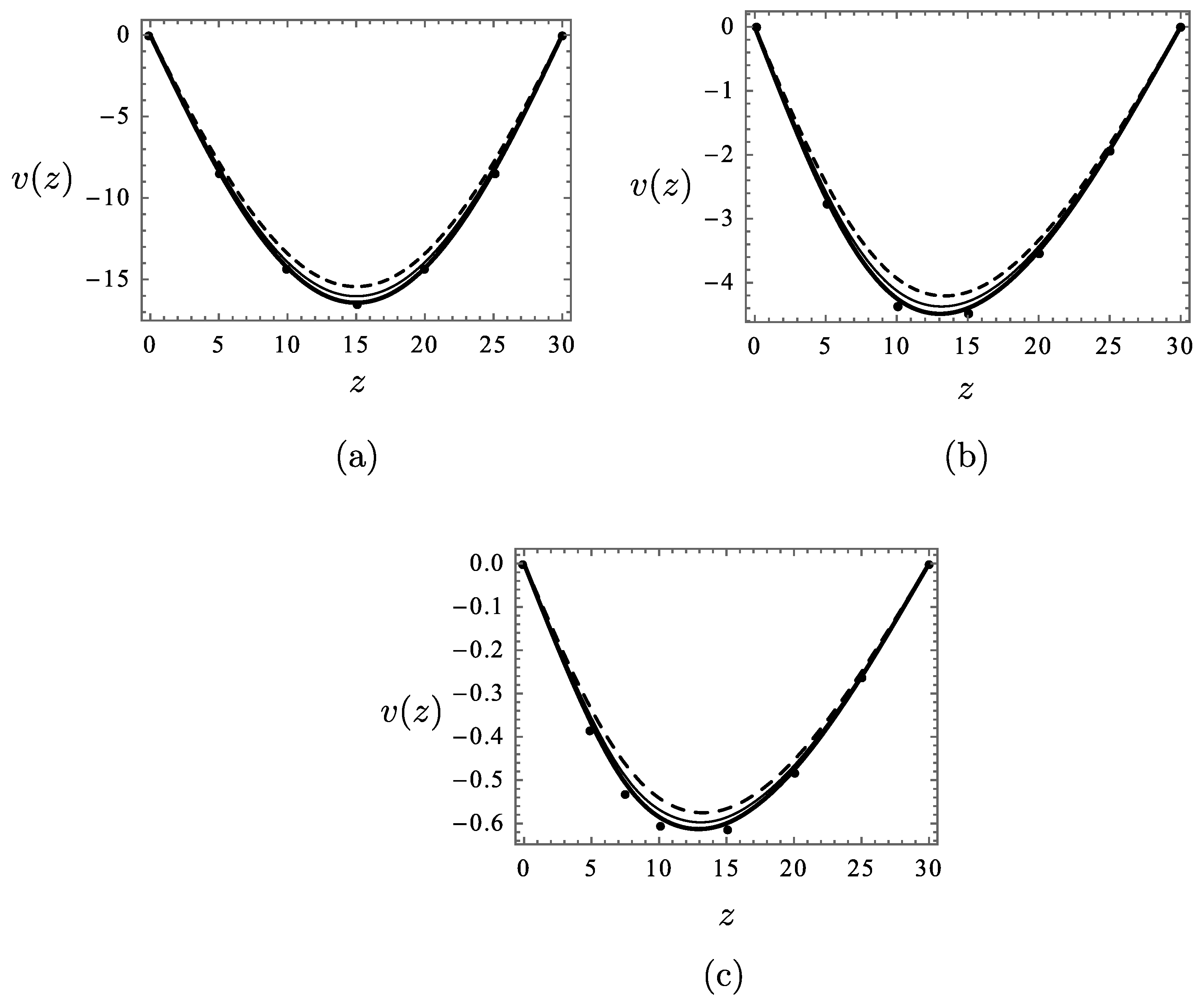
6.1.2. Displacement Analysis

The vertical displacement $v\left(z\right)$ by the three analytical models considered (total Euler-Bernoulli, total Timoshenko and effective Euler-Bernoulli) are plotted in Figure 19 with those by the FEM analysis, for the three load cases. As expected, for all three cases analyzed, the $E{B}_e$ model, in which the shear-lag is included by exploiting the concept of wavelength-dependent effective width, is the most consistent with the FEM results with a maximum error of about 0% for the DL, 1.6% for the SL and 2.8% for the CL. Furthermore, $E{B}_t$ and $T{M}_t$ model present respectively a maximum error of about 7% and 3.6% for the DL, 8.7% and 2% for the SL, and 8.9% and 5.3% for the CL.

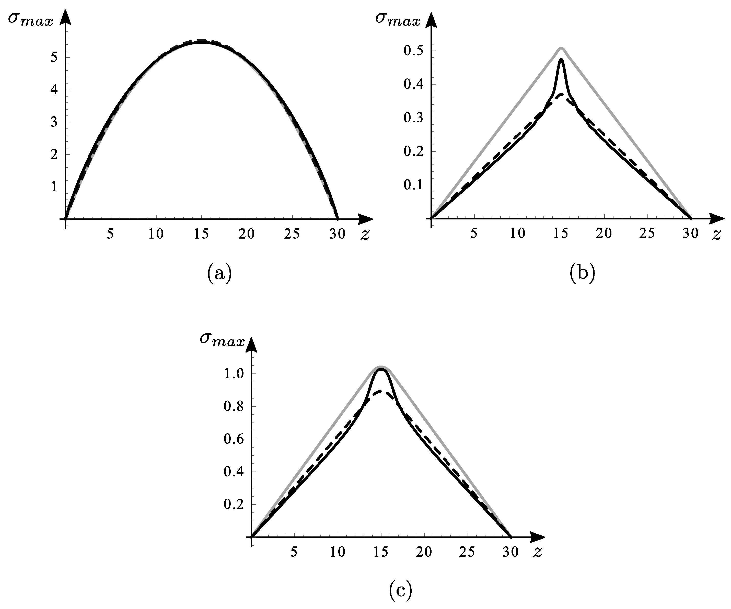
6.1.3. Use of the Average Effective Width

The goodness of the results obtained by using the effective width $b_{en}$ has already been tested by comparison with FEM results, so it is now intended to compare the normal stresses obtained by considering the effective width $b_{en}$ by Equation (2), taken as a reference, with those by considering the average effective width ${\overline{b}}_e$ derived both from the displacement equivalence and the normal stress equivalence (see Section 5). For this comparison, the three simple loading conditions already mentioned in Section 5 are considered, in particular, the uniformly distributed load $p_{0d}=-100\mathrm{kN}/\mathrm{m}$ (DL), the segment of load $p_{0s}=-100\mathrm{kN}/\mathrm{m}$ of extension $\Delta =\frac{\mathcal{l}}{10}$ centered at midspan (SL-centered) and concentrated load $P=-100\mathrm{kN}$ applied at midspan (CL-centered).

Figure 20 shows that for the DL case, the three curves are almost superimposed, while, on the contrary, for the CL-centered case, the two curves related to the average effective widths are notably different; in particular, deriving from the normal stresses equivalence captures the maximum value quite well, while deriving from the displacement equivalence follows the curve better but is not able to approximate the maximum value. The case of SL-centered is an intermediate case. The amount of the difference between the two approximate curves depends on the extension $\Delta$ of the segment loaded.

7. Conclusions

A new method has been proposed for the bending static analysis of simply supported, but generally loaded, rectangular box-girders with undeformable cross-section, undergoing shear-lag. The method is based on (i) expanding the general load in the Fourier series; (ii) finding the effective flange width relevant to each harmonic; (iii) computing, for each harmonic, displacements and stresses by using a beam model with effective geometric characteristics; and (iv) combining the results of all the harmonics. As an alternative to the effects combination, approximate formulae giving ready-for-use expressions for an “average effective width” have been derived, based on equivalences at selected points with (i) displacements or (ii) stresses of the more refined model. Results have been compared with much more expensive Finite Element analyses to validate the method presented. The following conclusions, relevant to sample loading conditions, have been drawn.

• The maximum displacement and stress supplied by the algorithm are in excellent agreement with the FE results, even in the most complex load cases analyzed.
• The average shear-lag coefficient based on the stress equivalence, gives excellent results in accordance with the literature. Differently from the literature, however, they can be generalized to any load conditions.
• The displacement-based equivalence generally gives less accurate results. In some circumstances, it describes better the longitudinal trend, while the stress-based equivalence captures the maximum values better.
• The neglection of the shear deformation of the web, which could be accounted by the Timoshenko beam model, has been proven to not significantly affect the results, as it emerges from the comparison with shear deformable FE.

In conclusion, based on the excellent agreement of the results with FEM analyses, it is believed that the formulae here derived for the effective width flange of simply supported box girders are reliable and usable. Above all, a methodological and innovative algorithm has been developed, easily implementable for any load distributions of interest to the designer.