Least-Squares Estimation of Tangent Space for a Triangular Mesh

Abstract

This paper presents a novel method for computing an orthonormal tangent space at every vertex of a triangular mesh provided with texture coordinates, which is essential in normal mapping. Our method employs least-squares estimation of rotation between two sets of corresponding points: one set from the positions of the 1-ring neighbors of a vertex in texture space and the other set from their corresponding positions in world space. This optimal rotation represents a local space transformation that defines the tangent space at the vertex. Consequently, our method ensures that the resulting tangent space is inherently orthonormal, eliminating the need for intricate operations such as averaging and orthonormalization, which are required in the previous methods. In addition, we introduce texture space alignment of triangles to address vertices on seams, which are inevitable in texture mapping to a closed surface mesh. Experimental results demonstrate the effectiveness of the proposed methods in various experiments.

1. Introduction

Texture mapping is ubiquitous in computer graphics applications, including computer games, computer animations, and feature films. In particular, normal mapping is widely used to enhance geometric details significantly while keeping a relatively low polygon count. It perturbs the normal vector at each surface point based on a normal map defined in planar texture space. When applying normal mapping to a curved surface, the perturbation in the planar surface must be mapped onto the curved surface. To achieve this, a tangent space is required at each surface point, defined by three mutually orthogonal vectors: a tangent vector, a bitangent vector, and a normal vector. These vectors correspond to the u- and v-axes of texture space and the out-of-plane w-axis, respectively. Together, they form a local coordinate frame known as the TBN (Tangent, Bitangent, Normal) coordinate frame at the surface point.

In highly detailed models found in recent computer games, a normal map is typically created either during the model development phase or by baking data from a high-resolution model while reducing polygonal complexity. This process involves storing per-vertex tangent space information for per-pixel shading or constructing per-vertex tangent spaces consistently from the texture coordinates during both the normal map generation and application phases [1,2,3,4]. Subsequently, modern computer graphics pipelines facilitate the efficient computation of tangent spaces at surface points by utilizing per-pixel linear interpolation from per-vertex data.

A straightforward and commonly used approach to obtaining a tangent space for a vertex from texture coordinates is to estimate the tangent spaces of the triangles sharing the vertex through linear mapping of the texture coordinates [2,3,5,6,7]. These estimated tangent spaces are then averaged to generate a tangent space at the vertex, which can be further orthonormalized. This approach relies on the assumption that the tangent spaces of adjacent triangles and vertices are similar. However, it does require somewhat intricate operations, such as averaging and orthonormalization. Nevertheless, it is widely used and effective when applied consistently during both the normal map generation and application phases.

In this paper, we develop a novel method for computing the per-vertex tangent spaces of a triangular mesh in a rigorous way, ensuring that the resulting tangent spaces are inherently orthonormal without requiring intricate operations. Our method employs least-squares estimation of rotation between two sets of corresponding points [8,9,10,11]. One set is from the 1-ring neighbors of a vertex in texture space, and the other set is from the corresponding vertices in world space. Thus, our method directly computes the per-vertex tangent space and does not necessitate further orthonormalization because the optimal rotation itself corresponds to the orthonormal tangent space.

We also introduce a novel approach to address seams, which are inevitable in texture mapping to a closed surface mesh. A vertex on a seam has other duplicates at the same spatial position but with distinct texture coordinates, leading to the independent computation of the tangent space without special consideration. In contrast to previous methods [2,3,5,6,7] that average similar tangent spaces only, our method employs a rigid transformation in texture space for each set of triangles adjacent to each duplicated vertex to align both sides of every seam as closely as possible. The vertices aligned in this manner within texture space are then used to estimate the optimal rotation for the corresponding vertices in world space. This texture space alignment can also be utilized to average tangent spaces in the previous methods.

2. Background

2.1. Linear Methods for Tangent Space Computation

A simple and popular method to compute the tangent space from texture coordinates consists of three steps [2,5,6]. Initially, the tangent vector, $\mathbf{t}$, the bitangent vector, $\mathbf{b}$, and the normal vector, $\mathbf{n}$, of each triangle are estimated. Subsequently, for each vertex these vectors of its neighboring triangles are averaged. Finally, as an optional step, the averaged $\mathbf{t}$, $\mathbf{b}$, and $\mathbf{n}$ vectors of the tangent space at each vertex are orthonormalized.

Consider a triangle in world space with three vertex positions, ${\mathbf{p}}_0$, ${\mathbf{p}}_1$, and ${\mathbf{p}}_2$, and their corresponding texture coordinates, $(u_0,v_0)$, $(u_1,v_1)$, and $(u_2,v_2)$, respectively. The normal vector, $\mathbf{n}$, for this triangle can be computed by $\mathbf{n}=({\mathbf{p}}_1-{\mathbf{p}}_0)\times ({\mathbf{p}}_2-{\mathbf{p}}_0)/\parallel ({\mathbf{p}}_1-{\mathbf{p}}_0)\times ({\mathbf{p}}_2-{\mathbf{p}}_0)\parallel$. Assuming a linear mapping of the triangle from texture space to world space, we can estimate the tangent vector, $\mathbf{t}$, and the bitangent vector, $\mathbf{b}$, which correspond to the u- and v-axes of texture space, by establishing the relationship between the triangle edges in texture space and world space:

$$\begin{array}{c}\hfill {\mathbf{p}}_1-{\mathbf{p}}_0=(u_1-u_0)\mathbf{t}+(v_1-v_0)\mathbf{b},\end{array}$$

(1)

$$\begin{array}{c}\hfill {\mathbf{p}}_2-{\mathbf{p}}_0=(u_2-u_0)\mathbf{t}+(v_2-v_0)\mathbf{b}.\end{array}$$

(2)

Rearranging these equations for $\mathbf{t}$ and $\mathbf{b}$ gives

$$\left[({\mathbf{p}}_1-{\mathbf{p}}_0)|({\mathbf{p}}_2-{\mathbf{p}}_0)\right]=\left[\mathbf{t}|\mathbf{b}\right]\left[\begin{array}{cc}(u_1-u_0)& (u_2-u_0)\\ (v_1-v_0)& (v_2-v_0)\end{array}\right].$$

(3)

Thus, $\mathbf{t}$ and $\mathbf{b}$ of the triangle can be obtained by

$$\left[\mathbf{t}|\mathbf{b}\right]=\left[{\mathbf{p}}_1-{\mathbf{p}}_0|{\mathbf{p}}_2-{\mathbf{p}}_0\right]{\left[\begin{array}{cc}(u_1-u_0)& (u_2-u_0)\\ (v_1-v_0)& (v_2-v_0)\end{array}\right]}^{-1}.$$

(4)

For smooth shading across triangles, it is necessary to average the tangent, bitangent, and normal vectors of the triangles adjacent to a vertex. Note that the averaged vectors are not unit vectors, and they are not necessarily mutually orthogonal. To establish a valid tangent space, they should be orthonormalized. In [2,5,6], the Gram–Schmidt process is employed for orthonormalization, which alters the tangent vector and then the bitangent vector. Changing the order can produce different results. Consequently, this approach involves two somewhat intricate operations: averaging and the Gram–Schmidt orthonormalization process.

Mikkelsen addressed various issues in normal map generation and application [3]. In particular, a slightly different orthonormalization was introduced. The tangent and bitangent vectors of the triangles sharing a vertex are projected onto the plane perpendicular to the normal vector of the vertex and then normalized before the final averaging and normalization. The computation for the per-vertex bitangent vectors can be omitted, and the bitangent vector at a surface point can be computed directly by the cross product of the normal vector and tangent vector during per-pixel shading. Despite being published in 2008, Mikkelsen’s work has evolved into the industry standard over the past decade. This framework has been widely adopted in commercial software tools and game engines, including Autodesk Maya 2024, Autodesk 3ds Max 2021, Adobe Substance 3D 13, Epic Games Unreal Engine 4, Unity Technologies Unity 5.3, Marmoset Toolbag 3, SideFX Houdini 17.5, and Foundry Modo 10.0v1, as well as in free/open-source platforms such as Blender 2.57, xNormal 3.17.5, and Godot Engine 3.4.

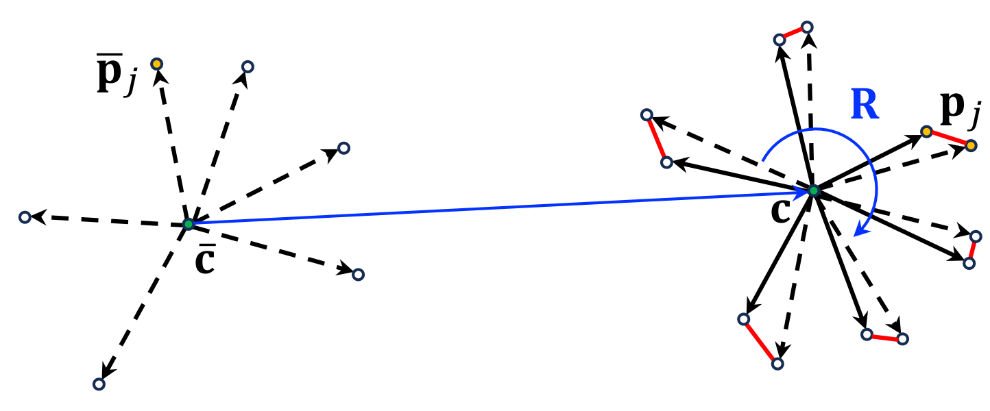
2.2. Least-Squares Estimation of Rigid Transformation

Least-squares estimation of rigid transformation between two sets of corresponding points is at the heart of our approach. It has been introduced in computer vision [8,9,10,11], and it is sometimes called the absolute orientation problem [12]. In computer graphics, this method has found application in meshless deformation, involving shape matching of vertices [13], and has been further extended to encompass shape matching with oriented particles [14]. Additionally, it has been employed in as-rigid-as-possible shape deformation with vertices [15] and extended to address oriented particles [16].

Given two sets of corresponding points, denoted by ${\overline{\mathbf{p}}}_j$ and ${\mathbf{p}}_j$, respectively, there exists a rigid transformation that optimally aligns two sets in a least-squares sense, as illustrated in Figure 1. This can be formulated as finding the optimal rotation matrix, $\mathbf{R}$, that minimizes

$$\sum w_j{\parallel \mathbf{R}({\overline{\mathbf{p}}}_j-\overline{\mathbf{c}})-({\mathbf{p}}_j-\mathbf{c})\parallel }^2,$$

(5)

where $w_j$ is a weight and $({\mathbf{p}}_j-\mathbf{c})$ and $({\overline{\mathbf{p}}}_j-\overline{\mathbf{c}})$ represent the relative positions of the points with respect to the weighted centers $\mathbf{c}$ and $\overline{\mathbf{c}}$, respectively. Here, the optimal translation is $(\mathbf{c}-\overline{\mathbf{c}})$.

The rotation matrix, $\mathbf{R}$, can be obtained through the polar decomposition of the covariance matrix [11]:

$$\mathbf{A}=\sum w_j({\mathbf{p}}_j-\mathbf{c}){({\overline{\mathbf{p}}}_j-\overline{\mathbf{c}})}^{\mathrm{T}}=\mathbf{R}\mathbf{S}.$$

(6)

If a point ${\mathbf{p}}_i$ needs to be fixed, the centers $\mathbf{c}$ and $\overline{\mathbf{c}}$ are replaced by ${\mathbf{p}}_i$ and ${\overline{\mathbf{p}}}_i$, respectively, as in the as-rigid-as-possible shape deformation approach [15,16]. We will apply this shape-matching technique to the 1-ring neighbors of each vertex, aligning them from texture space to world space.

3. Method

3.1. Problem

The objective of this paper is to develop an intuitive but rigorous method for computing an orthonormal tangent space denoted as ${\mathbf{T}}_i=[{\mathbf{t}}_i|{\mathbf{b}}_i\left|{\mathbf{n}}_i\right]$ at every vertex i of a triangular mesh provided with texture coordinates, as illustrated in Figure 2. The inclusion of the normal vector, ${\mathbf{n}}_i$, is optional. If ${\mathbf{n}}_i$ is not provided, it can be computed simultaneously with the tangent vector, ${\mathbf{t}}_i$, and the bitangent vector, ${\mathbf{b}}_i$ (see Section 3.2). Conversely, if ${\mathbf{n}}_i$ is supplied, the computation of ${\mathbf{t}}_i$ and ${\mathbf{b}}_i$ should conform to the direction defined by ${\mathbf{n}}_i$ (see Section 3.3). It is crucial to ensure that the vectors ${\mathbf{t}}_i$, ${\mathbf{b}}_i$, and ${\mathbf{n}}_i$ maintain orthogonality and unit length. This is essential for establishing a consistent local coordinate frame, known as TBN, at the vertex. Furthermore, the TBN frame should exhibit coherence with the frames of neighboring vertices within the mesh.

Texture mapping often introduces discontinuities where certain edges in a geometric model are duplicated in texture space, each with a different location. These discontinuities, referred to as seams, are illustrated in Figure 2 as magenta lines. Seams are inevitable in the texture mapping process, especially when applying a 2D texture to a closed surface mesh representing a solid object. To address seams, vertex duplication is necessary. The duplicated vertices have the same spatial position but distinct texture coordinates. This concept is similar to vertex duplication at a hard edge, which represents a sharp, distinct boundary or transition between adjacent faces. However, addressing vertex duplicates at a seam requires ensuring a smooth and coherent transition of the tangent space, unlike vertex duplicates at a hard edge. Failing to achieve this smoothness and coherence can result in visible boundaries where abrupt shading changes occur [2]. Initially, we handle vertices without duplication, followed by addressing seams (see Section 3.4).

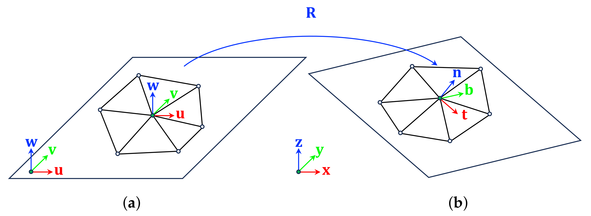
3.2. Solution Method for Unconstrained Normal Vectors

To produce coherent orthonormal tangent spaces across neighboring vertices, we adopt a least-squares estimation approach for optimal rotation between two sets of corresponding points. Let ${\mathcal{N}}_i$ represent the 1-ring neighborhood of a vertex, i, which consists of the vertices of the triangles sharing vertex i, as illustrated in Figure 3. We consider the vertices of ${\mathcal{N}}_i$ in both texture space and world space as two sets of corresponding points.

Without loss of generality, we embed texture space within world space by aligning the u-, v-, and w-axes of texture space with the x-, y-, and z-axes of world space, respectively. Here, the virtual w-axis is defined as the cross product of the u- and v-axes. Let ${\overline{\mathbf{p}}}_j=(u_j,v_j,0)$ represent the texture coordinates of vertex j, and ${\mathbf{p}}_j=(x_j,y_j,z_j)$ represent the corresponding world coordinates. We then seek the optimal rotation ${\mathbf{R}}_i$ that minimizes

$$\sum _{j\in {\mathcal{N}}_i}{w}_{ij}{\parallel {\mathbf{R}}_i({\overline{\mathbf{p}}}_j-{\overline{\mathbf{p}}}_i)-({\mathbf{p}}_j-{\mathbf{p}}_i)\parallel }^2,$$

(7)

where $w_{ij}=\frac{1}{2}(cot{\alpha }_{ij}+cot{\beta }_{ij})$ is the cotangent weight for an edge, $e_{ij}$, with the opposite angles ${\alpha }_{ij}$ and ${\beta }_{ij}$ [15,17]. This optimal rotation can be interpreted as a local space transformation. The rotation, ${\mathbf{R}}_i$, transforms the u-, v-, and w-axes of texture space into ${\mathbf{t}}_i$, ${\mathbf{b}}_i$, and ${\mathbf{n}}_i$, respectively, defining the tangent space at vertex i. The u-, v-, and w-axes are algebraically represented as $(1,0,0)$, $(0,1,0)$, and $(0,0,1)$ in the embedded world space. Consequently, the first, second, and third columns of ${\mathbf{R}}_i$ correspond to ${\mathbf{t}}_i$, ${\mathbf{b}}_i$, and ${\mathbf{n}}_i$, respectively. Therefore, the optimal rotation, ${\mathbf{R}}_i$, directly defines the tangent space: ${\mathbf{T}}_i=[{\mathbf{t}}_i|{\mathbf{b}}_i\left|{\mathbf{n}}_i\right]={\mathbf{R}}_i$. Note that ${\mathbf{t}}_i,{\mathbf{b}}_i$, and ${\mathbf{n}}_i$ are mutually orthogonal unit vectors because they constitute the three column vectors of the rotation matrix, ${\mathbf{R}}_i$.

The optimal rotation, ${\mathbf{R}}_i$, can be obtained using the polar decomposition of the covariance matrix:

$${\mathbf{A}}_i=\sum _{j\in {\mathcal{N}}_i}{w}_{ij}({\mathbf{p}}_j-{\mathbf{p}}_i){({\overline{\mathbf{p}}}_j-{\overline{\mathbf{p}}}_i)}^{\mathrm{T}}={\mathbf{R}}_i{\mathbf{S}}_i.$$

(8)

The third column of ${\mathbf{A}}_i$ is the $3\times 1$ zero vector because the third coordinate of every $({\overline{\mathbf{p}}}_j-{\overline{\mathbf{p}}}_i)$ is zero. This implies that the rank of ${\mathbf{A}}_i$ is 2. Nevertheless, the optimal rotation is unique because the rank is only one less than the dimension, as stated in [11].

To ensure robust computation of the polar decomposition, even with ${\mathbf{A}}_i$ of rank 2, we utilize singular value decomposition. In addition, for accurate computation of singular value decomposition we employ the Jacobi method provided in the Eigen library (eigen.tuxfamily.org). Let ${\mathbf{A}}_i={\mathbf{U}}_i{\Sigma }_i{\mathbf{V}}_i^{\mathrm{T}}$ be the singular value decomposition (${\mathbf{U}}_i{\mathbf{U}}_i^{\mathrm{T}}={\mathbf{V}}_i{\mathbf{V}}_i^{\mathrm{T}}=\mathbf{I}$ and ${\Sigma }_i=diag({\alpha }_i,{\beta }_i,0),{\alpha }_i\ge {\beta }_i$). Then, ${\mathbf{R}}_i={\mathbf{U}}_i{\mathbf{V}}_i^{\mathrm{T}}$. If $det\left({\mathbf{U}}_i\right)det\left({\mathbf{V}}_i\right)=-1$, it is essential to invert the sign of the third column of ${\mathbf{U}}_i$ (or ${\mathbf{V}}_i$) before computing ${\mathbf{R}}_i$. This inversion ensures that the resulting rotation matrix has a determinant of 1, making it a valid rotation matrix.

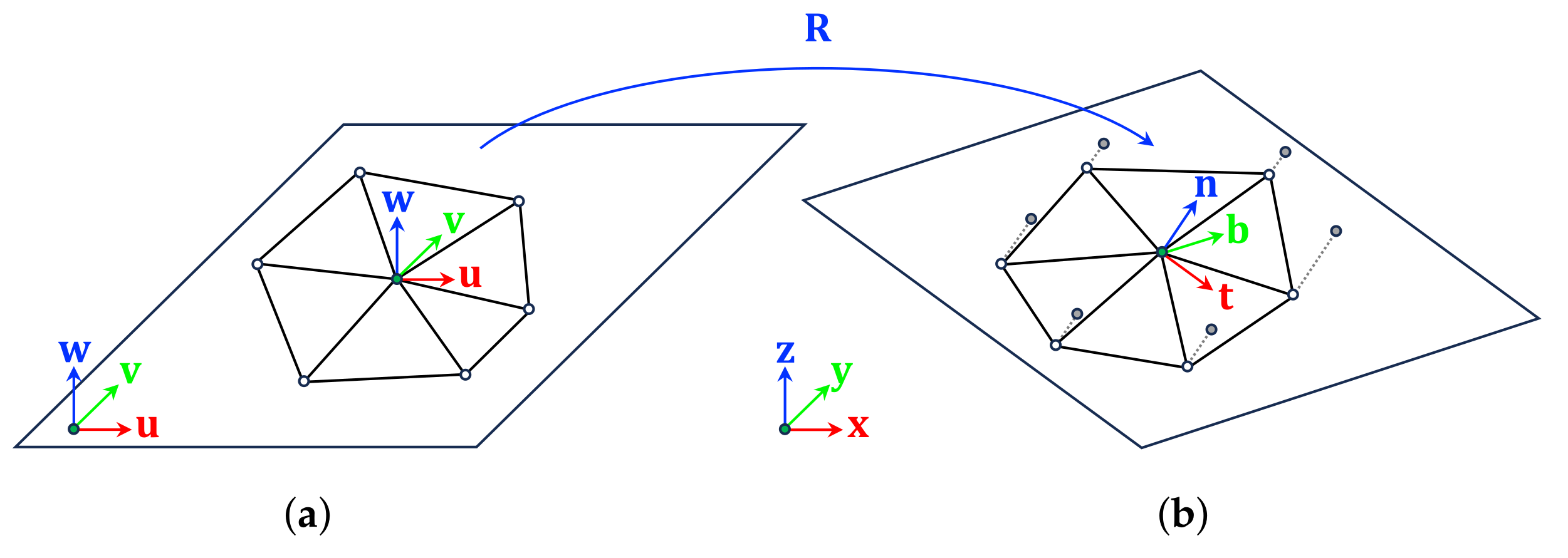
3.3. Solution Method for Constrained Normal Vectors

Certain triangular meshes are equipped with vertex-normal vectors and texture coordinates. However, computation of tangent space is still necessary in these cases. When the normal vector, ${\mathbf{n}}_i$, is provided, the third column of the optimal rotation matrix, ${\mathbf{R}}_i$, should be fixed to ${\mathbf{n}}_i$. Directly solving this constrained optimization can be challenging. Instead, we can rotate the relative positions $({\mathbf{p}}_j-{\mathbf{p}}_i)$ for all $j\in {\mathcal{N}}_i$ such that ${\mathbf{n}}_i$ aligns with the w-axis. This approach simplifies the task of finding the optimal 3D rotation to determine the optimal 2D rotation about the w-axis. After this rotation, $({\mathbf{p}}_j-{\mathbf{p}}_i)$ can be projected onto the $uv$-plane, as their distances along the w-axis remain unchanged. Consequently, the problem is reduced to finding the optimal 2D rotation between two sets of vertex positions on the texture plane.

Alternatively, we can directly deal with the projection of $({\mathbf{p}}_j-{\mathbf{p}}_i)$ onto the plane perpendicular to ${\mathbf{n}}_i$ in world space, as depicted in Figure 4. This involves calculating the vector rejection of $({\mathbf{p}}_j-{\mathbf{p}}_i)$ from ${\mathbf{n}}_i$. The vector rejection of $\mathbf{a}$ from $\mathbf{b}$ is defined as ${\mathbf{a}}_{\perp \mathbf{b}}=(\mathbf{a}-{\mathbf{a}}_{\parallel \mathbf{b}})$, where ${\mathbf{a}}_{\parallel \mathbf{b}}$ is the vector projection of $\mathbf{a}$ onto $\mathbf{b}$, calculated as $(\mathbf{a}·\frac{\mathbf{b}}{\parallel \mathbf{b}\parallel })\frac{\mathbf{b}}{\parallel \mathbf{b}\parallel }$. The problem is then reduced to finding the optimal rotation between the two sets of corresponding vectors $({\overline{\mathbf{p}}}_j-{\overline{\mathbf{p}}}_i)$ and ${({\mathbf{p}}_j-{\mathbf{p}}_i)}_{\perp {\mathbf{n}}_i}$ for all $j\in {\mathcal{N}}_i$. This can be formulated as finding the rotation matrix, ${\mathbf{R}}_i$, that minimizes

$$\sum _{j\in {\mathcal{N}}_i}{w}_{ij}{\parallel {\mathbf{R}}_i({\overline{\mathbf{p}}}_j-{\overline{\mathbf{p}}}_i)-{({\mathbf{p}}_j-{\mathbf{p}}_i)}_{\perp {\mathbf{n}}_i}\parallel }^2.$$

(9)

Then, ${\mathbf{R}}_i$ can be obtained with the polar decomposition of the covariance matrix:

$${\mathbf{A}}_i=\sum _{j\in {\mathcal{N}}_i}{w}_{ij}{({\mathbf{p}}_j-{\mathbf{p}}_i)}_{\perp {\mathbf{n}}_i}{({\overline{\mathbf{p}}}_j-{\overline{\mathbf{p}}}_i)}^{\mathrm{T}}={\mathbf{R}}_i{\mathbf{S}}_i.$$

(10)

Here, the third column of ${\mathbf{R}}_i$ aligns with ${\mathbf{n}}_i$ because any out-of-plane rotation increases the distances between the two sets of vectors. This method is preferable to the first method, as it is consistent with the approach for unconstrained normal vectors, with the addition of vector rejection.

By utilizing ${({\mathbf{p}}_j-{\mathbf{p}}_i)}_{\perp {\mathbf{n}}_i}=(\mathbf{I}-{\mathbf{n}}_i{\mathbf{n}}_i^{\mathrm{T}})({\mathbf{p}}_j-{\mathbf{p}}_i)$, Equation (10) can be further reformulated as follows:

$${\mathbf{A}}_i=(\mathbf{I}-{\mathbf{n}}_i{\mathbf{n}}_i^{\mathrm{T}})\sum _{j\in {\mathcal{N}}_i}{w}_{ij}({\mathbf{p}}_j-{\mathbf{p}}_i){({\overline{\mathbf{p}}}_j-{\overline{\mathbf{p}}}_i)}^{\mathrm{T}}={\mathbf{R}}_i{\mathbf{S}}_i.$$

(11)

This equation is quite similar to Equation (8), but it involves projecting the covariance matrix itself onto the plane perpendicular to ${\mathbf{n}}_i$ before decomposing it into the rotation matrix and the stretch matrix. It is worth noting that computing the tangent space using Equation (11) is slightly more computationally efficient compared to Equation (10).

3.4. Texture Space Alignment for Seams

Vertex duplicates on seams are individually indexed, leading to the independent computation of their tangent spaces without special consideration. To address this issue, it is necessary to identify these duplicated vertices and compute their tangent spaces while considering their neighboring vertices collectively. This approach is similar to that described in [2], where vertex duplicates are identified and their tangent vectors are averaged and set equal to each other if they align in similar directions. However, our method differs from [2] in that we apply a rigid transformation in texture space to each set of triangles adjacent to each duplicated vertex, as illustrated in Figure 5. This transformation aims to align both sides of every seam as closely as possible. The vertices aligned in this manner within texture space are then used to estimate the optimal rotation for the corresponding vertices in world space. Our approach is motivated by the fact that seams were initially placed only at their current location during the texture unwrapping process, but they could potentially have been relocated elsewhere through neighboring triangles. Therefore, when computing the tangent space, neighboring triangles should be considered across seams.

Consider a vertex, i, with n seams, as depicted in Figure 5, where $n=3$ for simplicity. The duplicated vertices are labeled as $i_j$ for $j\in [1,n]$, with $i_1=i$ without loss of generality. For each seam, j, matching edges are identified as ordered pairs $(i_j,k_j)$ and $(i_{j+1},l_{j+1})$, utilizing circular indexing for j. The triangles adjacent to vertex $i_j$ for $j\in [2,n]$ undergo a rigid transformation that translates vertex $i_j$ to coincide with vertex $i_1$. This transformation also rotates the two seam edges by ${\overline{\mathbf{R}}}_{i_j}$ in texture space to optimally align them with their matching edges in a least-squares sense. The notation $\overline{\mathbf{R}}$ is used to distinguish the rotation in texture space from the rotation for the tangent space. Thus, the optimal texture space alignment can be formulated as finding the rotation matrices, ${\overline{\mathbf{R}}}_{i_j}$, for all $j\in [2,n]$ that minimize

$$\sum _{j=1}^n{\parallel {\overline{\mathbf{R}}}_{i_j}({\overline{\mathbf{p}}}_{k_j}-{\overline{\mathbf{p}}}_{i_j})-{\overline{\mathbf{R}}}_{i_{j+1}}({\overline{\mathbf{p}}}_{l_{j+1}}-{\overline{\mathbf{p}}}_{i_{j+1}})\parallel }^2,$$

(12)

where ${\overline{\mathbf{R}}}_{i_1}$ is set to $\mathbf{I}$ for notational convenience.

Solving the optimal rotations, ${\overline{\mathbf{R}}}_{i_j}$s, simultaneously can be challenging. Instead, we adopt an iterative approach to optimize ${\overline{\mathbf{R}}}_{i_j}$ for $j\in [2,n]$, assuming that only ${\overline{\mathbf{R}}}_{i_j}$ can change while the others are fixed. The optimal rotation ${\overline{\mathbf{R}}}_{i_j}$ is then obtained using the polar decomposition of the covariance matrix:

$${\overline{\mathbf{A}}}_{i_j}={\overline{\mathbf{R}}}_{i_{j+1}}({\overline{\mathbf{p}}}_{l_{j+1}}-{\overline{\mathbf{p}}}_{i_{j+1}}){({\overline{\mathbf{p}}}_{k_j}-{\overline{\mathbf{p}}}_{i_j})}^{\mathrm{T}}+{\overline{\mathbf{R}}}_{i_{j-1}}({\overline{\mathbf{p}}}_{k_{j-1}}-{\overline{\mathbf{p}}}_{i_{j-1}}){({\overline{\mathbf{p}}}_{l_j}-{\overline{\mathbf{p}}}_{i_j})}^{\mathrm{T}}={\overline{\mathbf{R}}}_{i_j}{\overline{\mathbf{S}}}_{i_j}.$$

(13)

A good initial guess is crucial in reducing the number of iterations. We sequentially align edge $(i_j,l_j)$ with edge $(i_{j-1},k_{j-1})$ by rotating the triangles adjacent to vertex $i_j$ and set the rotation as an initial guess of ${\overline{\mathbf{R}}}_{i_j}$ for $j\in [2,n]$. Starting from these initial guesses, iterative optimization is performed until there are no significant changes in ${\overline{\mathbf{R}}}_{i_j}$s.

3.5. Incorporation of Texture Space Alignment

Now, ${\overline{\mathbf{R}}}_{i_j}$ can be incorporated into Equations (7)–(11). For example, Equation (8) is adapted to obtain the rotation matrix, ${\mathbf{R}}_i$, as follows:

$${\mathbf{A}}_i=\sum _{j=1}^n\sum _{k\in {\mathcal{N}}_{i_j}}{w}_{ik}({\mathbf{p}}_k-{\mathbf{p}}_i){\left[{\overline{\mathbf{R}}}_{i_j}({\overline{\mathbf{p}}}_k-{\overline{\mathbf{p}}}_{i_j})\right]}^{\mathrm{T}}={\mathbf{R}}_i{\mathbf{S}}_i$$

(14)

where ${\mathbf{A}}_{i_1}={\mathbf{A}}_i$, $w_{i_{j}k}=w_{ik}$, and ${\mathbf{p}}_{i_j}={\mathbf{p}}_i$ were employed. When vertex i has no duplicates, Equation (14) becomes exactly the same as Equation (8) because ${\overline{\mathbf{R}}}_{i_1}=\mathbf{I}$.

${\mathbf{A}}_{i_j}$ for $j\in [2,n]$ need not be computed from scratch to obtain ${\mathbf{R}}_{i_j}$. Instead, we can directly obtain ${\mathbf{R}}_{i_j}$ from ${\mathbf{R}}_i$ by

$${\mathbf{R}}_{i_j}={\mathbf{R}}_i{\overline{\mathbf{R}}}_{i_j}.$$

(15)

This simplification arises because the triangles sharing vertex $i_j$ undergo ${\overline{\mathbf{R}}}_{i_j}$ in texture space to optimally align their two seam edges with the matching edges. Subsequently, all vertices of the triangles sharing the duplicates undergo ${\mathbf{R}}_i$ for optimal matching with their corresponding vertices in world space. Equation (15) highlights that each duplicate has a distinct tangent space, differing from the tangent spaces of other duplicates by the amount of the differences in optimal alignment in texture space, as illustrated in Figure 2c.

Equation (15) can also be derived algebraically. To compute ${\mathbf{A}}_{i_l}$ as in Equation (14), for a certain vertex $i_l$, we need to rewrite the rotation matrix, ${\mathbf{R}}_{i_j}$, with respect to vertex $i_l$, resulting in ${\mathbf{R}}_{i_l}^{\mathrm{T}}{\mathbf{R}}_{i_j}$. Then, the covariance matrix is written as

$${\mathbf{A}}_{i_l}=\sum _{j=1}^n\sum _{k\in {\mathcal{N}}_{i_j}}{w}_{ik}({\mathbf{p}}_k-{\mathbf{p}}_i){\left[{\overline{\mathbf{R}}}_{i_l}^{\mathrm{T}}{\overline{\mathbf{R}}}_{i_j}({\overline{\mathbf{p}}}_k-{\overline{\mathbf{p}}}_{i_j})\right]}^{\mathrm{T}}={\mathbf{A}}_i{\overline{\mathbf{R}}}_{i_l}.$$

(16)

Utilizing ${\mathbf{A}}_i={\mathbf{R}}_i{\mathbf{S}}_i$ given in Equation (14), we obtain

$${\mathbf{A}}_{i_l}={\mathbf{R}}_i{\mathbf{S}}_i{\overline{\mathbf{R}}}_{i_l}={\mathbf{R}}_i\left({\overline{\mathbf{R}}}_{i_l}{\overline{\mathbf{R}}}_{i_l}^{\mathrm{T}}\right){\mathbf{S}}_i{\overline{\mathbf{R}}}_{i_l}=\left({\mathbf{R}}_i{\overline{\mathbf{R}}}_{i_l}\right)\left({\overline{\mathbf{R}}}_{i_l}^{\mathrm{T}}{\mathbf{S}}_i{\overline{\mathbf{R}}}_{i_l}\right)={\mathbf{R}}_{i_l}{\mathbf{S}}_{i_l}.$$

(17)

From this result, we observe that ${\mathbf{R}}_{i_l}={\mathbf{R}}_i{\overline{\mathbf{R}}}_{i_l}$. Replacing index l with j gives the tangent space of vertex $i_j$, ${\mathbf{R}}_{i_j}={\mathbf{R}}_i{\overline{\mathbf{R}}}_{i_j}$, which matches the formula given in Equation (15).

3.6. Application of Texture Space Alignment

Furthermore, the optimal alignment in texture space can be utilized to average tangent spaces in the previous methods [2,3,5]. To do this, we first reformulate Equation (3) by employing the texture coordinates ${\overline{\mathbf{p}}}_0=(u_0,v_0,0)$, ${\overline{\mathbf{p}}}_1=(u_1,v_1,0)$, and ${\overline{\mathbf{p}}}_2=(u_2,v_2,0)$ of a triangle and the w-axis $\mathbf{w}=(0,0,1)$ as follows:

$$\left[({\mathbf{p}}_1-{\mathbf{p}}_0)\left|({\mathbf{p}}_2-{\mathbf{p}}_0)\right|\mathbf{n}\right]=\left[\mathbf{t}\left|\mathbf{b}\right|\mathbf{n}\right]\left[({\overline{\mathbf{p}}}_1-{\overline{\mathbf{p}}}_0)\left|({\overline{\mathbf{p}}}_2-{\overline{\mathbf{p}}}_0)\right|\mathbf{w}\right].$$

(18)

The tangent space of the triangle is then obtained by

$$\left[\mathbf{t}\left|\mathbf{b}\right|\mathbf{n}\right]=\left[({\mathbf{p}}_1-{\mathbf{p}}_0)\left|({\mathbf{p}}_2-{\mathbf{p}}_0)\right|\mathbf{n}\right]{\left[({\overline{\mathbf{p}}}_1-{\overline{\mathbf{p}}}_0)\left|({\overline{\mathbf{p}}}_2-{\overline{\mathbf{p}}}_0)\right|\mathbf{w}\right]}^{-1},$$

(19)

which corresponds to Equation (4).

If one of the vertices of the triangle is a duplicated vertex $i_j$ of vertex i on a seam, the optimal alignment, ${\overline{\mathbf{R}}}_{i_j}$, is employed to obtain the tangent space of the triangle aligned with respect to vertex i:

$$\left[{\mathbf{t}}_A\left|{\mathbf{b}}_A\right|\mathbf{n}\right]=\left[({\mathbf{p}}_1-{\mathbf{p}}_0)\left|({\mathbf{p}}_2-{\mathbf{p}}_0)\right|\mathbf{n}\right]{\left({\overline{\mathbf{R}}}_{i_j}\left[({\overline{\mathbf{p}}}_1-{\overline{\mathbf{p}}}_0)\left|({\overline{\mathbf{p}}}_2-{\overline{\mathbf{p}}}_0)\right|\mathbf{w}\right]\right)}^{-1}.$$

(20)

This is equivalent to computing the tangent space of the triangle using the aligned texture coordinates, as in Figure 5b, instead of the original coordinates, as in Figure 5a. The above equation can be further written as

$$\left[{\mathbf{t}}_A\left|{\mathbf{b}}_A\right|\mathbf{n}\right]=\left[\mathbf{t}\left|\mathbf{b}\right|\mathbf{n}\right]{\overline{\mathbf{R}}}_{i_j}^{\mathrm{T}}.$$

(21)

Finally, the tangent space $\left[{\mathbf{t}}_i\right|{\mathbf{b}}_i\left|{\mathbf{n}}_i\right]$ of vertex i is computed by averaging all the tangent spaces of the triangles aligned in this manner. The tangent space of the duplicated vertex $i_j$ can also be directly obtained from $\left[{\mathbf{t}}_i\right|{\mathbf{b}}_i\left|{\mathbf{n}}_i\right]$ as follows:

$$\left[{\mathbf{t}}_{i_j}\left|{\mathbf{b}}_{i_j}\right|{\mathbf{n}}_{i_j}\right]=\left[{\mathbf{t}}_i\left|{\mathbf{b}}_i\right|{\mathbf{n}}_i\right]{\overline{\mathbf{R}}}_{i_j}.$$

(22)

The derivation for the above simplification is similar to that employed for Equation (15).

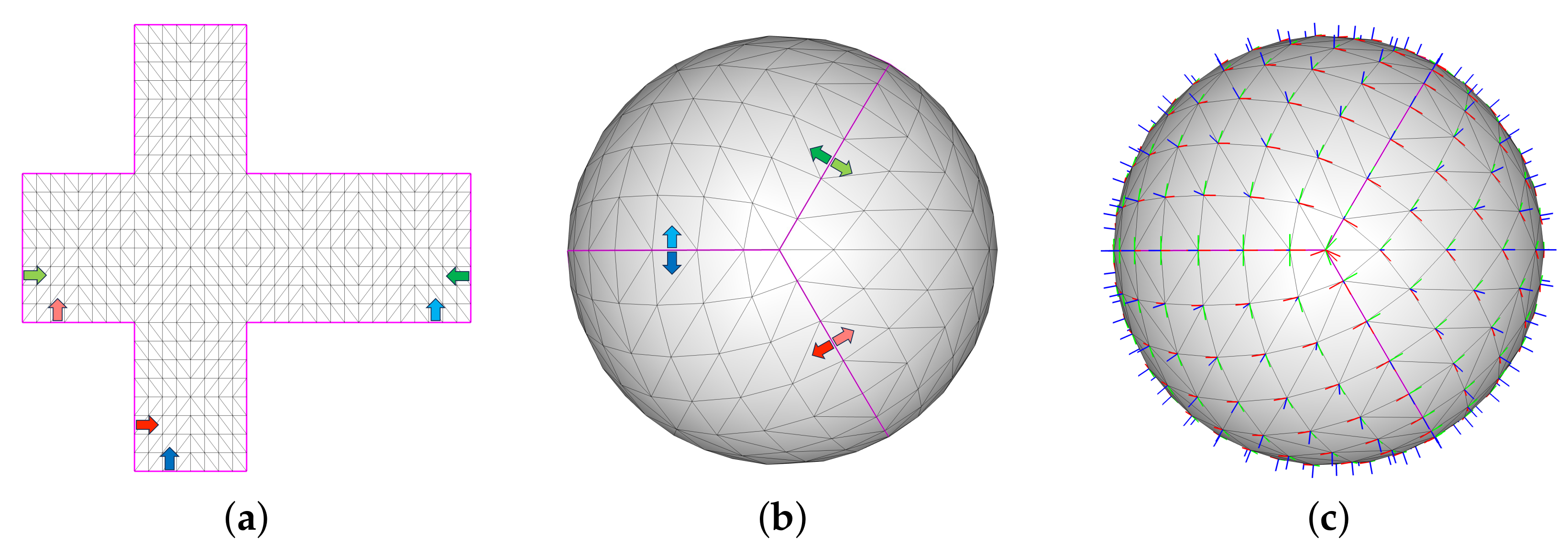
4. Experimental Results

We first conducted an experiment on a triangular mesh of a sphere model provided with vertex-normal vectors, as shown in Figure 2. The tangent spaces computed with our method exhibit coherence with the neighboring tangent spaces, even at the seams, owing to the texture space alignment. To further demonstrate the effectiveness of the texture space alignment for seams, we applied our method, the linear method [2,5], and Mikkelsen’s method [3] to the sphere model, both with and without the texture space alignment. Figure 6 shows the tangent spaces obtained for the six cases. It can be observed that the texture space alignment is effective in ensuring smooth transitions across seams, not only in our method but also in the linear method and Mikkelsen’s method.

Now, we analyze the orthonormality errors in the tangent spaces obtained with the previous methods. The tangent space obtained at a vertex using the linear method [2,5] is denoted as ${\mathbf{T}}_l=[{\mathbf{t}}_l|{\mathbf{b}}_l\left|{\mathbf{n}}_l\right]$. As detailed in Section 2.1, ${\mathbf{T}}_l$ should undergo the Gram–Schmidt orthonormalization process, which adjusts the tangent and bitangent vectors. However, for a thorough examination of inherent orthonormality errors, we omit the Gram–Schmidt process and exclusively utilize vector normalization, which is a straightforward procedure necessary to compensate for the scale difference between the tangent space and the world space. The tangent space obtained with Mikkelsen’s method [3] is represented as ${\mathbf{T}}_m=[{\mathbf{t}}_m|{\mathbf{b}}_m\left|{\mathbf{n}}_m\right]$.

We analyzed the orthonormality errors in a triangular mesh of a cow model, which is provided with vertex-normal vectors. The orthonormality error in ${\mathbf{T}}_l$ of the linear method is measured by the metric $\parallel \mathbf{I}-{\mathbf{T}}_l^{\mathrm{T}}{\mathbf{T}}_l{\parallel }_{\mathrm{F}}$, where ${\parallel ·\parallel }_{\mathrm{F}}$ represents the Frobenius norm of a matrix. Figure 7a visualizes this orthonormality error at every vertex. The first column visualizes the errors in the surface, the second column in the vertices, and the third column in texture space. The last column shows the histogram of the errors on a logarithmic scale. We can observe that there are large errors in sharp features. Figure 7b shows the orthonormality errors in ${\mathbf{T}}_m$ of Mikkelsen’s method. The errors are smaller than those in the linear method because the tangent vectors and the bitangent vectors are orthogonal to the normal vectors.

Then, we compared the tangent spaces obtained with the previous methods to the orthonormal tangent spaces ${\mathbf{T}}_s=[{\mathbf{t}}_s|{\mathbf{b}}_s\left|{\mathbf{n}}_s\right]$ obtained with our shape-matching-based method. Figure 7c,d shows the differences of ${\mathbf{T}}_l$ and ${\mathbf{T}}_m$ compared to ${\mathbf{T}}_s$. The differences are measured by $\parallel {\mathbf{T}}_l-{\mathbf{T}}_s{\parallel }_{\mathrm{F}}$ and $\parallel {\mathbf{T}}_m-{\mathbf{T}}_s{\parallel }_{\mathrm{F}}$. We can observe that the differences are also large where the orthonormality errors are large. Figure 8 shows the close-up view of the horn with the red, green, and blue axes corresponding to the tangent, bitangent, and normal vectors. The bright, thick axes represent the orthonormal tangent spaces obtained with our method, while the dark, thin ones represent those with either the linear method or Mikkelsen’s method. The three axes at the tip of the right horn has a large error and are far from orthogonal.

The experiments were conducted on a MacBook Pro laptop equipped with an Apple M2 Max CPU, utilizing only a single core and thread to measure CPU time for computation. Reading an ASCII file containing a cow model with 2904 vertices, 8706 edges, 5804 faces, 3195 texture coordinates, and 292 seam edges took approximately 8.10 ms. Texture space alignment required approximately 0.32 ms, and tangent space computation with our method took approximately 1.01 ms. Tangent space computation using both the linear method and Mikkelsen’s method each took approximately 0.34 ms. Our method demanded more computation than the previous methods due to the heavier workload of the polar decomposition of the covariance matrix employed in our method, compared to the matrix inversion used in the previous method.

The next experiment is for the sphere model, where the tangent spaces of adjacent triangles and vertices are expected to be very similar due to the inherent geometry of a sphere. Figure 9 shows the result of this experiment. Although the orthonormality errors were smaller compared to those in the cow model, they remained non-negligible. The first column displays a close-up view, featuring the bright, thick axes representing the tangent spaces obtained with our method, alongside the dark, thin axes obtained with either the linear method or Mikkelsen’s method. Mikkelsen’s method exhibits lower orthonormality errors than the linear method.

For a triangular mesh without vertex-normal vectors, our shape-matching method can generate normal vectors in addition to tangent and bitangent vectors. In the case of a smooth triangular mesh, the generated normal vectors are satisfactory, as illustrated in the sphere model shown in Figure 10a. The normal vectors provided with the mesh were discarded, and new ones were computed using both our shape-matching method and the linear method. The differences $\parallel {\mathbf{n}}_s-{\mathbf{n}}_l\parallel$ are overlaid onto the surface. However, normal vectors for sharp features are less satisfactory, as demonstrated in Figure 10b. It is important to note that the normal vector depends solely on the underlying geometry and is not influenced by the texture map. Consequently, we recommend using the average of face normals, as was done in the linear method, to compute the normal vectors. Our method can then be applied to obtain orthonormal tangent spaces for the constrained normal vectors.

5. Conclusions

In this paper, we have developed an intuitive yet rigorous method for computing per-vertex tangent spaces in a triangular mesh with texture coordinates. Our method utilizes least-squares estimation of rigid transformation to align the 1-ring neighbor vertices of a vertex in texture space with the corresponding vertices in world space. One notable advantage of our method is its inherent generation of orthonormal tangent spaces, eliminating the need for the intricate operations, such as averaging and orthonormalization, required in the previous methods [2,3,5]. In addition, we have introduced a novel approach for aligning texture space triangles to address seams inherent in texture mapping to a closed surface mesh. This approach also employs least-squares estimation of rigid transformations in texture space to align both sides of every seam as closely as possible. To our knowledge, texture space alignment for seams has been introduced for the first time in this paper. Furthermore, it can be used to average tangent spaces in the previous methods. Currently, our method deals with triangular meshes only, but it can potentially be extended to polygonal meshes by modifying the weights for the least-squares estimation process.

References

1. Kilgard, M.J. A Practical and Robust Bump-mapping Technique for Today’s GPUs. In Proceedings of the Game Developers Conference Course: Advanced OpenGL Game Development, New Orleans, LA, USA, 23–28 July 2000. [Google Scholar]
2. Lengyel, E. Foundations of Game Engine Development, Volume 2: Rendering; Terathon Software LLC: Lincoln, CA, USA, 2019. [Google Scholar]
3. Mikkelsen, M. Simulation of Wrinkled Surfaces Revisited. Master’s Thesis, Department of Computer Science at the University of Copenhagen, Copenhagen, Denmark, 2008. [Google Scholar]
4. De Vries, J. Learn OpenGL: Learn Modern OpenGL Graphics Programming in a Step-by-Step Fashion; Kendall & Welling: Kendall, FL, USA, 2020. [Google Scholar]
5. Lengyel, E. Computing Tangent Space Basis Vectors for an Arbitrary Mesh; Technical Report; Terathon Software 3D Graphics Library: Lincoln, CA, USA, 2001; Available online: http://www.terathon.com/code/tangent.html (accessed on 20 March 2024).
6. Lengyel, E. Mathematics for 3D Game Programming and Computer Graphics; Cengage Learning: Boston, MA, USA, 2011. [Google Scholar]
7. Mittring, M. Shader X4 Advanced Rendering Techniques; Chapter Triangle Mesh Tangent Space Calculation; Charles River Media: Hingham, MA, USA, 2005. [Google Scholar]
8. Huang, T.S.; Blostein, S.D.; Margerum, E.A. Least-squares estimation of motion parameters from 3-D point correspondences. In Proceedings of the IEEE Conference on Computer Vision and Pattern Recognition, Miami Beach, FL, USA, 22–26 June 1986; pp. 24–26. [Google Scholar]
9. Arun, K.S.; Huang, T.S.; Blostein, S.D. Least-squares fitting of two 3-D point sets. IEEE Trans. Pattern Anal. Mach. Intell. 1987, 9, 698–700. [Google Scholar] [CrossRef] [PubMed]
10. Horn, B.K.P. Closed-form solution of absolute orientation using orthonormal matrices. J. Opt. Soc. Am. 1987, 5, 1127–1135. [Google Scholar] [CrossRef]
11. Umeyama, S. Least-squares estimation of transformation parameters between two point patterns. IEEE Trans. Pattern Anal. Mach. Intell. 1991, 13, 376–380. [Google Scholar] [CrossRef]
12. Horn, B.K.P. Closed-form solution of absolute orientation using unit quaternions. J. Opt. Soc. Am. 1987, 4, 629–642. [Google Scholar] [CrossRef]
13. Müller, M.; Heidelberger, B.; Teschner, M.; Gross, M. Meshless Deformations Based on Shape Matching. ACM Trans. Graph. 2005, 24, 471–478. [Google Scholar] [CrossRef]
14. Müller, M.; Chentanez, N. Solid Simulation with Oriented Particles. ACM Trans. Graph. 2011, 30, 92. [Google Scholar] [CrossRef]
15. Sorkine, O.; Alexa, M. As-rigid-as-possible surface modeling. In Proceedings of the Eurographics Symposium on Geometry Processing, Barcelona, Spain, 4–6 July 2007; pp. 109–116. [Google Scholar]
16. Choi, M.G.; Lee, J. As-Rigid-As-Possible Solid Simulation with Oriented Particles. Comput. Graph. 2018, 70, 1–7. [Google Scholar] [CrossRef]
17. Pinkall, U.; Polthier, K. Computing discrete minimal surfaces and their conjugates. Exp. Math. 1993, 2, 15–36. [Google Scholar] [CrossRef]
Figure 1. Least-squares estimation of rigid transformation between two sets of corresponding points.
Applsci 14 02834 g001
Figure 2. Seams are represented as magenta lines in texture space and world space. The block arrows illustrate directions near the seam edges. The red, green, and blue axes represent the tangent, bitangent, and normal vectors of the tangent spaces. (a) Texture space; (b) World space; (c) Tangent space.
Applsci 14 02834 g002
Figure 3. Least-squares estimation of a rigid transformation that optimally aligns the positions of the 1-ring neighbors of a vertex in texture space with their corresponding positions in world space. (a) Texture space; (b) World space.
Applsci 14 02834 g003
Figure 4. Least-squares estimation for a constrained normal vector. The 1-ring neighbors are projected onto the plane perpendicular to the normal vector before computing the tangent space. (a) Texture space; (b) World space.
Applsci 14 02834 g004
Figure 5. Optimal alignment for seam edges. The triangles adjacent to the duplicated vertices are optimally aligned in texture space before computing the tangent space. (a) Texture space; (b) Aligned in texture space; (c) World space.
Applsci 14 02834 g005
Figure 6. The tangent space alignment for seams was employed in the top row but not in the bottom. (a) Our method; (b) The linear method; (c) Mikkelsen’s method.
Applsci 14 02834 g006
Figure 7. A triangular mesh of a cow model equipped with vertex-normal vectors. The first and second rows show the orthonormality errors in the tangent spaces T l and T m obtained with the linear method and Mikkelsen’s method, respectively. The third and fourth rows show the differences of T l and T m compared to T s obtained with our method. The error and differences are overlaid onto the surface in the first column, onto the vertices in the second column, and onto texture space in the third column. The last column shows the histogram on a logarithmic scale. (a) Orthonormality error I T l T T l F of the linear method; (b) Orthonormality error I T m T T m F of Mikkelsen’s method; (c) Difference T l T s F between the linear method and our method; (d) Difference T m T s F between Mikkelsen’s method and our method.
Applsci 14 02834 g007
Figure 8. Close-up view of the right horn of a cow model. The bright, thick RGB axes represent the tangent spaces obtained with our method, while the dark, thin ones represent those with either (a) the linear method or (b) Mikkelsen’s method.
Applsci 14 02834 g008
Figure 9. Orthonormality errors in a triangular mesh of a sphere model. (a) Orthonormality error I T l T T l F of the linear method; (b) Orthonormality error I T m T T m F of Mikkelsen’s method.
Applsci 14 02834 g009
Figure 10. Differences of normal vectors obtained by our method and the linear method. (a) Differences and histogram in a sphere model; (b) Differences and histogram in a cow model.
Applsci 14 02834 g010
Disclaimer/Publisher’s Note: The statements, opinions and data contained in all publications are solely those of the individual author(s) and contributor(s) and not of MDPI and/or the editor(s). MDPI and/or the editor(s) disclaim responsibility for any injury to people or property resulting from any ideas, methods, instructions or products referred to in the content.