Abstract
Chlorophyll-a (chl-a) serves as a key indicator in water quality and harmful algal blooms (HABs) research. While satellite ocean color data have greatly advanced chl-a research and HABs monitoring, missing data caused by cloud cover and other factors limit the spatiotemporal continuity and the utility of remote sensing data products. The Data Interpolating Empirical Orthogonal Function (DINEOF) method, widely used to reconstruct missing values in remote sensing datasets, is open to improvement in terms of computational accuracy and efficiency. We propose an improved method called Concentration-Stratified DINEOF (CS-DINEOF), which uses a coordinate–value correlative data division strategy to stratify the study area into several subregions based on annual average chl-a concentration. The proposed method clusters data points with similar spatiotemporal patterns, allowing for more targeted and effective reconstruction in each sub-dataset. The feasibility and advantage of the proposed method are tested and evaluated in the experiments of chl-a data reconstruction in the water of the Bohai Sea. Compared with the ordinary DINEOF method, the CS-DINEOF method improves the reconstruction accuracy, with an average Root Mean Square Error (RMSE) reduction of 0.0281 mg/m3, and saves computational time by 228.9%. Furthermore, the gap-free images generated from CS-DINEOF are able to illustrate small variations and details of the chl-a distribution in local areas. We can conclude that the proposed CS-DINEOF method is superior in providing significant insights for water quality and HABs studies in the Bohai Sea region.
1. Introduction
Harmful algal blooms (HABs) represent a deleterious ecological phenomenon stemming from the explosive proliferation of phytoplankton or bacteria in marine or brackish waters, which disrupt the delicate balance of ecosystems, negatively affect fisheries, and release toxic substances harmful to human health [1,2,3]. Over the past 30 years, HAB events have shown a significant increase in frequency, scale, and geographical distribution, evolving into a worldwide ecological problem [4]. Therefore, the monitoring of HABs has been a topic of concern for marine environmental scientists in the past several decades [5].
Chlorophyll-a (chl-a) serves as the main pigment of phytoplankton, and chl-a concentration is commonly adopted to characterize the diversity of phytoplankton and algae species [6]. Huot et al. [7] compared seven indicators of phytoplankton biomass and concluded that chl-a concentration can provide the most appropriate estimate of primary productivity. Consequently, chl-a has been regarded as a key indicator in HABs research and the detection of water nutrient levels [8]. In the fields of marine environment and water quality studies, chl-a concentration is defined as a proxy for phytoplankton concentration in surface waters [9,10]. Research on the chl-a concentration in seawater can be conducive to obtaining timely insights into algae progression and marine ecological status, and this provides early warnings for HABs events.
Traditional approaches of chl-a estimation involve field observation through on-site sensors and laboratory analysis of collected water samples, which are limited by their high-cost, time-consuming, and labor-intensive nature; therefore, they are unsuitable for large spatiotemporal scales [11,12]. Instead, satellite remote sensing technology, with its enhanced spatiotemporal coverage, has greatly advanced our comprehension of near-surface ocean phenomena and played an important role in supporting the monitoring of aquatic-related processes, especially HABs [13,14]. Therefore, a large amount of work based on remote sensing products has been conducted to explore chl-a, the important water quality variable, and carry out research on concentration inversion algorithms [15,16,17,18,19], environmental factors influencing mechanisms [20,21], trend prediction [4,22,23], and other aspects to assist HABs monitoring and prevention.
Achieving the large-scale, long-duration monitoring of chl-a concentration requires regularly collected and continuous data series [24]. However, challenges arise in ocean remote sensing data and their inversion products in the form of poor data quality and missing data due to factors such as cloud cover [25,26,27], solar glare pollution [28], and sensor faults. These issues significantly compromise the spatial and temporal continuity as well as the utility of data products [29]. To address these challenges, research has been conducted on techniques for data reconstruction. Conventional methods mainly include Optimal Interpolation (OI) [30], Singular Spectrum Analysis (SSA) [31], Expectation Maximization (EM) [32], and certain distance-based approaches such as Inverse Distance Weighting (IDW) [33] and Kriging [34,35]. In the field of remote sensing data applications, Data Interpolating Empirical Orthogonal Function (DINEOF) [36,37] is acknowledged as a robust technique [38]. Based on Empirical Orthogonal Functions (EOFs), the DINEOF method utilizes the inherent spatiotemporal consistency of the data, rather than relying on additional prior information, to derive values at missing locations. With the increasing availability and utilization of marine remote sensing data, the DINEOF method has been successfully employed in the reconstruction of missing data from various marine variables, such as sea surface temperature [39,40], salinity [41], and chl-a [42,43,44].
The performance of the DINEOF method can be heavily impacted by the characteristics of the research variable, region, and input dataset [44]. Therefore, specific improved reconstruction strategies are required in real-world applications. Wang and Liu [45] enhanced the DINEOF approach by introducing a depth-based dataset division strategy and an novel outlier detection process, yielding improved overall performance for gap filling. Ping et al. [46] presented an improved algorithm I-DINEOF, partitioning the initial dataset into multiple smaller matrices and reconstructing each matrix with the most appropriate EOF, thereby mitigating the sensitivity of the ordinary DINEOF to missing data. Furthermore, another improved algorithm, VE-DINEOF, was proposed [47], which optimized the ordinary DINEOF workflow by determining the optimal EOF for each iteration independently, resulting in a higher reconstruction accuracy and efficiency. Liu and Wang [29,48,49] resolved the problems stemming from the substantial data volume and low reconstruction efficiency, as the global remote sensing dataset was divided into zonal sections at a certain latitude interval and DINEOF was applied to these sections simultaneously. Their follow-up research [48,49] provided further evidence that adding more data from additional satellite sensors could significantly enhance both spatial coverage and reconstruction precision. These studies have emphasized the importance of adapting the improvement strategy of the DINEOF method to various application contexts. In particular, customized sub-dataset strategies tailored to specific applications have been proven to be an effective approach for optimizing reconstruction performance. However, the dataset division methods adopted in previous studies often rely on coordinate-based strategies, such as division into small spatial grids [46] or segmenting along dimensions [29,48,49]. These strategies split data simply based on spatial positions and commonly do not consider the spatiotemporal distribution characteristics inherent to the data values of the research object, which potentially lead to the loss of internal spatial correlations within the dataset.
In this study, we embed a coordinate–value correlative data division strategy into the ordinary DINEOF algorithm and propose an improved DINEOF method called Concentration-Stratified DINEOF(CS-DINEOF). This method treats the annual average concentration of chl-a as a spatial distribution characteristic to stratify the gappy dataset, and applies the reconstruction algorithm to each sub-dataset independently, thus retaining the spatiotemporal correlation within each sub-dataset. The feasibility and advantage of the proposed algorithm are tested and evaluated in the experiments of chl-a concentration data reconstruction in the water of the Bohai Sea. Compared with the ordinary DINEOF method, the proposed CS-DINEOF method demonstrates improved accuracy and efficiency in reconstruction results. Additionally, the gap-free chl-a images generated by the CS-DINEOF method offer more detailed information on the spatiotemporal variations in chl-a. These improvements prove that the proposed CS-DINEOF method can address the challenges posed by the high-resolution, large-volume, and uneven spatiotemporal distribution of chl-a data, thus holding significant promise for advancing the study of HABs in the region.
2. Materials and Methods
2.1. Study Area
The Bohai Sea is a semi-enclosed inland sea of China, which covers the domain from 117°35′ E to 122°16′ E and from 37°07′ N to 40°56′ N with a total area of 77,000 km2 (shown in Figure 1). In this study area, tidal activities and slow water flow result in relatively weak water exchange and limited self-purification capability [50,51]. Due to the human activities and terrestrial pollutants from the surrounding areas, nutrients accumulate in coastal areas, together with shallow water and vertical mixing, creating favorable conditions for the proliferation of phytoplankton and making the offshore water of the Bohai Sea subject to frequent HABs [52]. Correspondingly, the spatial distribution of chl-a concentration in the Bohai Sea obviously tends to decrease from the nearshore towards the open-sea area, with a broad distribution of low-concentration areas [53,54]. Technologically, we can take advantage of this spatial distribution characteristic to define the stratification levels used in the CS-DINEOF algorithm.
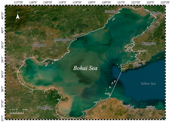
Figure 1.
A satellite remote sensing image of the study area in the Bohai Sea region.
2.2. Data Descriptions
In this study, Geo-stationary Ocean Color Imager (GOCI) Level-2A chl-a products were employed to evaluate the performance of the proposed algorithm. GOCI is the first ocean color sensor at geostationary orbit in the world, covering a total area of 2500 km × 2500 km, including the Bohai Sea. Given the high spatial resolution of 500 m and temporal resolution of 1 h (8 h per day from UTC 0:16 to 7:16), GOCI images are well suited for large-scale and high-frequency ocean monitoring. The chl-a dataset used in the experiments was collected from 1 January to 31 December 2019 within the study area, obtained from the Korea Ocean Satellite Center (KOSC) (http://kosc.kiost.ac.kr/, accessed on 17 February 2023). It should be noted that the Level-2A chl-a products have undergone standard processing procedures, including the removal of invalid data due to estimation errors or thick cloud cover [55,56]. This issue inevitably leads to data loss in the chl-a dataset, which poses challenges for continuous monitoring and analysis. Therefore, this study is motivated to develop an approach that can effectively reconstruct those missing values in the chl-a dataset and improve the utility of chl-a remote sensing products for HAB event monitoring.
A mask extraction task was first performed on each full-frame Level-2A chl-a image to generate the 2019 chl-a dataset for the Bohai Sea region. The downloaded dataset comprised 2764 images, with a resolution of 808 × 842 pixels per image and a total of 300,364 marine pixels (land pixels had already been excluded). The overall missing rate (OMR) of the dataset is 79.09%. Temporally, the spatial missing rate (SMR) of each chl-a image ranges from 6.87% to 100%. Notably, 1531 of these images have an SMR over 95%, accounting for 54.8% of the entire dataset. Spatially, the temporal missing rate (TMR) at each pixel varies from 69.36% to 100%. Among these, 20,417 pixels exhibit a TMR higher than 95%, representing 6.80% of the marine pixels. These pixels are predominantly located in nearshore shallow-water areas, as shown in Figure 2.
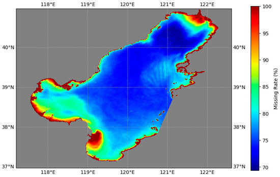
Figure 2.
Spatial distribution of the pixels TMR in 2019 chl-a original dataset of the Bohai Sea region.
Given that the EOF-based reconstruction algorithm has certain limitations on the original data, images with an SMR over 95% or pixels with a TMR over 95% are unable to provide adequate information in the spatiotemporal matrix, thus affecting the reconstruction performance [37]. Therefore, further analysis and exclusion of these highly missing images and pixels are required. The methods for checking and processing these data will be detailed in Section 2.3.2.
2.3. Methods
2.3.1. The DINEOF Algorithm
The principles of the DINEOF algorithm and implementation details used in this study can be described as follows:
- (1)
- The original dataset was stored in an matrix, where represented the number of spatial pixels and denoted the number of images. First, a base-10 logarithmic transformation was applied and the spatiotemporal mean was substracted from the matrix. Then, values at missing points were set to 0 (considered unbiased estimates), and the resulting matrix was designated as . From this, 1% of valid data were randomly selected as the cross-validation set , with the corresponding values in also set to 0.
- (2)
- The Singular Value Decomposition (SVD) was performed once on as Equation (1). Given a mode number , values at all missing points in were reconstructed following Equation (2), generating the gap-filled matrix . The Root Mean Square Error (RMSE) between the original and reconstructed values at the cross-validation set was calculated and recorded as the iteration error based on Equation (3):
The number of SVD decompositions was increased by one until the RMSE between consecutive iterations at fell below a threshold or the iteration number reached a maxinum in order to prevent dead loops and save computational time.
- (3)
- The procedure was repeated iteratively with , and the optimal number of EOFs, denoted as , was determined when the was at minimum.
- (4)
- Based on the optimal EOFs , the missing values were reconstructed and the gap-filled matrix was generated via procedure 2. Then, we added back the spatiotemporal mean and applied an exponential transformation to obtain the final reconstruction results.
2.3.2. The Implementation of the CS-DINEOF Algorithm
The strength of the DINEOF algorithm is the ability to utilize the inherent spatiotemporal consistency to extract a few modes account for the primary variations in the original data. The generated modes are used to reconstruct a comprehensive data distribution. Therefore, the input data for DINEOF should have clear and stable spatiotemporal patterns. However, in the Bohai Sea, the chl-a concentration exhibits significant variations in offshore areas influenced by human activities and terrestrial inputs, while it remains relatively stable in the open sea. This indicates the variability of spatiotemporal patterns of the chl-a concentration in the study area. The spatial distribution of the annual average concentration of the 2019 Bohai Sea chl-a data is shown in Figure 3a. Notably, the chl-a concentration in the Bohai Sea gradually decreases from the coastal areas to the open sea, with a widespread distribution of low-concentration areas, which demonstrates a stratified spatial pattern.
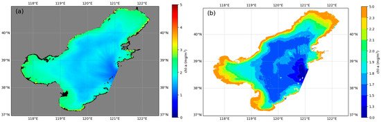
Figure 3.
Spatial distribution of average chl-a concentration in the Bohai Sea in 2019. (a) A stretch color map of chl-a concentration with a blue to red color ramp, in which blue indicates low concentration and red represents high concentration; (b) a graduated map divided into 10 levels with different intervals.
Additionally, in the DINEOF process, the spatial correlations among various points are ignored when transforming a 3-dimensional dataset into the 2-dimensional matrix. To address this limitation, we proposed a Concentration-Stratified DINEOF (CS-DINEOF) method. This approach clusters pixels with stable spatiotemporal patterns and similar distribution characteristics into the same stratum for reconstruction, thus enhancing the processing of chl-a data with complex spatiotemporal features. The overall workflow of CS-DINEOF includes four stages, as shown in Figure 4:
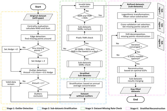
Figure 4.
Overall workflow of CS-DINEOF algorithm.
Stage 1: Outlier Detection. In the GOCI Level-2A chl-a products, due to the presence of thin mists or the boundaries of thick clouds, outliers exist in the form of speckles and edge points with significant deviations from surrounding pixel values. Therefore, in this stage, centrality evaluation based on the Median Absolute Deviation (MAD) [57] and edge detection were employed to further detect and eliminate these invalid values.
For centrality evaluation, sample sets were constructed using a spatial window of 9 × 9 pixels. The MAD of refers to the median of all absolute deviations from the sample median. The MAD and the centrality evaluation result are calculated as in Equation (4):
where is a correction factor that makes MAD a consistent estimator of the standard deviation , and is typically set at 1.4826 [58]. Following the rule, a pixel was identified as an outlier if . Using median and MAD in place of mean and standard deviation offers robustness against extreme outliers, enhancing the reliability of centrality evaluation [59].
To detect the boundaries of thick clouds, the edge detection result of each pixel with a valid value was determined by examining whether there were missing points within a 3 × 3-pixel window centered around it. If any missing points were found, was set to 3; otherwise, it was set to 0. The final result of the outlier detection was the average of and . Pixels with greater than 3 were excluded as outliers.
Stage 2: Sub-dataset Stratification. This stage embedded a coordinate–value data division strategy, which involved defining the stratification levels for the annual average chl-a concentration and subsequently dividing the Bohai Sea region into subregions, assuming that the data within each subregion would share similar spatiotemporal patterns. Specifically, the stratification levels were determined based on two key rules: (1) preserving the stratified spatial pattern of chl-a concentration and (2) ensuring balanced pixel numbers across the subregions as much as possible.
Stage 3: Dataset Missing Rate Check. As mentioned in Section 2.2, images with a high SMR and pixels with a high TMR need to be excluded for further calculations. Before CS-DINEOF reconstruction, 3 rounds of checks were required to ensure that every sub-dataset and data point could provide valid information: (1) Subregions’ SMR check: For each image, the SMR of each subregion was calculated. Only images where all subregions’ SMRs were less than 95% could be retained. Since GOCI provides 8 images per day, if more than 1 image in a day passed this check, only the image with the lowest SMR was kept. (2) TMR check: For all images passing the SMR check, the TMR of each pixel in the time series was calculated, and pixels with a TMR higher than 95% were excluded (values set to NaN). (3) Subregions’ SMR recheck: This step ensured that after the exclusion of a certain number of pixels, each image and subregion in the dataset still held valid data.
Stage 4: Stratified Reconstruction. DINEOF reconstruction was independently executed for each sub-dataset, yielding distinct optimal EOFs and corresponding RMSEs. The reconstructed sub-datasets were then systematically merged according to their positions in the original dataset, generating the final output of the CS-DINEOF process.
2.3.3. Validation Methods of Reconstruction Accuracy
To assess the accuracy of the reconstruction results based on DINEOF and CS-DINEOF algorithms, the approach described in Section 2.3.1 was employed. For each sub-dataset and time step, 1% of valid pixels were randomly selected for cross-validation. The original chl-a values at these points were recorded, and the values in the dataset under reconstruction were marked as missing. The four parameters of RMSE, Mean Absolute Error (MAE), Pearson correlation coefficient (r), and Signal-to-Noise Ratio (SNR) were used to verify the accuracy by comparing the reconstruction results with original values at cross-validation points. These parameters are defined as follows:
where represents the original chl-a values of the cross-validation set, and denotes the reconstructed chl-a values. is the number of cross-validation points.
3. Results
In this study, the 2019 chl-a dataset of the Bohai Sea region, as predefined in Section 2.2, was processed using both the ordinary DINEOF algorithm and the proposed CS-DINEOF algorithm. Both reconstruction algorithms were executed in a Python 3.9 software environment. The Lanczos operator was SVD decomposition, and the Pytorch 1.13 framework was utilized to take advantage of GPU capabilities to accelerate the speed of matrix computations.
3.1. Stratification of Sub-Datasets
According to the spatial distribution of the annual average chl-a concentration (Figure 3a) and the stratification guidelines presented in Section 2.3.2, various stratification levels were tested to obtain the optimal sub-datasets. After different attempts, 10 stratified levels were selected for the current experiments, as shown in Figure 3b. This selection achieved the most spatially reasonable stratification, effectively preserving the original spatial pattern of chl-a concentration in the study area and generating subregions with relatively balanced pixel numbers. Table 1 provides details on the sizes and missing rates of the 10 stratified sub-datasets.

Table 1.
Statistical overview of the 10 sub-datasets stratified based on annual average concentration.
It is noteworthy that subregion 3, located in the middle of the Bohai Sea, contains more pixels compared to other areas. This is due to the complex spatial distribution and high variability of chl-a in this region, influenced by terrestrial inputs from multiple sources. To preserve this intricate spatial pattern, subregion 3 was apportioned a larger number of pixels, emphasizing its significance in the complex region. Similarly, considering the higher OMR in coastal regions, subregion 10 was also allocated a relatively larger data volume, aiming to ensure an adequate supply of valid data in this region with substantial data gaps, thereby maintaining the completeness and representativeness of the sub-dataset.
3.2. Checking of Dataset Missing Rate
For 2764 original images, the SMR of each subregion was calculated first, and a total of 795 images were selected in which the SMRs of all subregions were less than 95%. Subsequently, only 139 images representing the lowest SMR for each distinct date were selected to maintain a relatively consistent time interval for further analysis. Then, a TMR check was conducted on all marine pixels, and 15,908 invalid points with a TMR over 95% were identified and marked as missing values (NaN) in all 139 images. Subsequently, the SMR for each subregion was rechecked to ensure that the SMR of each sub-dataset in the 139 images remained within acceptable limits.
The refined dataset, extracted from the original dataset passing all of the checks, included 139 images and 284,456 marine pixels, with the OMR reduced from 79.79% to 34.06% compared to the original dataset. The statistics of the dataset missing rate are presented in Figure 5. As shown in Figure 5a, the SMR per image ranges from 6.96% to 89.42%, with the majority of SMRs lower than 50%. Figure 5b indicates that the distribution of pixels TMR is similar to the original dataset (Figure 2), showing a gradual decrease from the coastal water to the open sea. However, those critically missing points have been excluded and most pixels now have TMRs below 40%, with some even lower than 20%. Figure 5c further verifies the fact that missing data in coastal areas are more severe than those in open sea areas, but the OMRs of each sub-dataset significantly decrease. In summary, compared to the original dataset, the missing data in the refined dataset were effectively restricted in both spatial and temporal dimensions.
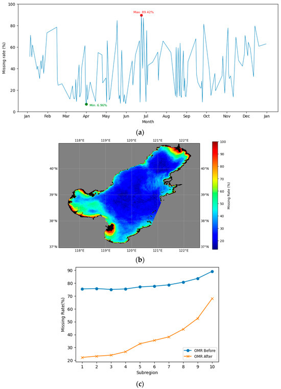
Figure 5.
Statistics of data missing from 2019 chl-a refined dataset of Bohai Sea region. (a) SMR of each chl-a image in the refined dataset. (b) Spatial distribution of TMR for each pixel point in the refined dataset. (c) Comparison of OMR for each sub-dataset before and after missing-data checks.
Notably, the number of images was reduced to 139, representing distinct dates. This reduction was considered acceptable when compared to the valid image numbers for each hour in the original dataset, which ranged from 110 to 184, as shown in Table 2.
Table 2.
Statistics of data availability for data of each hour in 2019 chl-a original dataset.
3.3. Validation and Evaluation of Reconstruction Results
Both overall reconstrution using the ordinary DINEOF algorithm and stratified reconstruction employing the CS-DINEOF algorithm were performed on the refined 2019 chl-a dataset of the Bohai Sea region. Specifically, the algorithm was configured as follows: the maximum number of EOFs was set to 20, the iterative convergence threshold was established at , and the maximum iteration steps was set to 300.
As defined in Section 2.3.3, RMSE, r, SNR and MAE were used to evaluate the reconstruction accuracy between the reconstructed values and the original values at cross-validation points. Table 3 summarizes the reconstruction performances across four validation parameters. Compared to the ordinary DINEOF algorithm, the CS-DINEOF algorithm successfully reduced the RMSE and MAE from 0.2562 mg/m3 and 0.1769 mg/m3 to 0.2281 mg/m3 and 0.1020 mg/m3, respectively. Simultaneously, r and SNR increased from 0.8910 and 15.0174 to 0.9606 and 18.0380, respectively. These results indicate that the proposed CS-DINEOF algorithm could significantly enhance the reconstruction accuracy. On the other hand, we note that there was a relatively modest improvement in RMSE, compared with the more significant improvements in the other three parameters. This issue comes from the high sensitivity of RMSE to large biases in the reconstruction of potential extreme values or outliers within the dataset.
Table 3.
The results of chl-a reconstruction on the refined dataset using the ordinary Data Interpolating Empirical Orthogonal Function (DINEOF) and the Concentration-Stratified DINEOF (CS-DINEOF) methods.
With regard to computational time (CT), the experiments demonstrate the CS-DINEOF method has a substantial advantage over the ordinary DINEOF algorithm. Because of the stratification process, the size of each sub-dataset is markedly reduced, resulting in accelerated matrix computation. With the same aforementioned computational configurations, the CT of the CS-DINEOF method is approximately 228.9% faster than that of the ordinary DINEOF method, greatly enhancing the reconstruction efficiency.
Figure 6 presents four examples of chl-a images with gaps (indicated by black spaces) on 15 February, 26 April, 22 September, and November 28 in 2019, covering four days from different seasons, with SMRs of 78.47%, 31.66%, 18.98%, and 53.46%, respectively. Figure 7, Figure 8, Figure 9 and Figure 10 show the reconstructed results using the DINEOF and CS-DINEOF methods, along with zoomed-in views of local details. As shown in Figure 7a,b, Figure 8a,b, Figure 9a,b and Figure 10a,b for data from different seasons with varying missing rates, both DINEOF and CS-DINEOF methods could fill the gaps in chl-a images with reasonable values and thus capture the comprehensive distribution of chl-a in the Bohai Sea region (except for the invalid points in coastal areas where the missing-data rate exceeds acceptable limits).
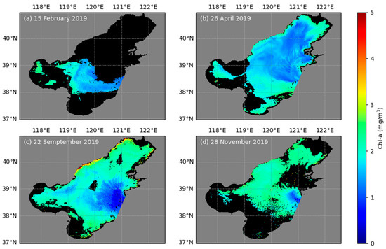
Figure 6.
Four original chl-a images on (a) 15 February, (b) 26 April, (c) 22 September, and (d) 28 November in 2019, with SMRs of 78.47%, 31.66%, 18.98%, and 53.46%, respectively.
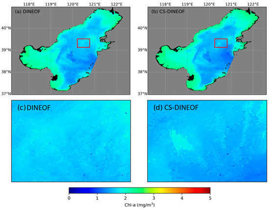
Figure 7.
The reconstruction results using (a) ordinary DINEOF and (b) CS-DINEOF on 15 February 2019. Specific local area is marked with red box in (a,b), and the corresponding zoomed-in views are presented in panels (c,d).
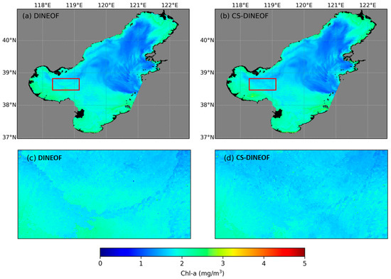
Figure 8.
The reconstruction results using (a) ordinary DINEOF and (b) CS-DINEOF on 26 April 2019. Specific local area is marked with red box in (a,b), and the corresponding zoomed-in views are shown in panels (c,d).
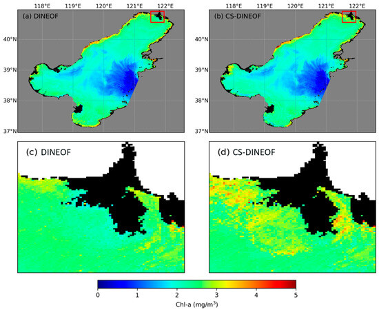
Figure 9.
The reconstruction results using (a) ordinary DINEOF and (b) CS-DINEOF on 22 September 2019. Specific local area is marked with red box in (a,b), and the corresponding zoomed-in views are shown in panels (c,d).
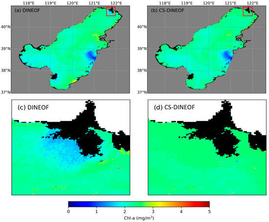
Figure 10.
The reconstruction results using (a) ordinary DINEOF and (b) CS-DINEOF on 28 November 2019. Specific local area is marked with red box in (a,b), and the corresponding zoomed-in views are shown in panels (c,d).
Figure 7c,d, Figure 8c,d, Figure 9c,d and Figure 10c,d offer zoomed-in views of specific local areas marked with red frames in Figure 7a,b, Figure 8a,b, Figure 9a,b and Figure 10a,b. Compared to the ordinary DINEOF method, the reconstructed results of the CS-DINEOF method not only reveal more local details (Figure 7c,d) but also exhibit smoother transitions (Figure 8c,d) and higher spatial coherence (Figure 9c,d and Figure 10c,d) of chl-a distribution. These comparisons demonstrate the natural advantage of the stratified reconstruction strategy employed in the CS-DINEOF algorithm. This strategy enhanced the ability to capture detailed local features while maintaining spatial coherence during the reconstruction, thus making the proposed CS-DINEOF method particularly suitable for handling chl-a data with complex spatial distributions.
As for quantitative evaluations, Figure 11 provides density scatterplots of the original and reconstructed values by the CS-DINEOF method at cross-validation points across four example data. Relevant statistical parameters, including the number of validation points (N) and the RMSE for each single image, are also annotated in the plots. Most data points are close to the 1:1 line, indicating the high consistency between the reconstructed values by CS-DINEOF and the original values at these artificially set missing points. Additionally, the low RMSEs further confirm the minimal deviations between the reconstructed values and the original data. Therefore, these results illustrate the high reliability and accuracy of the CS-DINEOF method in reconstructing chl-a data in the Bohai Sea region.
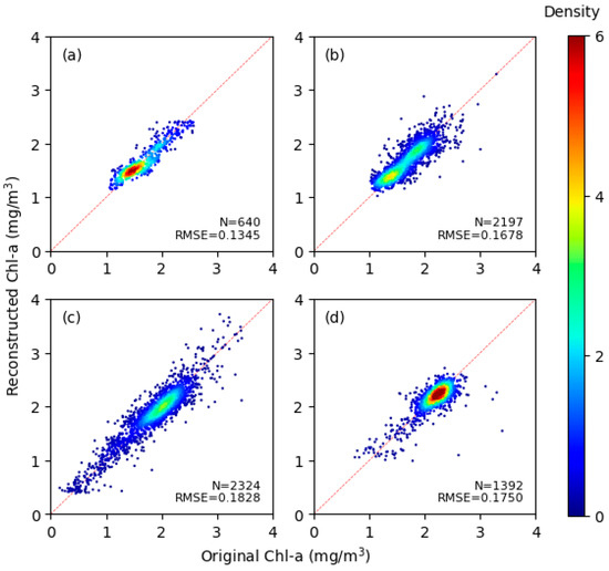
Figure 11.
Density scatterplots of original and reconstructed chl-a values by the CS-DINEOF method at cross-validation points on (a) 15 February, (b) 26 April, (c) 22 September, and (d) 28 November in 2019.
4. Discussion
4.1. Performance on Different Data SMRs
The experiments presented in Section 3.3 compared the ordinary DINEOF and the proposed CS-DINEOF methods, demonstrating that the overall reconstruction results of the CS-DINEOF method were superior to the DINEOF method. However, the impact of the data missing rate on reconstruction results should also be considered. In spatiotemporal datasets, the information required for reconstructing the missing value at a specific point is derived from data at the same location but in other images (considered as temporal modes) and from data in non-missing areas within the same images (spatial modes). As the missing rate increases, the decline in the volume of valid data diminishes the reliability of relevant information. Consequently, these spatial and temporal modes no longer dominate the variance contribution in reconstruction. Instead, missing values are approximated from the mean value or other secondary modes, thereby reducing the accuracy of the reconstruction.
To further investigate the optimization effect of the CS-DINEOF method under different missing conditions, the SMR and the RMSE between the original and reconstructed values at cross-validation points were calculated for each image in the dataset. As shown in Figure 12, although the RMSE trends of both the CS-DINEOF and ordinary DINEOF methods were similar across different SMRs, the CS-DINEOF method consistently obtained lower reconstruction errors in almost all cases, with an average reduction of 0.0281 mg/m3. Hence, it is evident that the CS-DINEOF method can achieve superior reconstruction performance over the DINEOF method under different missing conditions.
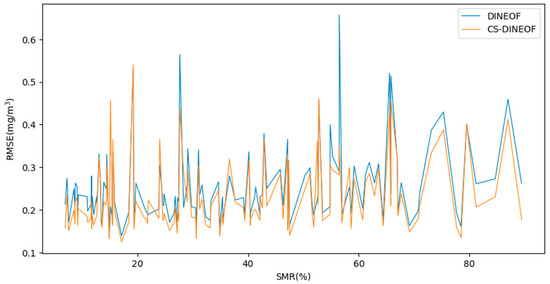
Figure 12.
RMSEs obtained from CS-DINEOF and ordinary DINEOF methods of different data SMRs of all images in the chl-a dataset.
4.2. Performance on Different Sub-Datasets
In proposing the improvement approach of CS-DINEOF, we assumed that data within subregions stratified based on annual average concentration would have similar spatiotemporal patterns. Based on this assumption, stratified reconstruction was performed, resulting in improved accuracy and efficiency compared to the ordinary DINEOF method. To assess the performance of the proposed algorithm across different sub-datasets, we carried out a stratified comparison of reconstruction results, calculating the RMSE for each sub-dataset reconstructed by both DINEOF and CS-DINEOF methods. The results, as shown in Figure 13, demonstrate that the stratified reconstruction strategy of CS-DINEOF improved the accuracy in each sub-dataset. Notably, the most substantial improvement was observed in subregion 10, suggesting that the CS-DINEOF method is more effective than DINEOF in reconstructing missing chl-a data in the coastal areas of the Bohai Sea. The reason is that the spatiotemporal patterns of chl-a in coastal areas are different from those in open-sea regions, and the CS-DINEOF method can enhance the stability of spatiotemporal patterns within stratified clusters by independently reconstructing data within each subregion, thereby significantly improving reconstruction accuracy in these regions.
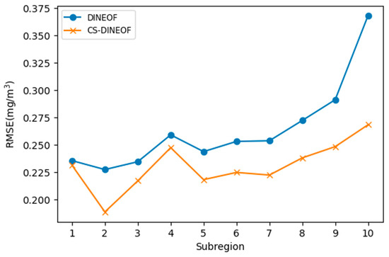
Figure 13.
RMSEs obtained from CS-DINEOF and DINEOF methods of different sub-datasets.
Further analysis was conducted to explore how the proposed CS-DINEOF algorithm achieves the enhancement of reconstruction accuracy for each sub-dataset. Table 4 presents the sub-dataset reconstruction results from the CS-DINEOF experiments. In contrast to the ordinary DINEOF, which relies on fixed optimal EOF modes to reconstruct the whole dataset, the CS-DINEOF method determines the best EOF modes for each sub-dataset. This allows every subregion to be reconstructed with the most appropriate spatiotemporal modes, thereby achieving better reconstruction accuracy. Moreover, most sub-datasets have a relatively small number of optimal modes with high variance contribution rates (VCRs). This suggests that the internal spatiotemporal correlations in these sub-datasets are robust, so that most of the original information in the dataset can be effectively captured with fewer modes. Therefore, stratification based on annual average concentration can be recognized as a straightforward and effective strategy that makes full use of the inherent spatiotemporal distribution characteristics of the chl-a data.
Table 4.
Sub-dataset reconstruction results generated from the CS-DINEOF experiments.
Finally, the total calculation time for stratified reconstruction was greatly reduced, thereby markedly improving the computational efficiency. In practical applications, given the independence of each sub-dataset, parallel reconstruction using multi-threading can further save the data processing time, therefore making the CS-DINEOF method particularly well-suited for the reconstruction of high-resolution and large-scale remote sensing datasets.
4.3. Applicability of the Improved Algorithm
Although the proposed CS-DINEOF was exclusively developed for the reconstruction of chl-a concentration in the Bohai Sea region, due to the intuitive nature of the concentration-stratified approach, it can be customized or adapted to any coastal area and open-sea applications.
However, there are limitations to the CS-DINEOF approach. In terms of data quality control, all sub-datasets are required to meet specific SMR limitations. This introduces stricter data-checking rules, resulting in a reduction in the overall data volume, particularly in the number of valid images. In fact, the refined dataset, obtained by the CS-DINEOF quality control procedure, represents the highest-quality data in the original dataset. Stratified reconstruction applied to this refined dataset achieves high-precision and high-efficiency reconstruction, but with relatively diminished temporal continuity. If enhanced temporal continuity is required for better monitoring the continuous changes in practical applications, it is feasible to implement the ordinary DINEOF on other data in the dataset that do not meet the SMR limitation for sub-datasets but have an acceptable OMR. By incorporating the DINEOF reconstruction results into the high-quality CS-DINEOF results, it can further enhance the overall spatiotemporal continuity and practical application value of the final gap-free datasets.
5. Conclusions
In this study, an improved DINEOF algorithm, termed Concentration-Stratified DINEOF, was developed to specifically address the challenges of high resolution, large data volume, and uneven spatiotemporal distribution of chl-a concentration in the Bohai Sea region. This method employed a coordinate–value correlative data division strategy, which stratified the Bohai Sea region into 10 subregions based on the annual average concentration of chl-a, in order to cluster points with stable spatiotemporal patterns and similar distribution characteristics into separate sub-datasets. Outlier detection and missing rate checks were performed in each sub-dataset for data quality control. In the reconstruction process, rather than relying on a fixed optimal EOF mode for the whole dataset, each sub-dataset was individually reconstructed using its respective optimal EOF mode, generating separate reconstruction results which were then merged to form a complete and final reconstructed image. The proposed CS-DINEOF method was successfully applied to reconstruct the 2019 GOCI Level-2A chl-a products of the Bohai Sea region. Compared to the ordinary DINEOF method, CS-DINEOF achieved a higher reconstruction accuracy, with notable improvements in all four validation parameters (RMSE, MAE, r, and SNR). Additionally, by reducing the volume of data in each sub-dataset via stratification, CS-DINEOF significantly enhanced the reconstruction efficiency, improving computational efficiency by approximately 228.9% under the same configuration. Although incorporating strict data quality control steps into CS-DINEOF would lead to a substantial reduction in data volume, particularly in the number of valid images, and the algorithm’s sensitivity to extreme values somewhat limited RMSE improvement, further comparative analysis and discussions demonstrated that CS-DINEOF outperformed the ordinary DINEOF method across different missing conditions and sub-datasets. This illustrates that although the stratification based on annual average concentration only represents a simple data distribution pattern, it can effectively utilize the inherent spatiotemporal correlations within the original data to enhance reconstruction performance. The experiments conducted in this paper suggest that CS-DINEOF-based remote sensing image reconstruction can not only provide smoother transitions and higher spatial correlation but also reveal more local details, which are significantly valuable for supporting research on water quality and HABs in the Bohai Sea region.
Author Contributions
Conceptualization, R.Q. and T.H.; methodology, R.Q. and T.H.; software, T.H. and Z.X.; validation, R.Q. and T.H.; data curation, T.H.; writing—original draft preparation, T.H.; writing—review and editing, R.Q. and T.H.; visualization, T.H.; supervision, R.Q.; project administration, R.Q.; funding acquisition, R.Q. All authors have read and agreed to the published version of the manuscript.
Funding
This work was funded by the National Key Research and Development Program of China (No. 2019YFC1407902), the Innovation Program of Shanghai Municipal Education Commission (2021-01-07-00-07-E00093), and the Interdisciplinary Project in Ocean Research of Tongji University (2022-2-ZD-04).
Institutional Review Board Statement
Not applicable.
Informed Consent Statement
Not applicable.
Data Availability Statement
The GOCI Level-2A chl-a products utilized in this work can be obtained from the Korea Ocean Satellite Center (KOSC) (http://kosc.kiost.ac.kr/).
Acknowledgments
The authors would like to thank the Korea Ocean Satellite Center (KOSC) for providing the GOCI data.
Conflicts of Interest
The authors declare no conflicts of interest.
References
- Mcowen, C.J.; Cheung, W.W.; Rykaczewski, R.R.; Watson, R.A.; Wood, L.J. Is fisheries production within L arge M arine E cosystems determined by bottom-up or top-down forcing? Fish Fish. 2015, 16, 623–632. [Google Scholar] [CrossRef]
- Rostam, N.A.P.; Malim, N.H.A.H.; Abdullah, R.; Ahmad, A.L.; Ooi, B.S.; Chan, D.J.C. A complete proposed framework for coastal water quality monitoring system with algae predictive model. IEEE Access 2021, 9, 108249–108265. [Google Scholar] [CrossRef]
- IOC-UNESCO. What Are Harmful Algae. Available online: https://hab.ioc-unesco.org/what-are-harmful-algae (accessed on 17 December 2023).
- Na, L.; Shaoyang, C.; Zhenyan, C.; Xing, W.; Yun, X.; Li, X.; Yanwei, G.; Tingting, W.; Xuefeng, Z.; Siqi, L. Long-term prediction of sea surface chlorophyll-a concentration based on the combination of spatio-temporal features. Water Res. 2022, 211, 118040. [Google Scholar] [CrossRef]
- Qin, R.; Yang, S.; Xu, Z.; Hong, T. Development of a web-based modelling framework for harmful algal blooms transport simulation using open-source technologies. J. Environ. Manag. 2023, 325, 116616. [Google Scholar] [CrossRef]
- Kallio, K.; Koponen, S.; Pulliainen, J. Feasibility of airborne imaging spectrometry for lake monitoring—A case study of spatial chlorophyll a distribution in two meso-eutrophic lakes. Int. J. Remote Sens. 2003, 24, 3771–3790. [Google Scholar] [CrossRef]
- Huot, Y.; Babin, M.; Bruyant, F.; Grob, C.; Twardowski, M.; Claustre, H. Does chlorophyll a provide the best index of phytoplankton biomass for primary productivity studies? Biogeosci. Discuss. 2007, 4, 707–745. [Google Scholar]
- Zou, W.; Zhu, G.; Cai, Y.; Vilmi, A.; Xu, H.; Zhu, M.; Gong, Z.; Zhang, Y.; Qin, B. Relationships between nutrient, chlorophyll a and Secchi depth in lakes of the Chinese Eastern Plains ecoregion: Implications for eutrophication management. J. Environ. Manag. 2020, 260, 109923. [Google Scholar] [CrossRef]
- Yang, X.; Huang, M.; Bai, K. Simulation System of Lake Eutrophication Evolution based on RS & GIS Technology—A Case Study in Wuhan East Lake. In IOP Conference Series: Earth and Environmental Science; IOP Publishing: Bristol, UK, 2020; p. 012002. [Google Scholar]
- O’Reilly, J.E.; Maritorena, S.; Mitchell, B.G.; Siegel, D.A.; Carder, K.L.; Garver, S.A.; Kahru, M.; McClain, C. Ocean color chlorophyll algorithms for SeaWiFS. J. Geophys. Res. Ocean. 1998, 103, 24937–24953. [Google Scholar] [CrossRef]
- Abbas, M.M.; Melesse, A.M.; Scinto, L.J.; Rehage, J.S. Satellite estimation of chlorophyll-a using moderate resolution imaging spectroradiometer (MODIS) sensor in shallow coastal water bodies: Validation and improvement. Water 2019, 11, 1621. [Google Scholar] [CrossRef]
- Oelen, A.; van Aart, C.J.; De Boer, V. Measuring Surface Water Quality Using a Low-Cost Sensor Kit within the Context of Rural Africa. In P-ICT4D@ WebSci; Vrije Universiteit Amsterdam: Amsterdam, The Netherlands, 2018. [Google Scholar]
- Binh, N.A.; Hoa, P.V.; Thao, G.T.P.; Duan, H.D.; Thu, P.M. Evaluation of Chlorophyll-a estimation using Sentinel 3 based on various algorithms in southern coastal Vietnam. Int. J. Appl. Earth Obs. Geoinf. 2022, 112, 102951. [Google Scholar] [CrossRef]
- Bernard, S.; Kudela, R.M.; Robertson Lain, L.; Pitcher, G. Observation of Harmful Algal Blooms with Ocean Colour Radiometry; International Ocean Colour Coordinating Group (IOCCG): Dartmouth, NS, Canada, 2021. [Google Scholar]
- Smith, M.E.; Lain, L.R.; Bernard, S. An optimized chlorophyll a switching algorithm for MERIS and OLCI in phytoplankton-dominated waters. Remote Sens. Environ. 2018, 215, 217–227. [Google Scholar] [CrossRef]
- Gordon, H.R.; Clark, D.K.; Brown, J.W.; Brown, O.B.; Evans, R.H.; Broenkow, W.W. Phytoplankton pigment concentrations in the Middle Atlantic Bight: Comparison of ship determinations and CZCS estimates. Appl. Opt. 1983, 22, 20–36. [Google Scholar] [CrossRef]
- Ahn, Y.-H.; Shanmugam, P. Detecting the red tide algal blooms from satellite ocean color observations in optically complex Northeast-Asia Coastal waters. Remote Sens. Environ. 2006, 103, 419–437. [Google Scholar] [CrossRef]
- Gower, J.F.; Brown, L.; Borstad, G. Observation of chlorophyll fluorescence in west coast waters of Canada using the MODIS satellite sensor. Can. J. Remote Sens. 2004, 30, 17–25. [Google Scholar] [CrossRef]
- Moses, W.J.; Gitelson, A.A.; Berdnikov, S.; Povazhnyy, V. Estimation of chlorophyll-a concentration in case II waters using MODIS and MERIS data—Successes and challenges. Environ. Res. Lett. 2009, 4, 045005. [Google Scholar] [CrossRef]
- Yu, X.; Shen, J.; Zheng, G.; Du, J. Chlorophyll-a in Chesapeake Bay based on VIIRS satellite data: Spatiotemporal variability and prediction with machine learning. Ocean. Model. 2022, 180, 102119. [Google Scholar] [CrossRef]
- Zhang, Y.; Hu, M.; Shi, K.; Zhang, M.; Han, T.; Lai, L.; Zhan, P. Sensitivity of phytoplankton to climatic factors in a large shallow lake revealed by column-integrated algal biomass from long-term satellite observations. Water Res. 2021, 207, 117786. [Google Scholar] [CrossRef]
- Yussof, F.N.; Maan, N.; Md Reba, M.N. LSTM networks to improve the prediction of harmful algal blooms in the West Coast of sabah. Int. J. Environ. Res. Public Health 2021, 18, 7650. [Google Scholar] [CrossRef]
- Zhao, W.; Zhou, B.; Liu, H.; Li, H.; Jiang, D.; Ji, M. BP neural network-based short-term prediction of chlorophyll concentration inmainstreamof Haihe River. Water Resour. Hydropower Eng. 2017, 48, 134–140. [Google Scholar]
- Konik, M.; Kowalewski, M.; Bradtke, K.; Darecki, M. The operational method of filling information gaps in satellite imagery using numerical models. Int. J. Appl. Earth Obs. Geoinf. 2019, 75, 68–82. [Google Scholar] [CrossRef]
- Ackerman, S.A.; Strabala, K.I.; Menzel, W.P.; Frey, R.A.; Moeller, C.C.; Gumley, L.E. Discriminating clear sky from clouds with MODIS. J. Geophys. Res. Atmos. 1998, 103, 32141–32157. [Google Scholar] [CrossRef]
- Kondrashov, D.; Ghil, M. Spatio-temporal filling of missing points in geophysical data sets. Nonlinear Process. Geophys. 2006, 13, 151–159. [Google Scholar] [CrossRef]
- Wang, M.; Shi, W. Cloud masking for ocean color data processing in the coastal regions. IEEE Trans. Geosci. Remote Sens. 2006, 44, 3196–3205. [Google Scholar] [CrossRef]
- Wang, M.; Bailey, S.W. Correction of sun glint contamination on the SeaWiFS ocean and atmosphere products. Appl. Opt. 2001, 40, 4790–4798. [Google Scholar] [CrossRef] [PubMed]
- Liu, X.; Wang, M. Gap filling of missing data for VIIRS global ocean color products using the DINEOF method. IEEE Trans. Geosci. Remote Sens. 2018, 56, 4464–4476. [Google Scholar] [CrossRef]
- He, R.; Weisberg, R.H.; Zhang, H.; Muller-Karger, F.E.; Helber, R.W. A cloud-free, satellite-derived, sea surface temperature analysis for the West Florida Shelf. Geophys. Res. Lett. 2003, 30, 1811. [Google Scholar] [CrossRef]
- Schoellhamer, D.H. Singular spectrum analysis for time series with missing data. Geophys. Res. Lett. 2001, 28, 3187–3190. [Google Scholar] [CrossRef]
- Schneider, T. Analysis of incomplete climate data: Estimation of mean values and covariance matrices and imputation of missing values. J. Clim. 2001, 14, 853–871. [Google Scholar] [CrossRef]
- Lu, G.Y.; Wong, D.W. An adaptive inverse-distance weighting spatial interpolation technique. Comput. Geosci. 2008, 34, 1044–1055. [Google Scholar] [CrossRef]
- Bhattacharjee, S.; Mitra, P.; Ghosh, S.K. Spatial interpolation to predict missing attributes in GIS using semantic kriging. IEEE Trans. Geosci. Remote Sens. 2013, 52, 4771–4780. [Google Scholar] [CrossRef]
- Rossi, R.E.; Dungan, J.L.; Beck, L.R. Kriging in the shadows: Geostatistical interpolation for remote sensing. Remote Sens. Environ. 1994, 49, 32–40. [Google Scholar] [CrossRef]
- Beckers, J.-M.; Rixen, M. EOF calculations and data filling from incomplete oceanographic datasets. J. Atmos. Ocean. Technol. 2003, 20, 1839–1856. [Google Scholar] [CrossRef]
- Alvera-Azcárate, A.; Barth, A.; Rixen, M.; Beckers, J.-M. Reconstruction of incomplete oceanographic data sets using empirical orthogonal functions: Application to the Adriatic Sea surface temperature. Ocean. Model. 2005, 9, 325–346. [Google Scholar] [CrossRef]
- Henn, B.; Raleigh, M.S.; Fisher, A.; Lundquist, J.D. A comparison of methods for filling gaps in hourly near-surface air temperature data. J. Hydrometeorol. 2013, 14, 929–945. [Google Scholar] [CrossRef]
- Huynh, H.-N.T.; Alvera-Azcárate, A.; Barth, A.; Beckers, J.-M. Reconstruction and analysis of long-term satellite-derived sea surface temperature for the South China Sea. J. Oceanogr. 2016, 72, 707–726. [Google Scholar] [CrossRef]
- Sarah, C.M.; Laura, J.N.; James, S.; Matthew, J.O.; Josh, K.; Michael, C. Persistent upwelling in the Mid-Atlantic Bight detected using gap-filled high-resolution satellite SST. Remote Sens. Environ. 2021, 26, 112487. [Google Scholar]
- Hu, R.; Zhao, J. Sea surface salinity variability in the western subpolar North Atlantic based on satellite observations. Remote Sens. Environ. 2022, 281, 113257. [Google Scholar] [CrossRef]
- Miles, T.N.; He, R. Temporal and spatial variability of Chl-a and SST on the South Atlantic Bight: Revisiting with cloud-free reconstructions of MODIS satellite imagery. Cont. Shelf Res. 2010, 30, 1951–1962. [Google Scholar] [CrossRef]
- Li, D.; Gao, Z.; Wang, Y. Research on the long-term relationship between green tide and chlorophyll-a concentration in the Yellow Sea based on Google Earth Engine. Mar. Pollut. Bull. 2022, 177, 113574. [Google Scholar] [CrossRef]
- Hilborn, A.; Costa, M. Applications of DINEOF to satellite-derived chlorophyll-a from a productive coastal region. Remote Sens. 2018, 10, 1449. [Google Scholar] [CrossRef]
- Wang, Y.; Liu, D. Reconstruction of satellite chlorophyll-a data using a modified DINEOF method: A case study in the Bohai and Yellow seas, China. Int. J. Remote Sens. 2014, 35, 204–217. [Google Scholar] [CrossRef]
- Ping, B.; Su, F.; Meng, Y. Reconstruction of satellite-derived sea surface temperature data based on an improved DINEOF algorithm. IEEE J. Sel. Top. Appl. Earth Obs. Remote Sens. 2015, 8, 4181–4188. [Google Scholar] [CrossRef]
- Ping, B.; Su, F.; Meng, Y. An improved DINEOF algorithm for filling missing values in spatio-temporal sea surface temperature data. PLoS ONE 2016, 11, e0155928. [Google Scholar] [CrossRef] [PubMed]
- Liu, X.; Wang, M. Filling the gaps of missing data in the merged VIIRS SNPP/NOAA-20 ocean color product using the DINEOF method. Remote Sens. 2019, 11, 178. [Google Scholar] [CrossRef]
- Liu, X.; Wang, M. Global daily gap-free ocean color products from multi-satellite measurements. Int. J. Appl. Earth Obs. Geoinf. 2022, 108, 102714. [Google Scholar] [CrossRef]
- Yao, Z.; He, R.; Bao, X.; Wu, D.; Song, J. M2 tidal dynamics in Bohai and Yellow Seas: A hybrid data assimilative modeling study. Ocean. Dyn. 2012, 62, 753–769. [Google Scholar] [CrossRef]
- Chen, B.; Smith, S.L. Optimality-based approach for computationally efficient modeling of phytoplankton growth, chlorophyll-to-carbon, and nitrogen-to-carbon ratios. Ecol. Model. 2018, 385, 197–212. [Google Scholar] [CrossRef]
- Wang, J.; Kuang, C.; Ou, L.; Zhang, Q.; Qin, R.; Fan, J.; Zou, Q. A Simple Model for a Fast Forewarning System of Brown Tide in the Coastal Waters of Qinhuangdao in the Bohai Sea, China. Appl. Sci. 2022, 12, 6477. [Google Scholar] [CrossRef]
- Ma, S.; Zhang, X.; Ding, C.; Han, W.; Lu, Y. Comparison of the spatiotemporal variation of Chl-a in the East China Sea and Bohai Sea based on long time series satellite data. In Proceedings of the 2021 9th International Conference on Agro-Geoinformatics (Agro-Geoinformatics), Shenzhen, China, 26–29 July 2021; pp. 1–6. [Google Scholar]
- Zhao, N.; Zhang, G.; Zhang, S.; Bai, Y.; Ali, S.; Zhang, J. Temporal-spatial distribution of chlorophyll-a and impacts of environmental factors in the Bohai Sea and Yellow Sea. IEEE Access 2019, 7, 160947–160960. [Google Scholar] [CrossRef]
- Park, Y.; Ahn, Y.; Han, H.; Yang, H.; Moon, J.; Ahn, J.; Lee, B.; Min, J.; Lee, S.; Kim, K. GOCI Level 2 Ocean Color Products (GDPS 1.3) Brief Algorithm Description; Korea Ocean Satellite Center (KOSC): Ansan, Republic of Korea, 2014; pp. 24–40. [Google Scholar]
- Jeon, H.-K.; Cho, H.Y. Missing Pattern Analysis of the GOCI-I Optical Satellite Image Data. Ocean. Polar Res. 2022, 44, 179–190. [Google Scholar]
- Hampel, F.R. The influence curve and its role in robust estimation. J. Am. Stat. Assoc. 1974, 69, 383–393. [Google Scholar] [CrossRef]
- Iglewicz, B.; Hoaglin, D.C. Volume 16: How to Detect and Handle Outliers; Quality Press: Welshpool, Australia, 1993. [Google Scholar]
- Qi, M.; Fu, Z.; Chen, F. Outliers detection method of multiple measuring points of parameters in power plant units. Appl. Therm. Eng. 2015, 85, 297–303. [Google Scholar] [CrossRef]
Disclaimer/Publisher’s Note: The statements, opinions and data contained in all publications are solely those of the individual author(s) and contributor(s) and not of MDPI and/or the editor(s). MDPI and/or the editor(s) disclaim responsibility for any injury to people or property resulting from any ideas, methods, instructions or products referred to in the content. |
© 2024 by the authors. Licensee MDPI, Basel, Switzerland. This article is an open access article distributed under the terms and conditions of the Creative Commons Attribution (CC BY) license (https://creativecommons.org/licenses/by/4.0/).