Cascade-Forward, Multi-Parameter Artificial Neural Networks for Predicting the Energy Efficiency of Photovoltaic Modules in Temperate Climate

Featured Application

Artificial Neural Networks have confirmed applications in predicting PV system energetic efficiency.

Abstract

Solar energy is a promising and efficient source of electricity in countries with stable and high sunshine duration. However, in less favorable conditions, for example in continental, temperate climates, the process requires optimization to be cost-effective. This cannot be done without the support of appropriate mathematical and numerical methods. This work presents a procedure for the construction and optimization of an artificial neural network (ANN), along with an example of its practical application under the conditions mentioned above. In the study, data gathered from a photovoltaic system in 457 consecutive days were utilized. The data includes measurements of generated power, as well as meteorological records. The cascade-forward ANN was trained with a resilient backpropagation procedure and sum squared error as a performance function. The final ANN has two hidden layers with nine and six nodes. This resulted in a relative error of 10.78% and R² of 0.92–0.97 depending on the data sample. The case study was used to present an example of the potential application of the tool. This approach proved the real benefits of the optimization of energy consumption.

1. Introduction

The growing problem with conventional fuels and concern for environmental protection combined with increasing demand for energy have contributed to the development of renewable energy technologies. Solar energy conversion devices are still being improved and the availability of photovoltaic technology is increasing [1]. The spread of photovoltaic energy is in line with the climate goals of the European Union. Poland is also seeing an increase in solar energy. The data from the Energy Regulatory Office shows that photovoltaic power attached to the network at the end of 2014 was 20 MW, and at the end of 2020 was almost 4 GW. This means that within 6 years, it increased almost 200-fold. This is due to the increasing interest of the prosumers in this source of energy in households. The energy policy pursued by the Polish Government aims at strengthening the security and energy independence of the country, focusing on numerous programs co-financing the purchase of PV installations [2]. According to Solar Power Europe, in 2021, Poland was in fourth place in terms of the capacity of installed PV in the European Union after Germany (4.74 GW), the Netherlands (3 GW) and Spain (2.8 GW) [3].

In order to meet the assumptions of the RED II Directive [4], at least double the installed capacity of solar energy is needed. This is due to the fact that within the community as a whole, energy production from solar radiation (10 percent) is still less than from coal, which accounted for 14 percent of the EU mix in June–July 2021 (58 TWh). Currently, the solar market is poised to support the required growth. The global average levelized cost of electricity (LCOE) for solar PV has fallen from $381/MWh in 2010 to $57/MWh in 2020 [5]. The slow development can be attributed mainly to two issues: those related to energy security and coal-based power generation, and the interests of large mining corporations [6].

The parameter that is used to determine the potential of a given location for setting up a PV installation is insolation. It determines the amount of solar radiation per unit area per year and is dependent on two components. One of them is predictable and is related to the rotation of the Earth around the Sun and the latitude of the examined location. So, it is a constant cycle, repeated every year. Based on it, the maximum value of insolation can be determined. The second component is stochastic and depends on the occurring atmospheric conditions. Another quantity influenced by these two components is insolation. It is defined as the time during which the sun’s rays fall directly on a given location during the year [7]. A high insolation value has a beneficial effect on the power generation of PV modules and determines the annual amount of time the panel can operate at the power specified by the manufacturer. The exclusive quantity that includes only a weather-dependent component is relative insolation. It is a value of insolation related to the maximum insolation that can occur at a given latitude. For each year, the value of maximum insolation is constant and, like insolation, is expressed in hours per year. Therefore, relative insolation is expressed in percentage, and in Poland, it ranges from 35 to 48% [8].

The real influence on the generated energy during the year has the average intensity of solar radiation falling on 1 m² multiplied by the number of working hours of the module under study [7]. This parameter takes into account both the direct and indirect impact of the sun on the panel surfaces. Poland is located in the temperate climate zone, warm group, transitional type. The highest insolation in Poland is found in the Lubelskie, Podkarpackie, Małopolskie, Opolskie, Dolnośląskie, Łódzkie provinces, as well as the southern parts of the Mazowieckie and Wielkopolskie provinces, with the highest values in the southern part of the Lubelskie province amounting to nearly 1100 $\frac{\mathrm{k}\mathrm{W}\mathrm{h}}{{\mathrm{m}}^2·\mathrm{y}\mathrm{e}\mathrm{a}\mathrm{r}}$. In central Poland, the insolation ranges from 1022 to 1048 $\frac{\mathrm{k}\mathrm{W}\mathrm{h}}{{\mathrm{m}}^2·\mathrm{y}\mathrm{e}\mathrm{a}\mathrm{r}}$. In the rest of the country, the insolation is slightly below 1000 $\frac{\mathrm{k}\mathrm{W}\mathrm{h}}{{\mathrm{m}}^2·\mathrm{y}\mathrm{e}\mathrm{a}\mathrm{r}}$. The least insolation in Poland occurs in the Zachodniopomorskie and Pomorskie provinces. The city with the highest annual electricity received from photovoltaics, where the installation with a capacity of 1 kW produces an annual average of 1096 $\frac{\mathrm{k}\mathrm{W}\mathrm{h}}{{\mathrm{m}}^2·\mathrm{y}\mathrm{e}\mathrm{a}\mathrm{r}}$, is Rzeszów followed by Lublin and Tarnów (1084 $\frac{\mathrm{k}\mathrm{W}\mathrm{h}}{{\mathrm{m}}^2·\mathrm{y}\mathrm{e}\mathrm{a}\mathrm{r}}$ each) [9,10].

For example, in Malaysia, a country with high sunshine levels, solar energy is the main alternative system for electricity generation that reduces greenhouse gases [11,12]. Malaysia lies in the equatorial climate belt and consists of two regions: Peninsular West and East Malaysia, with very high solar potential (22–24 $\frac{\mathrm{M}\mathrm{J}}{{\mathrm{m}}^2}$ and 14–24 $\frac{\mathrm{M}\mathrm{J}}{{\mathrm{m}}^2}$ per day [13]) for electricity generation. In order to compare the conditions in Poland and Malaysia, the values of daily insolation were converted into annual insolation. The value for Malaysia varies between 1423 $\frac{\mathrm{k}\mathrm{W}\mathrm{h}}{{\mathrm{m}}^2·\mathrm{y}\mathrm{e}\mathrm{a}\mathrm{r}}$ and 2435 $\frac{\mathrm{k}\mathrm{W}\mathrm{h}}{{\mathrm{m}}^2·\mathrm{y}\mathrm{e}\mathrm{a}\mathrm{r}}$. In addition, the energy produced each day varies only slightly throughout the year. This is due to the length of the day in the equatorial belt. Its length throughout the year is practically unchanged; the longest day lasts for 12:18 h and the shortest for 11:56 h. In this case, it is much easier to design installations to meet the energy needs of the consumer, and no long-term energy storage is required. Very good conditions for electricity generation from the sun could meet the energy needs of the population at a projected level of 23.1 GW in 2019, which was a 39.47% increase over the peak demand in 2013 [14].

The degree of efficiency of the module under specific operating conditions has a key influence on the output power. In most cases, e.g., due to the conditions in Europe, Standard Test Conditions (STC) are taken into account. They define the module working temperature at 25 °C and the amount of solar energy falling on the panel at 1000 $\frac{\mathrm{W}}{{\mathrm{m}}^2}$ [15]. Therefore, it can be assumed that the efficiency given by the manufacturer is the “output efficiency”. Its value will change depending on changes in parameters specified by STC. Its value is directly influenced by manufacturing technology and materials used for production. Poland is a favorable area for investment in photovoltaic systems because a cooler than tropical climate is conducive to converting solar energy into electricity. Annual insolation in Poland amounts to an average of 990 $\frac{\mathrm{k}\mathrm{W}\mathrm{h}}{{\mathrm{m}}^2}$. The sunniest months are June, July, and August—these months account for about 43% of annual radiation. It has been estimated that about 77% of the annual radiation energy in Poland falls on the six warmer months of the year (April to September) and only 23% from October to March. It can be assumed that the atmospheric conditions in Poland are optimal, because, contrary to popular belief, hot regions of the world and prolonged heat are not conducive to energy production from photovoltaics. The temperature of the module during its operation is inversely proportional to its efficiency. Its influence on the operation of the installation is significant; therefore, a value of 25 °C, calculated as the most suitable, is given for the rated conditions (Normal Operating Cell Temperature and Standard Test Conditions). Each photovoltaic module manufacturer should declare the value of such parameters as temperature and power factor. It is defined as the value by which the efficiency will change when the cell temperature changes by 1 °C [16].

From the formula presented by Duffie, Erbs, and Graham, it can be seen that the module temperature depends on many factors related to the prevailing conditions (irradiance and ambient temperature) and the properties of the materials the photovoltaic module is made of (module efficiency, power temperature coefficient, absorbance, and transmittance) [17,18,19]. In order to determine the module temperature even more precisely, it is necessary to take into account the heat released when current flows through the semiconductor region and, if wind is present, the heat transfer in forced convection [20]. Although the resistance value in semiconductors decreases with increasing temperature, the efficiency of the cell decreases. In most electrical devices, resistance is responsible for most of the losses in the flow of electricity. This is not the case with photovoltaic cells. The main source of energy loss is the decrease in the mobility of electrons and holes as the temperature of semiconductors increases under the influence of voltage forcing. In the case of monocrystalline cells, the production process involves, among other things, the purification of the material to a silicon content of 99%. Particularly visible mobility changes occur with a low dopant content in crystalline silicon. However, they are added to the semiconductor p layer to separate the positive (p) and negative (n) junction layers. A junction containing dopants (e.g., Al or B) has one of the covalent bonds decomposed. This causes the formation of holes and, under the influence of incident photons on the n junction, the appearance of a potential difference and current flow [8]. This is the main reason for the decrease in cell efficiency for operation above 25 °C. If the module temperature drops below the rated conditions, the instantaneous efficiency may exceed the rated efficiency (provided that the other parameters included in the STC remain constant). This can occur in winter when the temperature drops below 0 °C or during adequate cloud cover because part of solar radiation is reflected and falls into the photovoltaic panel. Usually, the state of higher efficiency lasts no longer than 1 h.

Most of the studies conducted from 1991 to 2016 focused only on some factors related to PV panels. In addition, these studies did not reveal the direct quantitative impact of each factor on panel performance but rather focused more on showing the overall increase or decrease in the impact of certain factors, both environment-related and internal factors [21,22].

Mathematical models can be used for local sunshine forecasting [23]. Research carried out in Portugal has made it possible to generate improved insolation maps. The release of the results had an impact on the future planning of photovoltaic farms, among other things [24]. It is also possible to use neural networks for global insolation forecasting. One model considered meteorological data from several variables: mean daily air temperature, insolation, evaporation, and wind speed [25]. Similar results were obtained from the model by Al-Alawi and Al-Hinai [26]. However, they are valuable as they take into account climatological variables generating negligible errors of 5–7.5% for different areas.

The next stage of scientific development in the application of mathematical models has been the consideration of variable parameters of PV installations. The main application concerns the design of hybrid energy systems and off-grid installations, taking into account different parameters. An interesting concept of an off-grid installation designed taking into account results from a neural network model is presented in Hassan’s paper [27]. In the study, baseline mathematical variables were defined, namely the electrical load profile, solar radiation, air temperature, and wind speed. Different photovoltaic operating states (on-grid and off-grid), different states related to the angle of tilt of the modules (constant—average annual optimum, variable), and the level of degradation of PV modules over the years were simulated. Another study by L. Fara et al. [28] applied modeling based on modular blocks to design a stand-alone PV system in an isolated area in Romania. In addition to the PV system, energy storage was used to provide energy at times of low power generation.

Another well-known application of ANNs and other mathematical models is the prediction of energy generation and PV panel operation [29,30]. Some studies focused on optimizing energy generation by varying the operating maximum power point (MPP) of PV modules [31]. Later studies present higher optimization accuracy or consider more variables, e.g., by presenting different selection methods for meteorological variables [32,33,34]. A study by Narasimman et al. [35] presents results for an ANN-performed optimization in a 5 MW solar farm system. On such a large scale, the effects of the model are definitely more visible.

A very extensive and at the same time insightful analysis of the use of mathematical models for the design, operation, fault identification, and forecasting of renewable energy generation has been conducted within the framework of monographs [33,36]. These works summarily present a review of about 150 articles, and this allowed the authors to present new findings in the analyzed field. Additionally, a very broad literature review is presented in the monograph, although it deals with technology that was commercially available before 2017 [37]. Among other things, it presents recommendations for the application of specific computational methods for selected research problems.

The research presented in this article is the result of exceedingly high interest in solar energy conversion technology. The literature review prepared confirms the need for and very wide range of advanced mathematical models [38]. This technology is a solution to many problems faced by the energy industry and the increasing population of mankind. In the face of climate change, the need to preserve the environment and improve the quality of life of people is undertaken not only in the professional power industry but also in the transport industry and prosumer energy systems. Photovoltaics as an energy source with a satisfactory return on investment even for very low installed capacity is the most widely developed technology. However, the whole production process must be optimized for both economic and local legal reasons. This paper describes an attempt to systematize the influence of weather conditions on energy production in a temperate climate using artificial neural network (ANN) modeling [39]. The use of basic meteorological data such as predicted insolation, temperature, and humidity is now well established in the literature [35]. Compared to such studies, an element of novelty in this work is the use of additional information such as the day number of the year, corresponding to the intermediate angle of the sun. The use of such custom data allows for improved modeling accuracy, especially for the winter period which is important in temperate climates. The presented methodology is designed to adjust energy consumption based on predicted production. This novel approach can have numerous benefits, such as maximizing power plant revenue as well as reducing the carbon footprint of an industrial, agricultural, or household facility (in the case of domestic PV installations). This work will also provide an example of how to use the aforementioned tool to optimize energy use for a model household and minimize the amount of energy purchased from the grid.

2. Materials and Methods

2.1. Measurements, Data Collection, and Model Type Selection

Photovoltaics is developing extremely fast and nowadays we can talk about many different types of models and approaches, depending on the final application of energy yield forecasts. The forecasts can refer to a single PV plant, a group of plants over a larger geographical area, or different time horizons [40]. 0–6 h ahead forecasts and day-ahead forecasts are crucial for successful grid integration [41]. Physical weather forecasting methods use weather forecasts, PV models, and characteristics, while statistical methods rely mainly on past data and numerical methods, with little or no dependence on PV models [42]. The increase in the number of PV power plants connected to the power system has led to increased interest in the development of various PV power forecasting models. The models can be based on advanced techniques such as artificial neural networks (ANNs) [43,44], as well as support vector machines [45,46] or various hybrid models [47,48]. In this study, the ANN model was used.

In choosing a working plant suitable for the study, two main factors were considered. The first one is related to weather conditions, and these are directly related to the location of the installation. In the case considered in this study, the PV system was installed in western Poland, in the Wielkopolskie voivodeship, in Poznan County, Komorniki municipality. According to the research conducted by the Institute of Meteorology and Water Management in Poland, the sunlight conditions in this area are similar to the average sunlight conditions in Poland [8]. Thus, it can be concluded that the results of the analysis will be similar to the average results obtained in Poland, which is important for the objectivity of the study conducted. The second crucial factor in selecting a suitable photovoltaic installation for the study was a location as close as possible to the meteorological station and the ability to obtain data from the station to conduct the analysis.

The installation was tailored to meet the energy consumption needs of a single-family household. Due to the roof mounting system, the position of the installation with respect to the earth’s poles depends on the orientation of the roof of the building. One of the roof pitches was conveniently positioned for energy production by the photovoltaic panel. Its azimuth was about 200°. The roof pitch angle was about 30° and PV modules were installed at the same angle. The roof area allowed the installation of 22 modules with a total peak power of 8.8 kWp. There were shading elements in the vicinity of the panel; however, their characteristics were constant and did not affect the accuracy of the study.

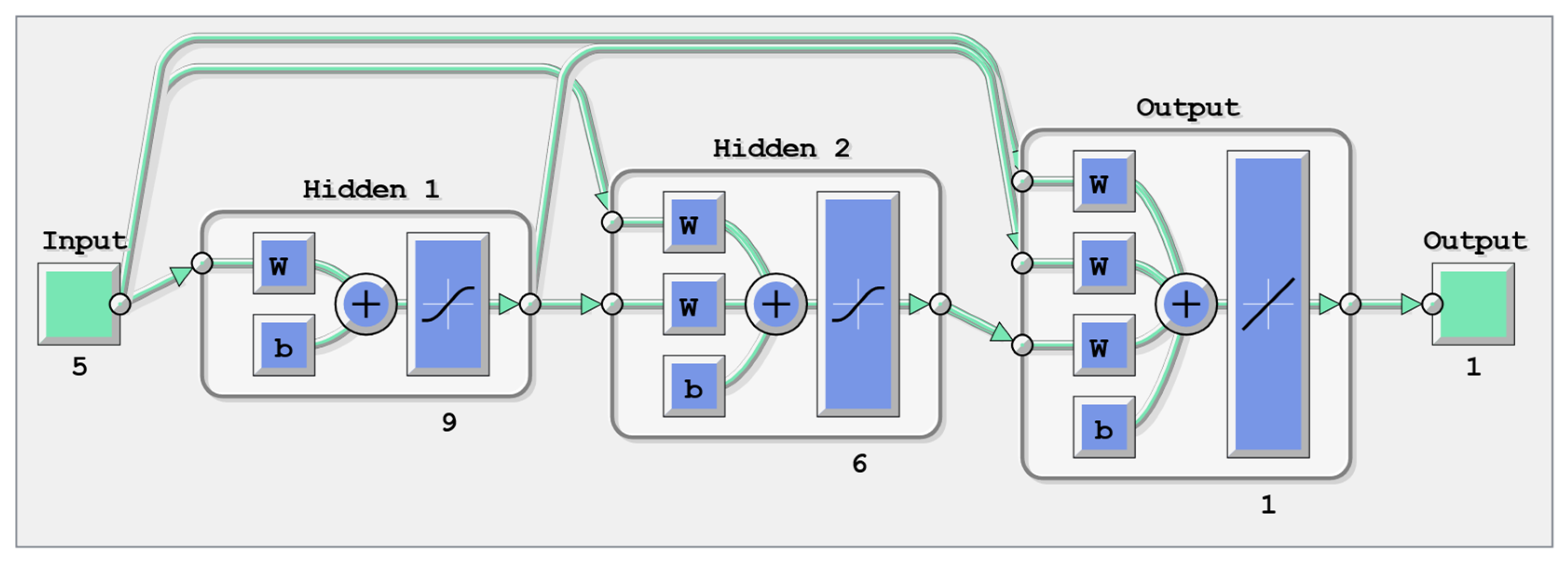
2.2. Artificial Neural Network Construction

The intention of this study was to widely screen the area of possible solutions, to find the most accurate. As the application of ANNs to model the performance of photovoltaic panels (PVs) is a novel approach, the evidence to exclude some of the possible configurations was very limited. Most studies use generic topologies. In this case, however, it was decided that a broader search should be conducted for higher prediction accuracy. Two ANN types were considered: feedforward and cascade forward [49]. The first is a simple system, where nodes are set linearly, without any connection to non-adjacent layers. The cascade forward ANN includes connections to the raw input and every previous layer to the following layers. The extra nonlinear relationship between input and output can improve accuracy in some scenarios, but on the other hand, can also lead to less predictable behavior of the system.

The next important aspect of the ANN is the selection of the training algorithm. Based on initial screening, eight algorithms were considered: BFGS Quasi-Newton, Resilient Backpropagation, Scaled Conjugate Gradient, Conjugate Gradient with Powell/Beale Restarts, Fletcher–Powell Conjugate Gradient, Polak–Ribiére Conjugate Gradient, One Step Secant, Variable Learning Rate Backpropagation. This very wide selection is intended to ensure that the algorithm will not bias a potentially good structure of the ANN. In the matter of performance function, four objective functions were tested: mean squared normalized error, mean absolute error, sum squared error, and sum absolute error.

2.3. Optimization Methodology and Meteorological Data Collection

As the number of optimized parameters is extraordinarily high and includes a different number of layers and the number of nodes inside the layers, only an automatic approach is feasible. In this study, a genetic algorithm (GA) was applied. This technique allows an efficient heuristic search for the global optimum (in this case the minimum) for a specific objective function. The exact form of the objective function, mean relative error (MRE), is presented below:

$$MRE=\frac{1}{n}·\left(\sum _{i=1}^n\frac{\left|P_T-P_{ANN}\right|}{P_T}\right)·100\%$$

(1)

where P_T denotes the target power output, measured on PV_S, and P_ANN refers to the output forecast by the network. The n value represents the number of measurements included in the sum. The maximal number of hidden layers was limited to 2, where the number of nodes could not exceed 10. Also, the proportions between the size of training, validation, and the test sample were constrained. The training set was assumed to have 80–95% of available measurements, the validation—5–20%, and the test—0–15%. The genetic algorithm was implemented in the MATLAB 2022b environment using the Global Optimization Toolbox package with a function tolerance of 1 × 10⁻² and a maximum number of generations limited to slightly over 50, based on previous screening. The GA was also constrained to ensure that the percentage of measurements selected for all three learning sets summed up to 100%.

Daily measurements of weather and the energy produced in 457 consecutive days were used as data for ANN learning. Days with zero production (maintenance or other disruptions) were excluded from the analysis. The input was meteorological information: maximal daily temperature (related to overheating of the PVs), sunshine duration (the most direct factor that defines the amount of energy produced), average cloud cover (common limiting factor), and time of precipitation (water on panels can decrease the efficiency in significant range). Additionally, to indirectly include information about the sun angle, the number of the day of the year was also included. This is an important aspect of novelty in this study, as this modification could not be applied to more conventional approaches. In typical modeling studies, only temporary factors are considered, while here, the most complex possible approach is applied.

3. Results and Discussion

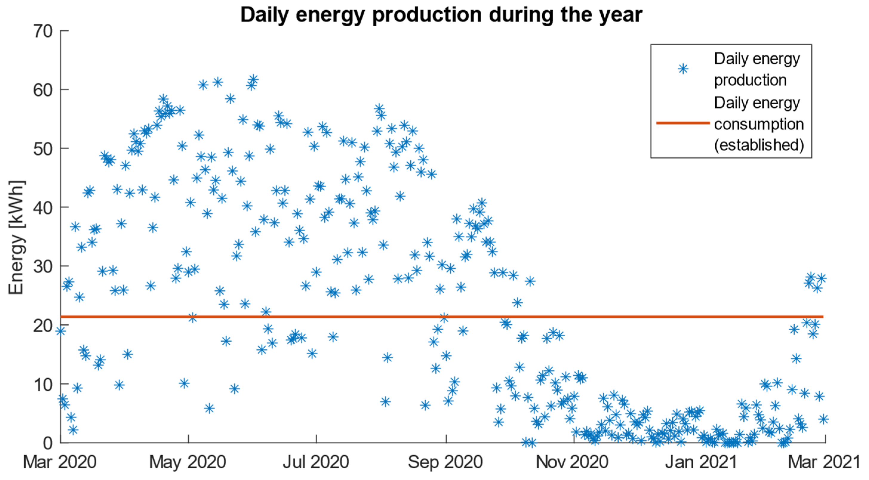
3.1. Annual Output of Tested Photovoltaic System

For all photovoltaic installations operating in the temperate zone, some relationship can be seen between the energy generated in summer and winter [50]. The course of daily energy consumption for the purpose of designing an installation adapted to the investor’s consumer needs was assumed to be constant. As can be seen from the below diagram, Figure 1, during the summer period, excess energy is generated and can be returned to the grid. The installation was intentionally slightly oversized. There was an overproduction of 766 kWh of energy per year. From the analyzed data, the year 2020 was quite unusual in terms of solar conditions in Poland. The highest amount of energy was produced in April. Usually, the sunniest month of the year is June or July, less often August or May. The 8.8 kWp installation produced more than 60 kWh of daily energy four times per year. The highest value was recorded on 1 June 2020 (61.714 kWh). From October to February, it was observed six times that the installation did not work during the day, and net energy production was zero due to weather conditions.

According to the manufacturer of the modules, solar radiation of $1000 \frac{\mathrm{W}}{{\mathrm{m}}^2}$ generates a current of 9.35 A and a voltage of 39.6 V. In order to reduce the influence of shading on individual cells, so-called power optimizers were installed at each module. A module produces a higher amount of energy if it operates at a higher power. This is highest when voltage and current values are high and very close to each other. The performance characteristics can be shown for a given amount of solar energy falling on the module. PV cells have been designed to operate under optimal conditions, which are considered to be rated conditions (in this case STC). As shown in Figure 2, the amount of generated power can be represented by a rectangle.

The area of the rectangle that is the ideal operating point is limited by the values of current and voltage. An ideal characteristic has been designated as a product of the voltage of the open circuit and the short circuit current of the solar cell [51]. The FF (fill factor) has the greatest value if it is defined as the ratio of an ideal characteristic to the point of maximum power. The FF corresponds to the voltage drop by the module during operation. The shadowing of parts of the module cells results in the flow of a much lower current and a shift of the operating point toward 0 [52]. The function of the optimizer is to find and enforce the work in the so-called maximum power point, allowing the system to work with the highest possible efficiency. For the analyzed case, the FF reached a value of 0.79. The results of the fill factor depend on the technology used and its durability. The operation of a photovoltaic panel with this efficiency is a satisfying result [53,54].

The device responsible for adapting the voltage and current to the requirements of the distribution network operator is the inverter. Due to this device, the generated energy can be transmitted to the grid and consumed by the prosumer at any time. The adaptation of the generated energy consists of changing the DC voltage to AC voltage with an effective value of 230 V (phase to neutral) and a frequency of 50 Hz. In addition, the inverter divides the voltage into 3 phases shifted by 120° and synchronizes them to the grid voltage. The used inverter has an efficiency as high as 99.5%.

According to the datasheet, the modules are very well adapted to exposure to external conditions. They have high protection class IP67, the tempered glass coating provides high impact and pressure resistance ($2400 \frac{\mathrm{N}}{{\mathrm{m}}^2})$, and the allowable operating temperature is within $\left(-40\right)–\left(+85\right)$ °C. The aluminum frame was attached to the structural members with bolted connections. The dimensions of a single module are 2008 × 1002 × 40 mm (about 2 ${\mathrm{m}}^2)$. A total of 144 photovoltaic cells were placed on its surface.

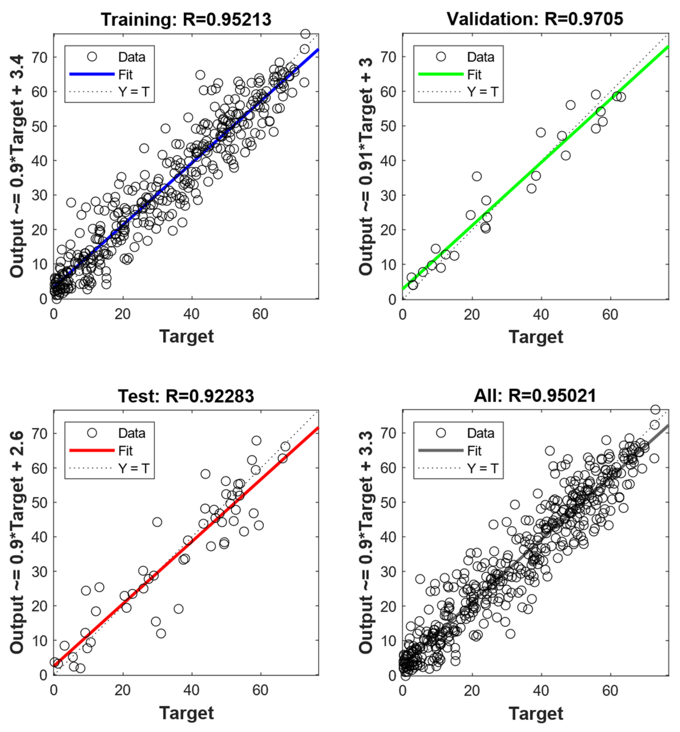
3.2. Optimization and Benchmarks of ANN

The primary tool used in this study to predict electricity production from panels was ANN. As mentioned in the Materials and Methods section, the GA was applied in this study to determine the best topology of the model (see Figure 3). The objective function for this procedure was the mean relative error of fitting between the ANN output and the measurement from the PVs. The relative error was selected, as it lets us adjust the actual differences by the size of the variable itself (see Section 2.2).

The GA required 51 generations (steps of calculation) to reach the minimum with the desired accuracy (function tolerance of 1 × 10⁻²). The progress of the GA is presented in Figure 3. As is noted, the penalty value shifted sharply during the procedure. The difference between best and worst in the selected generation reached above 30. However, the procedure stabilized in the last stage, after 43 generations, and any further changes did not improve the final score. The measured best, worst, and mean scores refer to all tested samples in the current generation and their objective function value.

Based on the calculations presented above, the final GA recommendation was as follows: the best accuracy was provided by the cascade forward ANN structure. The optimization algorithm had a lower impact on the final solution, with few exceptions. The resilient backpropagation procedure was found to be the best in the sense of the obtained accuracy (MRE) of the model. As the performance function for ANN learning, the best results were registered for sum squared error (SSE). The recommended size of the ANN was two hidden layers and one output layer. The hidden layers had nine and six nodes, respectively. Since the genetic algorithm is a heuristic and fully arbitrary tool, the resulting recommendation is solely based on the adopted goal function (MRE). The obtained optimal solution, therefore, is based on purely numerical considerations and is not based on an analytical evaluation of individual parameters. The visualization of the system is presented in Figure 4.

The distribution of available data between training, validation, and the test dataset was 82 to 6 to 12%. Splitting the data into subsets was a standard procedure to prevent false-positive model fits to experimental data. The higher size of test samples was found to be a good protection against overfitting. The results of the ANN training regression for the selected configuration were more than satisfactory. The overall R² value was 0.95, which indicates a very strong correlation. The best regression linearity (0.97) was achieved for the validation dataset—this can be explained by the fact that this subset was the smallest, so the result was in convergence with expectations. The lowest value was found for the test dataset (0.92). This set did not participate in the network’s training, so by design this result was to be expected. Nevertheless, how little the linearity of this set deviates from the other two proves that we are not dealing with overfitting, which is particularly important in this kind of research. The training dataset was in the middle, just around the mean value (see Figure 5). The linearity indices obtained should be considered very high compared with related studies where the obtained R² values, depending on weather conditions, were very close to those presented here [55].

To find the quantitative accuracy of the final model, as well as the GA objective function to distinguish it from ANN learning procedure objectives, the dataset from the last available 3 months was selected. Based on these data, a brief comparison between experimental and model values was performed. The final mean relative error (MRE) between the data set was 15.64%. The next comparison was intended to remove outliers. The points with an error greater than the mean value ± standard deviation were excluded, as they can be affected by objective problems resulting from the operating conditions in a normal outside environment. Only eight points fulfilled these conditions. After refining the dataset, a high improvement in accuracy was noted. The MRE was just 10.78%, which is a satisfying result given such diverse and general input data. Compared to other studies, it is possible to achieve even lower MRE values in the range of 4–5%, but mostly on synthetic data, which can be potentially more prone to interferences, while values from full forecasts rarely reach that low level of inaccuracy [56,57]. The visualization of raw, unrefined comparison between the experimental and ANN outputs is presented in Figure 6. It is also worth mentioning that the distribution of errors in the dataset was close to the normal distribution, with a slight shift toward positive values.

3.3. Case Study with ANN Application

To prove the practical potential of the created tool, a case study was performed. The intention of this part of the study was to show how the knowledge from the ANN forecast can be applied to optimize energy consumption and decrease the operational costs of the system, as well as minimize the environmental impact by achieving the highest share of renewable energy in the mix. In other words, the purpose of this chapter is to demonstrate the rationale behind the use of the model produced and the predictions it provides in optimizing the resources used. The following describes how using this tool can affect energy efficiency and reductions in external energy demand.

Three representative months were selected from available data—December, March, and May. In terms of PV project data, the first month represents the least sunny period of the year, the last month provides the most favorable conditions for PVs, while the middle one represents the intermediate season. The average monthly energy consumption assumed at the projecting stage of the PV installation was 641 kWh, and this value was assumed as a reference. To simplify calculations, the constant consumption per day was selected to be equal to 20.68 kWh. This value served as an unoptimized case, marked as “Constant” in Figure 7. The daily consumption in the ANN-optimized case was described using the following equation:

$$C_{opt}=AN{N}_{out}\ast \left(\frac{C_{month}}{{Sum}_{ANN}}\right)$$

(2)

where ANN_out describes the forecasted energy production for the selected day, C_month refers to the expected monthly energy consumption (641 kWh), and Sum_ANN describes the total sum of all ANN_our for the selected month. As a result, the energy consumption is automatically adjusted to match the C_month value at the end of the month. However, this strategy can be efficient only for months with a total production similar to or preferably higher than consumption. The visualization for March is presented in Figure 7 (see also Supplementary Materials Table S1).

As can be observed, the production covered the consumption for almost all days. The gap between these two values was only 11.96 kWh, which means that over 98.13% of the total monthly consumption can be supplied with PV production. Production was not sufficient to fully cover consumption in only 3 out of 31 days. For reference, the same calculation for constant energy consumption indicates only 84.25% of consumption coverage, which results in over 100 kWh that needs to be compensated by purchase from the power grid.

The difference between constant and optimized consumption is less pronounced for months with favorable conditions for energy production. In the case study for May, the unoptimized system covered 94.41% of the required energy, while the optimized system reached 98.90%. It is still significant and worth considering the benefits, but for months with high energy production, optimization is less important. For December, where the energy generated is lowest, both approaches give remarkably similar results—36.85% vs 36.74% for optimized and unoptimized cases, respectively. When the production is low in total, no numeric approach can overcome the physical limits of the system, and in both cases, energy needs to be bought from external sources, leading to negative installation income. Interesting results have been obtained from the economic analysis of both cases. To perform it, several assumptions have been made. First, an average price of 1 kWh was assumed at a level of 0.13€ based on current prices in the region of the study. The re-sell value is counted as 80% of the above-mentioned market price. In every case where production exceeded consumption, the profit equal to the sold energy was calculated. Alternatively, if the consumption exceeded production, the loss was measured. The emission was calculated following the recommendations of the National Center for Emissions Management and Balancing IOŚ-PIB (KOBiZE) in Poland, assuming a value of 719 kgCO₂/MWh [58]. A summary of the analysis is presented in

Table 1. Summary of economic analysis of case studies.

Month		March	May	December	Annual (Approximated)
Energy coverage (%)	Optimized	98.13	98.90	36.85	996.03
	Unoptimized	84.25	94.41	36.74	898.95
Installation gain (€)	Optimized	31.73	67.08	−52.18	235.08
	Unoptimized	29.42	66.34	−52.20	218.94
Emission reduction (kgCO2)	Optimized	452.26	455.81	169.83	4590.49
	Unoptimized	388.29	435.12	169.33	4143.07

. Cumulative values of energy coverage specified in Table 1 were defined by calculating the difference between energy usage and energy production. Thus, the final percentage was a summary of the final calculations using the modeled value of energy production versus the real energy production from measurements from the actual test plant. Installation gain describes the value of overproduced energy that can be sold at market rates, or in the case of negative values, the price that had to be paid to cover the cost of purchasing the missing power from the grid.

In the analysis, an approximated annual balance was calculated in addition to the three representative months. This was performed assuming that 3 months of the year are favorable for solar energy production, 3 are unfavorable, and 6 represent intermediate conditions:

$$Annual=I_{mar}·6+I_{may}·3+I_{dec}·3$$

(3)

This proportion was selected based on historical and prognosis data from the study of the tested PVs. The greatest benefits from energy consumption optimization based on the ANN can be seen in March. The balanced conditions give the widest area for the algorithm and allow for a reduction in external energy consumption by up to 16.47%. This results in an increase in installation gain of almost 8%. At the same time, CO₂ emission is reduced by 63.97 kg per month. Less pronounced improvements can also be noticed in May, with a 4.76% reduction in energy needed to be bought from the grid and 20.69 kg less CO₂ emitted. For December, the differences are negligible—under 0.6% for all the measured parameters.

Considering the improvements at the monthly scale, the gain can be considered moderate. However, if we calculate it annually, the conclusions change. The reduction in emissions at a level of 450 kg CO₂ per year cannot be omitted. The same can be said about the increase in the coverage of energy consumption by over 10%. Finally, it must be mentioned that the applied optimization method is very simple. Using more sophisticated methods could potentially allow one to obtain more from the data returned by the ANN.

4. Conclusions

The PV modules utilized in this study showed very high energy efficiency, but only in months with favorable conditions. This is a typical situation for temperate climates, as well as for most countries in the middle latitudes. The ANN is an efficient and precise method for predicting the output of PV systems in Poland. The proposed methodology, with an MRE of around 10.78%, is a good starting point for the optimization of energy generation and consumption and provides competitive accuracy compared with other similar works [55,56]. The case study indicated that the application of the ANN leads to a significant increase in profits (annually) and results in the reduction of CO₂ emission. The most significant benefits can be seen for months with moderate energy production. The ANN created in this study indicates significant advantages compared to similar approaches that can be found in the literature [57]. Besides typical parameters such as average daily solar irradiation, it also takes into account additional factors that affect the effectiveness of photovoltaic panels, such as ambient temperature, precipitation (water on PVs left over after rain muddies its works), or even the day of the year, as the latter indirectly carries information about the angle of the sun. The last aspect is especially uncommon compared with similar studies [59]. This allowed for modeling much more comprehensive and sensitive subtleties in the process.

References

1. Zimmermann, S.; Helmers, H.; Tiwari, M.K.; Paredes, S.; Michel, B.; Wiesenfarth, M.; Bett, A.W.; Poulikakos, D. A High-Efficiency Hybrid High-Concentration Photovoltaic System. Int. J. Heat Mass Transf. 2015, 89, 514–521. [Google Scholar] [CrossRef]
2. Raport Dotyczący Energii Elektrycznej Wytworzonej z OZE w Mikroinstalacji i Wprowadzonej Do Sieci Dystrybucyjnej (Art. 6a Ustawy o Odnawialnych Źródłach Energii); Polish Energy Regulatory Office: Warszawa, Poland, 2020.
3. EU Market Outlook for Solar Power 2021–2025—SolarPower Europe. Available online: https://www.solarpowereurope.org/insights/market-outlooks/market-outlook (accessed on 10 April 2022).
4. Directive (EU) 2018/2001 of the European Parliament and of the Council of 11 December 2018 on the Promotion of the Use of Energy from Renewable Sources (Text with EEA Relevance); EUR-Lex: Brussels, Belgium, 2018; Volume OJ L.
5. Renewable Power Generation Costs 2020; IRENA: Abu Dhabi, United Arab Emirates, 2021.
6. Wagner, A.; Matuszek, K.C. Time for Transition—Temporal Structures in Energy Governance in Contemporary Poland. Futures 2022, 140, 102959. [Google Scholar] [CrossRef]
7. Buriak, J. Ocena warunków nasłonecznienia i projektowanie elektrowni słonecznych z wykorzystaniem dedykowanego oprogramowania oraz baz danych. Zesz. Nauk. Wydziału Elektrotechniki I Autom. Politech. Gdańskiej 2014, Nr 40, 29–32. [Google Scholar]
8. IMGW. Raport IMGW-PIB: Klimat Polski 2020; IMGW: Warszawa, Poland, 2020. [Google Scholar]
9. Šúri, M.; Cebecauer, T.; Skoczek, A. SolarGIS: Solar Data And Online Applications For PV Planning And Performance Assessment. In Proceedings of the 26th European Photovoltaics Solar Energy Conference, Hamburg, Germany, 5–6 September 2011. [Google Scholar]
10. Oszacowanie Uzysku Energetycznego Systemu Fotowoltaicznego Estimation of Energy Yield of the PV System; Polskie Towarzystwo Fotowoltaiki: Warszawa, Poland, 2011.
11. Kardooni, R.; Yusoff, S.B.; Kari, F.B.; Moeenizadeh, L. Public Opinion on Renewable Energy Technologies and Climate Change in Peninsular Malaysia. Renew. Energy 2018, 116, 659–668. [Google Scholar] [CrossRef]
12. Zahurul, S.; Mariun, N.; Grozescu, I.V.; Tsuyoshi, H.; Mitani, Y.; Othman, M.L.; Hizam, H.; Abidin, I.Z. Future Strategic Plan Analysis for Integrating Distributed Renewable Generation to Smart Grid through Wireless Sensor Network: Malaysia Prospect. Renew. Sustain. Energy Rev. 2016, 53, 978–992. [Google Scholar] [CrossRef]
13. Abdullah, W.S.W.; Osman, M.; Ab Kadir, M.Z.A.; Verayiah, R. The Potential and Status of Renewable Energy Development in Malaysia. Energies 2019, 12, 2437. [Google Scholar] [CrossRef]
14. Energy Commission. Peninsular Malaysia Electricity Supply Outlook 2017; Suruhanjaya Tenaga: Putrajaya, Malaysia, 2017. [Google Scholar]
15. Figura, R.; Zientarski, W. Analiza parametrów pracy modułu fotowoltaicznego. Autobusy Tech. Eksploat. Syst. Transp. 2016, 17, 602–611. [Google Scholar]
16. Opiela, A.; Zapałowicz, Z. Uproszczony model wymiany energii w module PV z wymuszonym chłodzeniem powietrzem. Pol. Energetyka Słoneczna 2013, 1–4, 13–17. [Google Scholar]
17. Graham, V.A.; Hollands, K.G.T.; Unny, T.E. A Time Series Model for Kt with Application to Global Synthetic Weather Generation. Sol. Energy 1988, 40, 83–92. [Google Scholar] [CrossRef]
18. Duffie, J.A.; Beckman, W.A. Solar Engineering of Thermal Processes; Wiley: New York, NY, USA, 1991. [Google Scholar]
19. Erbs, D.G.; Klein, S.A.; Duffie, J.A. Estimation of the Diffuse Radiation Fraction for Hourly, Daily and Monthly-Average Global Radiation. Sol. Energy 1982, 28, 293–302. [Google Scholar] [CrossRef]
20. Demir, H. Simulation and Forecasting of Power by Energy Harvesting Method in Photovoltaic Panels Using Artificial Neural Network. Renew. Energy 2024, 222, 120017. [Google Scholar] [CrossRef]
21. Fouad, M.M.; Shihata, L.A.; Morgan, E.I. An Integrated Review of Factors Influencing the Perfomance of Photovoltaic Panels. Renew. Sustain. Energy Rev. 2017, 80, 1499–1511. [Google Scholar] [CrossRef]
22. Schinke-Nendza, A.; von Loeper, F.; Osinski, P.; Schaumann, P.; Schmidt, V.; Weber, C. Probabilistic Forecasting of Photovoltaic Power Supply—A Hybrid Approach Using D-Vine Copulas to Model Spatial Dependencies. Appl. Energy 2021, 304, 117599. [Google Scholar] [CrossRef]
23. Bounoua, Z.; Mechaqrane, A. Hourly and Sub-Hourly Ahead Global Horizontal Solar Irradiation Forecasting via a Novel Deep Learning Approach: A Case Study. Sustain. Mater. Technol. 2023, 36, e00599. [Google Scholar] [CrossRef]
24. Pereira, S.; Abreu, E.F.M.; Iakunin, M.; Cavaco, A.; Salgado, R.; Canhoto, P. Method for Solar Resource Assessment Using Numerical Weather Prediction and Artificial Neural Network Models Based on Typical Meteorological Data: Application to the South of Portugal. Sol. Energy 2022, 236, 225–238. [Google Scholar] [CrossRef]
25. Behrang, M.A.; Assareh, E.; Ghanbarzadeh, A.; Noghrehabadi, A.R. The Potential of Different Artificial Neural Network (ANN) Techniques in Daily Global Solar Radiation Modeling Based on Meteorological Data. Sol. Energy 2010, 84, 1468–1480. [Google Scholar] [CrossRef]
26. Al-Alawi, S.M.; Al-Hinai, H.A. An ANN-Based Approach for Predicting Global Radiation in Locations with No Direct Measurement Instrumentation. Renew. Energy 1998, 14, 199–204. [Google Scholar] [CrossRef]
27. Hassan, Q. Evaluation and Optimization of Off-Grid and on-Grid Photovoltaic Power System for Typical Household Electrification. Renew. Energy 2021, 164, 375–390. [Google Scholar] [CrossRef]
28. Fara, L.; Craciunescu, D. Output Analysis of Stand-Alone PV Systems: Modeling, Simulation and Control. Energy Procedia 2017, 112, 595–605. [Google Scholar] [CrossRef]
29. Ghimire, S.; Nguyen-Huy, T.; Deo, R.C.; Casillas-Pérez, D.; Salcedo-Sanz, S. Efficient Daily Solar Radiation Prediction with Deep Learning 4-Phase Convolutional Neural Network, Dual Stage Stacked Regression and Support Vector Machine CNN-REGST Hybrid Model. Sustain. Mater. Technol. 2022, 32, e00429. [Google Scholar] [CrossRef]
30. Khodadadi, M.; Sheikholeslami, M. Heat Transfer Efficiency and Electrical Performance Evaluation of Photovoltaic Unit under Influence of NEPCM. Int. J. Heat Mass Transf. 2022, 183, 122232. [Google Scholar] [CrossRef]
31. Karatepe, E.; Boztepe, M.; Colak, M. Neural Network Based Solar Cell Model. Energy Convers. Manag. 2006, 47, 1159–1178. [Google Scholar] [CrossRef]
32. Drałus, G.; Gomółka, Z. Prognozowanie produkcji energii elektrycznej w systemach fotowoltaicznych. Acta Sci. Acad. Ostroviensis Sect. A Nauk. Humanist. Społeczne I Tech. 2017, 9, 285–296. [Google Scholar]
33. Mellit, A.; Sağlam, S.; Kalogirou, S.A. Artificial Neural Network-Based Model for Estimating the Produced Power of a Photovoltaic Module. Renew. Energy 2013, 60, 71–78. [Google Scholar] [CrossRef]
34. Zheng, S.; Shahzad, M.; Asif, H.M.; Gao, J.; Muqeet, H.A. Advanced Optimizer for Maximum Power Point Tracking of Photovoltaic Systems in Smart Grid: A Roadmap towards Clean Energy Technologies. Renew. Energy 2023, 206, 1326–1335. [Google Scholar] [CrossRef]
35. Narasimman, K.; Gopalan, V.; Bakthavatsalam, A.K.; Elumalai, P.V.; Iqbal Shajahan, M.; Joe Michael, J. Modelling and Real Time Performance Evaluation of a 5 MW Grid-Connected Solar Photovoltaic Plant Using Different Artificial Neural Networks. Energy Convers. Manag. 2023, 279, 116767. [Google Scholar] [CrossRef]
36. Gaviria, J.F.; Narváez, G.; Guillen, C.; Giraldo, L.F.; Bressan, M. Machine Learning in Photovoltaic Systems: A Review. Renew. Energy 2022, 196, 298–318. [Google Scholar] [CrossRef]
37. Youssef, A.; El-Telbany, M.; Zekry, A. The Role of Artificial Intelligence in Photo-Voltaic Systems Design and Control: A Review. Renew. Sustain. Energy Rev. 2017, 78, 72–79. [Google Scholar] [CrossRef]
38. Postawa, K.; Fałtynowicz, H.; Pstrowska, K.; Szczygieł, J.; Kułażyński, M. Artificial Neural Networks to Differentiate the Composition and Pyrolysis Kinetics of Fresh and Long-Stored Maize. Bioresour. Technol. 2022, 364, 128137. [Google Scholar] [CrossRef] [PubMed]
39. Postawa, K.; Klimek, K.; Maj, G.; Kapłan, M.; Szczygieł, J. Advanced Dual-Artificial Neural Network System for Biomass Combustion Analysis and Emission Minimization. J. Environ. Manag. 2024, 349, 119543. [Google Scholar] [CrossRef] [PubMed]
40. Konjic, T.; Jahic, A.; Pihler, J. Artificial Neural Network Approach to Photovoltaic System Power Output Forecasting. In Proceedings of the 18th Intelligence Systems Applications to Power Systems ISAP 2015, Porto, Portugal, 11–16 September 2015. [Google Scholar]
41. Pelland, S.; Remund, J.; Kleissl, J.; Oozeki, T.; De Brabandere, K. Photovoltaic and Solar Forecasting: State of the Art; IEA PVPS 14; 2013; ISBN 978-3-906042-13-8. [Google Scholar]
42. Kleissl, J. Current State of the Art in Solar Forecasting; California Renewable Energy Forecasting, Resource Data and Mapping; University of California: San Francisco, CA, USA, 2013; p. 26. [Google Scholar]
43. Lo Brano, V.; Ciulla, G.; Di Falco, M. Artificial Neural Networks to Predict the Power Output of a PV Panel. Int. J. Photoenergy 2014, 2014, e193083. [Google Scholar] [CrossRef]
44. Shi, J.; Lee, W.-J.; Liu, Y.; Yang, Y.; Wang, P. Forecasting Power Output of Photovoltaic Systems Based on Weather Classification and Support Vector Machines. IEEE Trans. Ind. Appl. 2012, 48, 1064–1069. [Google Scholar] [CrossRef]
45. da Silva Fonseca, J.G., Jr.; Oozeki, T.; Takashima, T.; Koshimizu, G.; Uchida, Y.; Ogimoto, K. Use of Support Vector Regression and Numerically Predicted Cloudiness to Forecast Power Output of a Photovoltaic Power Plant in Kitakyushu, Japan. Prog. Photovolt. Res. Appl. 2012, 20, 874–882. [Google Scholar] [CrossRef]
46. Mandal, P.; Madhira, S.T.S.; Haque, A.U.; Meng, J.; Pineda, R.L. Forecasting Power Output of Solar Photovoltaic System Using Wavelet Transform and Artificial Intelligence Techniques. Procedia Comput. Sci. 2012, 12, 332–337. [Google Scholar] [CrossRef]
47. Saberian, A.; Hizam, H.; Radzi, M.A.M.; Ab Kadir, M.Z.A.; Mirzaei, M. Modelling and Prediction of Photovoltaic Power Output Using Artificial Neural Networks. Int. J. Photoenergy 2014, 2014, e469701. [Google Scholar] [CrossRef]
48. Krose, B.; van der Smagt, P. An Introduction to Neural Networks; University of Amsterdam: Amsterdam, The Netherlands, 1996. [Google Scholar]
49. Warsito, B.; Santoso, R.; Suparti; Yasin, H. Cascade Forward Neural Network for Time Series Prediction. J. Phys. Conf. Ser. 2018, 1025, 012097. [Google Scholar] [CrossRef]
50. Hastunç, M.; Karahüseyin, T.; Abbasoğlu, S. The Impact of COVID-19 Pandemic on the Electricity Production in Northern Cyprus under Increasing Installed Photovoltaic Capacity. Electr. Power Syst. Res. 2023, 215, 109023. [Google Scholar] [CrossRef]
51. Auf der Maur, M.; Di Carlo, A. Analytic Approximations for Solar Cell Open Circuit Voltage, Short Circuit Current and Fill Factor. Sol. Energy 2019, 187, 358–367. [Google Scholar] [CrossRef]
52. Belhachat, F.; Larbes, C. Global Maximum Power Point Tracking Based on ANFIS Approach for PV Array Configurations under Partial Shading Conditions. Renew. Sustain. Energy Rev. 2017, 77, 875–889. [Google Scholar] [CrossRef]
53. Obikoya, G.D.; Soman, A.; Das, U.K.; Hegedus, S.S. Investigation into Fill Factor and Open-Circuit Voltage Degradations in Silicon Heterojunction Solar Cells under Accelerated Life Testing at Elevated Temperatures. Sol. Energy Mater. Sol. Cells 2023, 263, 112586. [Google Scholar] [CrossRef]
54. Cheragee, S.H.; Alam, M.J. Device Modelling and Numerical Analysis of High-Efficiency Double Absorbers Solar Cells with Diverse Transport Layer Materials. Results Opt. 2024, 15, 100647. [Google Scholar] [CrossRef]
55. Miao, Y.; Lau, S.S.Y.; Lo, K.K.N.; Song, Y.; Lai, H.; Zhang, J.; Tao, Y.; Fan, Y. Harnessing Climate Variables for Predicting PV Power Output: A Backpropagation Neural Network Analysis in a Subtropical Climate Region. Sol. Energy 2023, 264, 111979. [Google Scholar] [CrossRef]
56. Hossain, M.S.; Mahmood, H. Short-Term Photovoltaic Power Forecasting Using an LSTM Neural Network and Synthetic Weather Forecast. IEEE Access 2020, 8, 172524–172533. [Google Scholar] [CrossRef]
57. López Gómez, J.; Ogando Martínez, A.; Troncoso Pastoriza, F.; Febrero Garrido, L.; Granada Álvarez, E.; Orosa García, J.A. Photovoltaic Power Prediction Using Artificial Neural Networks and Numerical Weather Data. Sustainability 2020, 12, 10295. [Google Scholar] [CrossRef]
58. KOBiZE. Wskaźniki Emisyjności CO2, SO2, NOx, CO i Pyłu Calkowitego Dla Energii Elektrycznej Grudzień 2020r. Available online: https://www.kobize.pl/uploads/materialy/materialy_do_pobrania/wskazniki_emisyjnosci/Wskazniki_emisyjnosci_grudzien_2020.pdf (accessed on 17 November 2021).
59. Villegas-Mier, C.G.; Rodriguez-Resendiz, J.; Álvarez-Alvarado, J.M.; Rodriguez-Resendiz, H.; Herrera-Navarro, A.M.; Rodríguez-Abreo, O. Artificial Neural Networks in MPPT Algorithms for Optimization of Photovoltaic Power Systems: A Review. Micromachines 2021, 12, 1260. [Google Scholar] [CrossRef] [PubMed]
Figure 1. Characteristics of annual electricity generation by a photovoltaic installation.
Applsci 14 02764 g001
Figure 2. Performance characteristics of the module for different solar irradiance values.
Applsci 14 02764 g002
Figure 3. The development of populations during the GA procedure.
Applsci 14 02764 g003
Figure 4. Visualization of the final ANN structure.
Applsci 14 02764 g004
Figure 5. The results of ANN training regression.
Applsci 14 02764 g005
Figure 6. Comparison between ANN and experimental data.
Applsci 14 02764 g006
Figure 7. Visualization of the case study for the month of March.
Applsci 14 02764 g007