Abstract
Due to the exceptional learning capabilities of deep neural networks (DNNs), they continue to struggle to handle label noise. To address this challenge, the pseudo-label approach has emerged as a preferred solution. Recent works have achieved significant improvements by exploring the information involved in DNN predictions and designing a straightforward method to incorporate model predictions into the training process by using a convex combination of original labels and predictions as the training targets. However, these methods overlook the feature-level information contained in the sample, which significantly impacts the accuracy of the pseudo label. This study introduces a straightforward yet potent technique named FPL (feature pseudo-label), which leverages information from model predictions as well as feature similarity. Additionally, we utilize an exponential moving average scheme to bolster the stability of corrected labels while upholding the stability of pseudo-labels. Extensive experiments were carried out on synthetic and real datasets across different noise types. The CIFAR10 dataset yielded the highest accuracy of 94.13% (Top1), while Clothing1M achieved 73.54%. The impressive outcomes showcased the efficacy and robustness of learning amid label noise.
1. Introduction
Deep learning relies on extensive datasets and has garnered significant achievements in domains like image classification [1], target detection [2], and image segmentation [3]. However, in real-world applications, annotating data can be prohibitively expensive. The quality of annotated samples might be compromised by subjective biases in manual labeling or tool limitations, resulting in label noise. The performance of DNNs in generalization frequently suffers when trained on datasets containing noisy labels. In real-world situations, training data are commonly gathered from various origins such as web searches [4] and crowdsourcing [5] in biased datasets. Consequently, effectively training DNNs with such noisy datasets poses a significant challenge within the realm of deep learning.
To tackle this challenge, numerous strategies have been suggested [6], falling into four primary categories. The initial strategy revolves around robust loss functions. While conventional loss functions such as cross-entropy (CE) [7] and mean squared error (MSE) [8] are sturdy, they may falter when dealing with intricate datasets. Hence, robust loss functions are formulated, incorporating supplementary steps and algorithms to enhance performance. The second strategy revolves around importance weighting, where smaller weights are allocated to potentially noisy samples while cleaner samples receive larger weights. This diminishes the impact of noisy labels on classification accuracy without entirely disregarding them. Moving to the third approach, loss correction operates under the assumption that noisy labels represent corrupted versions of clean labels, attributable to an unidentified noise transfer matrix. The objective of loss correction is to accurately learn this matrix to rectify the labels. Lastly, the fourth approach termed the pseudo-label method, is dedicated to rectifying identified dubious noisy labels to their accurate values. Unlike merely assigning higher weights to clean samples, the pseudo-label method delves into adjusting potentially incorrect labels. Typical pseudo-label techniques guide the training procedure toward the correct class by estimating the probability of rectifying the noise transfer matrix [9,10]. Alternatively, another approach entails employing the network to predict pseudo-labels for directly generated noisy labels, e.g., the approach proposed by Reed et al. [11] involves assigning a pseudo-label within the bootstrap loss, which constitutes a convex amalgamation of the original label and the predicted label, subsequently integrating it into the training regimen.
Although these techniques can produce pseudo-labels for noisy labels, the accuracy of such pseudo-labels might suffer if the classifier is inadequately trained. Additionally, these methods often overlook the impact of feature noise on classification performance. To tackle the aforementioned issues, this paper presents a method for generating feature labels from the feature layer to rectify the noisy labels. More precisely, we cluster the features extracted from the network, find the clustering center for each class, calculate its cosine similarity with each sample feature, and subsequently assign the feature labels based on the magnitude of the cosine similarity. Finally, we utilize a combination of the exponential moving average of pseudo-labels from the previous iteration, predicted labels, and feature labels to refine the accuracy of the pseudo-labels. The principal contributions of this study can be summarized as follows.
- •
- We introduce a simplified pseudo-labeling method that amalgamates the exponential moving average derived from the most recent round of pseudo-labels, predicted labels, and feature labels to form refined pseudo-labels. This approach is adept at handling datasets with differing noise types and levels.
- •
- We conducted thorough experiments on four benchmark datasets and one real dataset, covering four diverse noise types and two distinct noise levels. Our results consistently illustrate the superiority of our approach over prior methods, validating its efficacy.
2. Related Work
In this section, we aim to provide an overview of contemporary robust classification techniques tailored for addressing noisy labels. We will delve into prevalent methodologies concerning robustness loss functions, sample reweighting, and loss correction. Subsequently, our attention will transition towards examining pseudo-labeling methods.
A robust loss function ensures that the global minimum of the empirical risk minimization loss under clean labels possesses an equal probability of misclassification as the global minimum of the empirical risk minimization loss in a noisy dataset. For instance, the generalized cross-entropy (GCE) [12] integrates with the mean absolute error, and the inverse cross-entropy enhances the standard cross-entropy. Meanwhile, the symmetric cross-entropy (cross-entropy) [13] addresses under-learning and overfitting issues associated with noisy labels. The Taylor cross-entropy loss (TCE) [14] adjusts the fit of the training labels by controlling the order of the Taylor series. These methods have undergone extensive research and have demonstrated enhanced noise tolerance in the loss function. However, it has been observed that these effective loss functions may be susceptible to overfitting. To address this challenge, Ma et al. [15] proposed an active-passive loss (APL), which synergizes two mutually reinforced robust loss functions to attain heightened robustness and performance.
The alternate technique concerns the reweighting of samples, geared toward alleviating the influence of noisy labels on classification precision by allocating lower weights. A strategy embracing this concept is cooperative teaching (referenced as co-teaching) [16], which employs a collaborative teaching strategy to concurrently instruct two networks. Within this methodology, samples exhibiting lower loss are recognized as clean samples, and these specifically chosen samples are exchanged during training. FSR (fast sample reweighting) [17] is another method that addresses the sample reweighting problem without requiring an additional reward dataset. It resolves the issue of nested optimization models and the computationally expensive nature of second-order weighting parameters. MW-Net (meta-weight-net) [18] and CMW-Net [19] propose a meta-weighting network that circumvents the need for manually pre-setting hyperparameters, as is typically required in traditional sample weighting methods. These networks establish a mapping between loss functions and weights, enabling them to adaptively learn weighting functions directly from the data.
The third approach for tackling the label noise issue involves a method for correcting losses. A newly suggested approach is the noise transfer matrix method, which posits the presence of a probability matrix depicting the probability of a ground truth label transitioning into a noisy one. Patrini et al. [10] presented a loss correction method relying on a predictive forward or backward noise transfer matrix, derived from prior knowledge. However, without prior knowledge, the noise transfer matrix may not be effectively learned. Inspired by the traits of stochastic label corruption processes, Zhang et al. [20] suggested acquiring the noise transfer matrix from corrupted labels employing total variation regularization. Conversely, Wang et al. [21] employed meta-learning principles to introduce a novel meta-transformation learning approach, aimed at directly acquiring the noise transfer matrix from data within a meta-learning framework. This approach does not depend on prior knowledge to estimate the noise transfer matrix T. Instead, it directly optimizes T from the data, independent of any prior knowledge.
The primary objective of employing the pseudo-label method is to furnish model training with more precise labels. This is accomplished by correcting noisy labels to their accurate values through an extra inference step. Typically, certain pseudo-label methods leverage network predictions for noise rectification. For example, Hu et al. [22] obtained predictive distributions by augmenting samples with diverse strengths and weaknesses to produce corrected pseudo-labels. Another method proposed by Karim et al. [23] uses the average prediction of two different networks as corrected pseudo-labels. Moreover, there exists the potential for integrating meta-learning into labeling correction methods. Pham et al. [24] introduced a meta-pseudo-labeling method, which utilizes the teacher network to guide the student network. This involves generating pseudo-labels on unlabeled samples, with adjustments to the student’s performance on the labeled dataset made through feedback. Another approach is meta-label correction, where Wu et al. [25] and Zheng et al. [26] proposed meta-label correctors with different structures to map input labels to corrected soft labels without relying on traditional predefined generation rules, thus making the pseudo-labels generate process more flexible and adaptable to complex realistic datasets with different types and levels of noise.
This paper presents a method for addressing noisy samples at the feature level. We cluster these samples according to their extracted features to create pertinent feature labels. Our approach is independent of prior knowledge and does not solely rely on predicted labels as correction labels, avoiding potential oversight of crucial feature details.
3. Materials and Methods
Studying from noisy labels generally entails two data categories: modest datasets with clean labels and extensive datasets with noisy labels. Because manual labeling is both expensive and scarce, the quantity of samples for clean labeling is typically significantly less than those for noisy labeling. Nevertheless, exclusively training on a limited precise set and ignoring the image information encapsulated in the erroneous annotations compromises the robustness and adaptability of the DNNs, consequently resulting in a decrease in the overall training data volume. In response to these constraints, our proposition introduces a technique utilizing pseudo-labels. This approach facilitates amalgamating clean labels with pseudo-labels derived from rectified noisy labels throughout the learning phase. The methodology reconstructs the training annotations by applying an exponential moving average to the last round of corrected pseudo-labels, predicted labels, and feature labels. Throughout the training process, the noisy labels have the potential to be rectified over time, leading to an augmentation in the number of clean samples accessible for training purposes, consequently reducing the level of noise within the training dataset.
3.1. Preliminaries
DNNs typically consist of two primary components: the feature extractor, denoted as F, which processes input images and extracts their distinctive features, and the classifier, denoted as G, which generates classification probabilities based on the extracted image features provided by F. In the context of a K-class classification task, a dataset with noisy labels can be represented as , where N denotes the total number of samples in the dataset, represents the i-th sample, signifies the noisy labels, and C denotes the total number of classes. The feature extracted from the i-th sample by F is represented as , and the predicted labels for the i-th sample are denoted as .
Promoting the model to correct noise labels requires a direct strategy to minimize the cross-entropy loss between ground truth labels and prediction labels during the training phase. Specifically, for a sample, and its corresponding prediction, , the classifier, f, is updated throughout training iterations by minimizing the cross-entropy loss between and . This procedure can be described as follows:
In this context, n denotes the batch size, signifying the number of samples participating in the training process. Additionally, C symbolizes the total number of classes, with representing the individual element of the label for the i-th sample within the j-th class, and representing the corresponding element of the predicted label for the i-th sample within the j-th class.
3.2. Problems with Generating Pseudo-Labels
The research indicates that even when the training set is heavily corrupted, DNNs are capable of capturing and amplifying valuable information from noisy training data. Therefore, integrating the network’s predictions of training samples during the training phase for label correction can prove advantageous. The core pseudo-labeling approach entails utilizing a weighted average of the original label and the predicted label as the training objective, employing an exponential moving average mechanism denoted by . This exponential moving average mechanism helps alleviate the instability issue associated with model predictions and enables our algorithm to fully adapt the training labels when necessary, where , and . The corrected label, , is employed alongside the predicted label, , for computing the cross-entropy loss, and it can be expressed as follows:
However, during the initial phases of training, the model’s predictive accuracy might not reach a satisfactory level, leading to instability in the corrected labels. Additionally, in cases where the original label, , contains noise, the algorithm assigns a weight of to the actual predicted class. However, our ideal situation involves assigning full weight to the correct class label. Consequently, this approach could potentially impact the model’s classification accuracy.
3.3. Generate Feature Labels
To address the aforementioned issues, we suggest utilizing a blend of the exponential moving average of the previous round of pseudo-labels, predicted labels, and feature labels to generate corrected pseudo-labels at the feature level. The objective of this strategy is to address the instability observed in the corrected labels during the initial training phases and ensure that the ground-truth class labels are appropriately weighted, even when the original labels contain noise. Additionally, due to the incorporation of feature clustering in our algorithm, there may be a slight increase in computational time.
Initially, features, f, are extracted from all samples using the feature extractor, F. Given that the extracted features might vary in magnitude, we normalize the features based on their respective classes to obtain normalized features, .
This step is performed to facilitate the analysis of the raw feature data. We calculate the feature center, , for each class based on , as follows:
Here, c takes values from the set , denoting the specific class. C signifies the overall count of classes, while denotes the total samples, where ; this indicates the count of samples with a pseudo-label class, c. denotes the normalized feature of the i-th sample within the respective class.
In addition, to acquire feature labels, we compute the cosine similarity between each sample and the centroids of each feature class, denoted as .
where represents the corresponding class number. represents the cosine similarity between the i-th sample and the feature centroid, , of the j-th class.
Following this, we establish the feature label, , for each sample by evaluating its cosine similarity with the feature centers of each class. A greater cosine similarity suggests that the sample pertains to the class housing the respective feature center. Thus, we define the criterion as follows:
In this case, identifies the index of the highest value in a given set of operations. For example, if the value of is the highest, the returned value would be 3. In other words, would be equal to 3.
For each sample, we compute its cosine similarity to the centroid of each class. The higher the similarity to a centroid, the higher the probability of belonging to that class. By extracting features and calculating similarities, samples are assigned pseudo-labels based on the classification results, making the relationship between samples and their features more pronounced, extending beyond simple sample label predictions.
To rectify noisy labels for a larger sample set and render them viable, we employ pseudo-label updating. Through the utilization of an exponential moving average scheme, we progressively rectify noisy labels by model predictions and feature labels. This strategy aids in mitigating the volatility of model predictions, smooths the training process, and facilitates the complete overhaul of labels for training samples when necessary. In generating pseudo-labels, we extract features, f, from a small data batch and feed them into a classifier to derive predictions, p. Subsequently, the pseudo-labels, , are adjusted based on the prediction outcomes and feature labels:
Here, , , and are hyperparameters, with the constraint that . In the next section of the experiment, we will provide different hyperparameter settings for different datasets.
Based on the above, this paper also embraces a straightforward and efficient approach to sample reweighting. Defining the training target as , we set the weights, , as , and the sample weights, signify the confidence associated with the respective samples. Additionally, during the pre-training phase, all samples receive equal treatment. As the target undergoes updates, the FPL algorithm diminishes its focus on potentially noisy labels, shifting emphasis toward learning more from potentially clean samples. This strategy enables noisy samples to regain attention only if they can be confidently rectified.
Finally, the network’s parameters undergo updating via the cross-entropy loss computation between the predicted outcomes and the pseudo-labels assigned to the clean samples. This updating process can be expressed as follows:
Following the completion of training, we proceed to output and preserve the trained network model parameters. Algorithm 1 summarizes the essence of our proposed methodology. Additionally, as the DNNs initially adapt to the features of the clean labels, we initiate a warm-up phase. This warm-up phase enables the model to assimilate features that facilitate fine-tuning across various tasks, thereby improving the performance and accelerating the convergence of the model. Subsequently, we employ the proposed pseudo-label method to train the model.
| Algorithm 1: FPL |
|
4. Experiments and Discussion
To evaluate the effectiveness of our proposed approach, experiments were conducted on four benchmark datasets and one real dataset. We introduced different types of noise and varied noise rates, then proceeded to compare our findings with those obtained from existing learning techniques for handling noisy labels.
4.1. Experimental Setup
4.1.1. Datasets
Our proposed method was tested on simulated noisy datasets including SVHN [27], MNIST [28], CIFAR10, CIFAR100 [29], and one real dataset, Clothing1M [30]. SVHN is derived from real-world images featuring door numbers in Google Street View, encompassing 10 classes with images sized 32 × 32. It consists of 7325 images for training, 26,032 images for testing, and an additional 531,131 less challenging samples for training data. The MNIST handwritten digit dataset is a fundamental digital classification dataset, featuring 10 classes of grayscale images sized 28 × 28. It comprises 60k digital images for training and an additional 10,000 digital images for testing. CIFAR10 and CIFAR100 datasets are both composed of images sized 32 × 32, featuring 60k training images and 10k test images. The key distinction lies in the number of classes: CIFAR10 comprises 10 classes, whereas CIFAR100 encompasses 100 classes. Clothing1M comprises 14 classes of clothing images totaling 1M, sourced from various online shopping platforms, incorporating numerous mislabeled samples. Furthermore, the dataset comprises 50,000 training images, 14,000 validation images, and 10,000 testing images, all labels with accurate labels. Moreover, experiments were conducted on a noisy dataset with a long-tailed distribution [31], wherein the training data exhibited class imbalance following a long-tailed distribution pattern. To simulate this distribution, the quantity of training samples for various classes was reduced. Both the MNIST and SVHN datasets were employed for this setup. Furthermore, asymmetric noise was introduced to generate a noisy long-tailed dataset. Table 1 outlines the dataset details for all experiments conducted.

Table 1.
Dataset statistics and classifier architectures used.
4.1.2. Noise Types
We conducted multiple experiments with various noise rates and types. While Clothing1M, being a real dataset, possessed naturally occurring noisy labels, no supplementary noise was artificially introduced. Conversely, for MNIST, SVHN, CIFAR10, and CIFAR100, label corruption was deliberately induced using four different types of noise: symmetric noise, pair flip noise, tridiagonal noise, and instance noise. The composition of these different noise types is detailed as follows:
- 1.
- Symmetric noise: All samples have an equal probability of being mislabeled as other samples. This approach follows the method described by Zhang et al. [32] and Tanaka et al. [33].
- 2.
- Pair flip noise: Acquiring the pristine labels within each category involves randomly flipping to adjacent classes with equal likelihood.
- 3.
- Tridiagonal noise: This type of noise is created by performing two consecutive pairwise flips of two classes in opposite directions.
- 4.
- Instance noise: The likelihood of an object receiving an erroneous label depends on its attributes or properties.
4.1.3. Baselines
This paper utilizes the original code version and default configurations; this study reproduces the state-of-the-art technique and subsequently contrasts its performance against FPL.
- 1.
- GCE [12]: A novel GCE loss function integrates the robustness to noise characteristic of the mean absolute error (MAE) loss function with the training expediency inherent in the conventional cross-entropy loss function.
- 2.
- APL [15]: A framework is suggested for crafting a robust loss function, termed active passive loss (APL). APL synergizes two interdependent robust loss functions to enhance both robustness and performance.
- 3.
- ELR [34]: Takes advantage of early learning through regularization. Firstly, the semi-supervised learning technique is used to generate the target probability according to the model output. Secondly, a regularization term is designed to guide the model to these targets, implicitly preventing the memory of false labels.
- 4.
- CDR [35]: This method categorizes parameters into critical and non-critical, employing distinct update regulations for various parameter types.
- 5.
- MSLC: Introduces a meta-learning model designed to predict soft labels by implementing a meta-gradient descent procedure guided by clean metadata, thereby efficiently allocating pseudo-labels to noisy ones.
- 6.
- PES [36]: Trains the network into different parts to counteract the effects of label noise.
- 7.
- MLC: The label correction process is considered a meta-process, where the label correction network functions as a meta-model to generate corrected pseudo-labels for noisy labels. Concurrently, the main model is trained to learn from these pseudo-labels instead of the noisy labels. Introduces a fresh contrast regularization function for acquiring representations in the presence of noisy data, mitigating the influence of label noise.
- 8.
- CTRR [37]: Proposes a new contrast regularization function for acquiring representations in the presence of noisy data, relieving the influence of label noise.
4.1.4. Network Structure
To ensure fairness, we implemented all methods using PyTorch with default parameters. All experiments were conducted on Nvidia Tesla RTX3090 GPUs (Nvidia, Santa Clara, CA, USA). For the MNIST dataset, we used a 9-layer CNN. For the SVHN, CIFAR10, and CIFAR100 datasets, we used the ResNet34 network structure. For the Clothing1M dataset, we used the ResNet18 network structure.
In our experiments on SVHN, MNIST, CIFAR10, and CIFAR100 datasets, we employed the Adam optimizer with a momentum of 0.9. The initial learning rate was fixed at 0.001, and the batch size was set to 128. Models were trained for 200 epochs on each dataset. The implementation details for the long-tail dataset were aligned with those of the experiments conducted on the balanced noise dataset.
For the Clothing1M experiments, we utilized the Adam optimizer with a momentum of 0.9 and set the batch size to 64. Throughout the training phase, we completed a total of 15 epochs. The learning rate was set to for the first 5 epochs, followed by for the next 5 epochs, and finally for the remaining 5 epochs.
4.1.5. Parameter Analysis
, , and , respectively, represent the confidence proportion of the last round of pseudo-labels after the update, the confidence proportion of the prediction labels after the update, and the confidence proportion of the feature labels after the update. According to the concept of exponential moving average, the sum of these three parameters should equal 1. When the confidence of prediction labels and feature labels is high, the updated pseudo-labels will overly rely on the overall model performance, increasing the risk of overfitting in later training stages. In most scenarios, aside from the original clean labels, there is no guarantee that the corrected pseudo-labels are accurate, underscoring the critical importance of setting these three parameters thoughtfully. In this section, we will set three sets of hyperparameters, namely , , ; , , ; and , , . Experiments were performed on the CIFAR100 dataset, and the results of the experiments are shown in Table 2.
Table 2.
Average test accuracy (%) for the last 10 epochs with different hyperparameter settings on CIFAR100. The best mean results are in bold.
According to the experimental findings, the highest test accuracy across the four noise types is achieved when setting the parameters to , , and . Due to the vast number of classes in CIFAR100, the classifier requirements are relatively stricter compared to other datasets, increasing the chance of feature learning errors. Hence, a decreased ratio of coefficients associated with feature labels proves advantageous. However, a lack of fine-tuning based on feature labeling can likewise lead to lower test accuracy.
Based on the experimental settings mentioned above, we established the particular parameter configurations for four baseline datasets and one real dataset, respectively. For the MNIST dataset, we set , , and for all four noise types. For the SVHN dataset, we set , , and . For the CIFAR10 dataset, we used the same parameter settings for symmetric noise, pair flip noise, and tridiagonal noise, which were , , and . For instance noise on CIFAR10, we set , , and . For the CIFAR100 dataset, we set , , and . For the Clothing1M dataset, we used the parameter settings of , , and for all four noise types. Finally, for both im-SVHN and im-MNIST datasets, we used the same parameter settings of , , and for all four noise types. To provide a clearer representation, we organized the specific parameters in a table format. Please refer to Table 3 for detailed information.
Table 3.
The settings of three parameters for different noise types in different datasets.
4.2. Results and Discussion
4.2.1. Results on Simulated Noise Datasets
The average test accuracies of the last ten epochs for FPL and all baseline algorithms across eight different settings are presented in Table 4. Regarding MNIST, SVHN, and CIFAR10 datasets, the method proposed in this paper demonstrates a clear advantage over all other comparison experiments. Moreover, the class accuracy is close to 100% on the MNIST dataset, indicating the method’s effectiveness for MNIST. Additionally, for the CIFAR10 dataset, the algorithm exhibits a significant advantage over the CTRR algorithm in the case of Instance-40%, with a nearly 2% higher performance, suggesting that the FPL algorithm performs well in scenarios involving Instance noise associated with image features. For the pair flip-20%, the accuracy of the CIFAR100 dataset is lower compared to that of the ELR algorithm. ELR, unlike FPL, does not directly correct the noisy labels but instead hinders the model from memorizing them by incorporating a specially crafted regularization term. Although both are in the field of label noise, these methods approach the problem differently, resulting in different performances for different noise types. Furthermore, the ELR approach only marginally outperforms FPL by 0.03%, leaving room for chance factors to influence results. Besides, the FPL method demonstrates a smaller difference between high and low noise rates compared to other methods in similar noise types. For instance, the disparity between the 40% noise rate and the 20% noise rate under the pair flip noise type is 1.08%, while the difference for the ELR method is 1.77%. These results demonstrate that FPL yields better classification results at higher noise rates. In summary, the method exhibits good convergence and stability across the four benchmark datasets. Additionally, the FPL algorithm demonstrates a relatively small range of standard deviation variation in the last 10 epochs, further indicating the robustness of the algorithm.
Table 4.
Average test accuracy (%) on four simulated noise datasets over the last 10 epochs. The best mean results are in bold.
4.2.2. Results on Real Datasets
The best and final results of the FPL for the Clothing1M dataset are presented in Table 5. As it is a real dataset with labeling noise, there is no need to artificially introduce additional noise. In contrast to other baseline methods, although this approach may not attain the highest classification accuracy in terms of optimal results, the FPL method demonstrates the highest classification accuracy at the last epoch. The difference between the best and final outcomes of the FPL algorithm indicates robust stability and exceptional convergence on real datasets.
Table 5.
Test accuracy (%) on Clothing1M. The best mean results are in bold.
4.2.3. Results on Imbalance Datasets
We assessed the performance of our model on noisy long-tailed number datasets featuring four different noise rates. In contrast to other algorithms, the approach presented in this paper displays a distinct advantage regarding classification accuracy. Moreover, compared to alternative algorithms, our method showcases superior convergence, evident from consistently smaller variances during the last 10 epochs. These observations indicate the competitiveness of our approach. Experimental results for the imbalanced MNIST dataset are presented in Table 6, while those for the imbalanced SVHN dataset are showcased in Table 7.
Table 6.
Average test accuracy (%) on im-MNIST over the last 10 epochs. The best mean results are in bold.
Table 7.
Average test accuracy (%) on im-SVHN over the last 10 epochs. The best mean results are in bold.
4.3. Ablation Experiments
To evaluate the effectiveness of feature labels and predictive labels, we conducted ablation experiments. The settings and outcomes of the ablation experiment on the CIFAR10 dataset can be found in Table 8. All models employed in these experiments were derived from the ResNet architecture.
Table 8.
Average test accuracy (%) of the ablation experiment on CIFAR10. The best mean results are in bold. “P” represents the prediction label, “F” represents the feature label and “” represents which module to apply.
The test accuracy of CIFAR10 across different epochs is depicted in Figure 1. In the majority of experimental settings, the test accuracy is lower when the feature tag is not utilized compared to when it is employed. For Instance-20%, the classification accuracy is merely 0.02% higher than that of the FPL algorithm, which may be influenced by incidental factors. In the scenario of Tridiagonal-20%, the impact of solely incorporating prediction labels is notably more pronounced. Therefore, enhancements are required for the FPL algorithm in this type of noise. Nonetheless, we also computed the average classification accuracy for each ablation experiment configuration, revealing that our method consistently attained significant advantages in average accuracy. Moreover, the method without predicted labels exhibits a noticeable decline after 30 epochs, whereas our method remains more stable. This pattern is especially conspicuous when confronted with higher noise rates, suggesting that our proposed method excels under such circumstances.
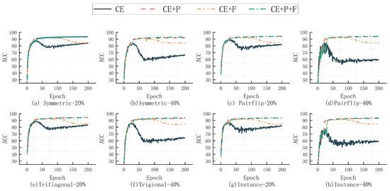
Figure 1.
Ablation experiments on CIFAR10.
4.4. Experimental Complexity Evaluation
The FPL algorithm’s superiority is emphasized by using training time as a criterion for evaluating the experiment’s complexity. We applied a symmetric noise setting to the CIFAR10 dataset, with a noise rate of 20%. Each comparison method underwent 200 training sessions under identical experimental conditions. Furthermore, to underscore the duration of the feature clustering process, we conducted supplementary experiments devoid of feature labels, designated as FPL (w/o), and their outcomes are displayed in Table 9. Upon reviewing the table, it becomes apparent that our proposed method demonstrates a reduced runtime compared to alternative benchmark algorithms, notably surpassing the performance of the MLC and MSLC pseudo-labeling techniques. This implies that our approach attains superior classification accuracy while retaining lower complexity. Furthermore, we noted a mere 0.73 h reduction in training time after removing the feature labels. This suggests that the feature clustering process has minimal impact on the overall complexity of the training cycle.
Table 9.
Comparison of running times on the CIFAR10 dataset. The shortest running time is in bold.
5. Conclusions
This paper presents a novel pseudo-label approach aimed at bolstering the robustness of DNNs in the presence of noisy labels. The core concept involves leveraging feature clustering to compute cosine similarity, facilitating the acquisition of precise feature labels for rectifying noisy labels. Our experimentation spanned multiple datasets, encompassing MNIST, SVHN, CIFAR10, CIFAR100, and Clothing1M. The findings illustrate the superior performance of our method, especially under high noise rate conditions. Furthermore, we conducted ablation experiments to affirm the efficacy of our proposed feature labels.
Author Contributions
Writing—original draft, X.W.; Writing—review & editing, Z.W.; Supervision, P.W.; Funding acquisition, Y.D. All authors have read and agreed to the published version of the manuscript.
Funding
This research was funded by National Natural Science Foundation of China grant number 62306103.
Institutional Review Board Statement
Not applicable.
Informed Consent Statement
Not applicable.
Data Availability Statement
The original contributions presented in the study are included in the article, further inquiries can be directed to the corresponding author.
Conflicts of Interest
The authors declare no conflicts of interest.
References
- Krizhevsky, A.; Sutskever, I.; Hinton, G.E. Imagenet classification with deep convolutional neural networks. Commun. ACM 2017, 60, 84–90. [Google Scholar] [CrossRef]
- Girshick, R.; Donahue, J.; Darrell, T.; Malik, J. Rich feature hierarchies for accurate object detection and semantic segmentation. In Proceedings of the IEEE Conference on Computer Vision and Pattern Recognition, Columbus, OH, USA, 23–28 June 2014; pp. 580–587. [Google Scholar]
- Chen, L.C.; Papandreou, G.; Kokkinos, I.; Murphy, K.; Yuille, A.L. Deeplab: Semantic image segmentation with deep convolutional nets, atrous convolution, and fully connected crfs. IEEE Trans. Pattern Anal. Mach. Intell. 2017, 40, 834–848. [Google Scholar] [CrossRef] [PubMed]
- Liu, W.; Jiang, Y.G.; Luo, J.; Chang, S.F. Noise resistant graph ranking for improved web image search. In Proceedings of the CVPR 2011, Colorado Springs, CO, USA, 20–25 June 2011; pp. 849–856. [Google Scholar]
- Welinder, P.; Branson, S.; Perona, P.; Belongie, S. The multidimensional wisdom of crowds. In Proceedings of the Advances in Neural Information Processing Systems, Vancouver, BC, Canada, 6–9 December 2010; Volume 23. [Google Scholar]
- Song, H.; Kim, M.; Park, D.; Shin, Y.; Lee, J.G. Learning from noisy labels with deep neural networks: A survey. IEEE Trans. Neural Netw. Learn. Syst. 2022, 34, 8135–8153. [Google Scholar] [CrossRef] [PubMed]
- Wang, Y.; Liu, W.; Ma, X.; Bailey, J.; Zha, H.; Song, L.; Xia, S.T. Iterative learning with open-set noisy labels. In Proceedings of the IEEE Conference on Computer Vision and Pattern Recognition, Salt Lake City, UT, USA, 18–23 June 2018; pp. 8688–8696. [Google Scholar]
- Ghosh, A.; Kumar, H.; Sastry, P.S. Robust loss functions under label noise for deep neural networks. In Proceedings of the AAAI Conference on Artificial Intelligence, San Francisco, CA, USA, 4–9 February 2017; Volume 31. [Google Scholar]
- Hendrycks, D.; Mazeika, M.; Wilson, D.; Gimpel, K. Using trusted data to train deep networks on labels corrupted by severe noise. In Proceedings of the Advances in Neural Information Processing Systems, Montréal, QC, Canada, 3–8 December 2018; Volume 31. [Google Scholar]
- Patrini, G.; Rozza, A.; Krishna Menon, A.; Nock, R.; Qu, L. Making deep neural networks robust to label noise: A loss correction approach. In Proceedings of the IEEE Conference on Computer Vision and Pattern Recognition, Honolulu, HI, USA, 21–26 July 2017; pp. 1944–1952. [Google Scholar]
- Reed, S.; Lee, H.; Anguelov, D.; Szegedy, C.; Erhan, D.; Rabinovich, A. Training deep neural networks on noisy labels with bootstrapping. arXiv 2014, arXiv:1412.6596. [Google Scholar]
- Zhang, Z.; Sabuncu, M. Generalized cross entropy loss for training deep neural networks with noisy labels. In Proceedings of the Advances in Neural Information Processing Systems, Montréal, QC, Canada, 3–8 December 2018; Volume 31. [Google Scholar]
- Wang, Y.; Ma, X.; Chen, Z.; Luo, Y.; Yi, J.; Bailey, J. Symmetric cross entropy for robust learning with noisy labels. In Proceedings of the IEEE/CVF International Conference on Computer Vision, Seoul, Republic of Korea, 27 October–2 November 2019; pp. 322–330. [Google Scholar]
- Feng, L.; Shu, S.; Lin, Z.; Lv, F.; Li, L.; An, B. Can cross entropy loss be robust to label noise? In Proceedings of the Twenty-Ninth International Conference on International Joint Conferences on Artificial Intelligence, Online, 7–15 January 2021; pp. 2206–2212. [Google Scholar]
- Ma, X.; Huang, H.; Wang, Y.; Romano, S.; Erfani, S.; Bailey, J. Normalized loss functions for deep learning with noisy labels. In Proceedings of the International Conference on Machine Learning, PMLR, Virtual Event, 13–18 July 2020; pp. 6543–6553. [Google Scholar]
- Han, B.; Yao, Q.; Yu, X.; Niu, G.; Xu, M.; Hu, W.; Tsang, I.; Sugiyama, M. Co-teaching: Robust training of deep neural networks with extremely noisy labels. In Proceedings of the Advances in Neural Information Processing Systems, Montréal, QC, Canada, 3–8 December 2018; Volume 31. [Google Scholar]
- Zhang, Z.; Pfister, T. Learning fast sample re-weighting without reward data. In Proceedings of the IEEE/CVF International Conference on Computer Vision, Virtual, 11–17 October 2021; pp. 725–734. [Google Scholar]
- Shu, J.; Xie, Q.; Yi, L.; Zhao, Q.; Zhou, S.; Xu, Z.; Meng, D. Meta-weight-net: Learning an explicit mapping for sample weighting. In Proceedings of the Advances in Neural Information Processing Systems, Vancouver, BC, Canada, 8–14 December 2019; Volume 32. [Google Scholar]
- Shu, J.; Yuan, X.; Meng, D.; Xu, Z. CMW-Net: Learning a class-aware sample weighting mapping for robust deep learning. arXiv 2022, arXiv:2202.05613. [Google Scholar] [CrossRef] [PubMed]
- Zhang, Y.; Niu, G.; Sugiyama, M. Learning noise transition matrix from only noisy labels via total variation regularization. In Proceedings of the International Conference on Machine Learning, PMLR, Virtual Event, 28–24 July 2021; pp. 12501–12512. [Google Scholar]
- Wang, Z.; Hu, G.; Hu, Q. Training noise-robust deep neural networks via meta-learning. In Proceedings of the IEEE/CVF Conference on Computer Vision and Pattern Recognition, Seattle, WA, USA, 13–19 June 2020; pp. 4524–4533. [Google Scholar]
- Hu, Z.; Yang, Z.; Hu, X.; Nevatia, R. Simple: Similar pseudo label exploitation for semi-supervised classification. In Proceedings of the IEEE/CVF Conference on Computer Vision and Pattern Recognition, Nashville, TN, USA, 20–25 June 2021; pp. 15099–15108. [Google Scholar]
- Karim, N.; Rizve, M.N.; Rahnavard, N.; Mian, A.; Shah, M. Unicon: Combating label noise through uniform selection and contrastive learning. In Proceedings of the IEEE/CVF Conference on Computer Vision and Pattern Recognition, New Orleans, LA, USA, 18–24 June 2022; pp. 9676–9686. [Google Scholar]
- Pham, H.; Dai, Z.; Xie, Q.; Le, Q.V. Meta pseudo labels. In Proceedings of the IEEE/CVF Conference on Computer Vision and Pattern Recognition, Nashville, TN, USA, 20–25 June 2021; pp. 11557–11568. [Google Scholar]
- Wu, Y.; Shu, J.; Xie, Q.; Zhao, Q.; Meng, D. Learning to purify noisy labels via meta soft label corrector. In Proceedings of the AAAI Conference on Artificial Intelligence, Virtually, 2–9 February 2021; Volume 35, pp. 10388–10396. [Google Scholar]
- Zheng, G.; Awadallah, A.H.; Dumais, S. Meta label correction for noisy label learning. In Proceedings of the AAAI Conference on Artificial Intelligence, Virtually, 2–9 February 2021; Volume 35, pp. 11053–11061. [Google Scholar]
- Netzer, Y.; Wang, T.; Coates, A.; Bissacco, A.; Wu, B.; Ng, A.Y. Reading digits in natural images with unsupervised feature learning. NIPS Workshop Deep. Learn. Unsupervised Feature Learn. 2011, 2011, 7. [Google Scholar]
- Deng, L. The mnist database of handwritten digit images for machine learning research [best of the web]. IEEE Signal Process. Mag. 2012, 29, 141–142. [Google Scholar] [CrossRef]
- Krizhevsky, A.; Hinton, G. Learning multiple layers of features from tiny images. Handb. Syst. Autoimmune Dis. 2009, 1. [Google Scholar]
- Xiao, T.; Xia, T.; Yang, Y.; Huang, C.; Wang, X. Learning from massive noisy labeled data for image classification. In Proceedings of the IEEE Conference on Computer Vision and Pattern Recognition, Boston, MA, USA, 7–12 June 2015; pp. 2691–2699. [Google Scholar]
- Yang, Y.; Xu, Z. Rethinking the value of labels for improving class-imbalanced learning. Adv. Neural Inf. Process. Syst. 2020, 33, 19290–19301. [Google Scholar]
- Zhang, C.; Bengio, S.; Hardt, M.; Recht, B.; Vinyals, O. Understanding deep learning (still) requires rethinking generalization. Commun. ACM 2021, 64, 107–115. [Google Scholar] [CrossRef]
- Tanaka, D.; Ikami, D.; Yamasaki, T.; Aizawa, K. Joint optimization framework for learning with noisy labels. In Proceedings of the IEEE Conference on Computer Vision and Pattern Recognition, Salt Lake City, UT, USA, 18–23 June 2018; pp. 5552–5560. [Google Scholar]
- Liu, S.; Niles-Weed, J.; Razavian, N.; Fernandez-Granda, C. Early-learning regularization prevents memorization of noisy labels. Adv. Neural Inf. Process. Syst. 2020, 33, 20331–20342. [Google Scholar]
- Xia, X.; Liu, T.; Han, B.; Gong, C.; Wang, N.; Ge, Z.; Chang, Y. Robust early-learning: Hindering the memorization of noisy labels. In Proceedings of the International Conference on Learning Representations, Vienna, Austria, 3–7 May 2021. [Google Scholar]
- Bai, Y.; Yang, E.; Han, B.; Yang, Y.; Li, J.; Mao, Y.; Niu, G.; Liu, T. Understanding and improving early stopping for learning with noisy labels. Adv. Neural Inf. Process. Syst. 2021, 34, 24392–24403. [Google Scholar]
- Yi, L.; Liu, S.; She, Q.; McLeod, A.I.; Wang, B. On learning contrastive representations for learning with noisy labels. In Proceedings of the IEEE/CVF Conference on Computer Vision and Pattern Recognition, New Orleans, LA, USA, 18–24 June 2022; pp. 16682–16691. [Google Scholar]
Disclaimer/Publisher’s Note: The statements, opinions and data contained in all publications are solely those of the individual author(s) and contributor(s) and not of MDPI and/or the editor(s). MDPI and/or the editor(s) disclaim responsibility for any injury to people or property resulting from any ideas, methods, instructions or products referred to in the content. |
© 2024 by the authors. Licensee MDPI, Basel, Switzerland. This article is an open access article distributed under the terms and conditions of the Creative Commons Attribution (CC BY) license (https://creativecommons.org/licenses/by/4.0/).