Research on the Processing of Image and Spectral Information in an Infrared Polarization Snapshot Spectral Imaging System

Abstract

In order to solve the problems of a low target recognition rate and poor real-time performance brought about by conventional infrared imaging spectral detection technology under complex background conditions or in the detection of targets of weak radiation or long distance, a kind of infrared polarization snapshot spectral imaging system (PSIFTIS) and a spectrum information processing method based on micro-optical devices are proposed in this paper, where the synchronous acquisition of polarization spectrum information is realized through the spatial modulation of phase with a rooftop-shaped multi-stage micro-mirror and the modulation of the polarization state of light with a micro-nanowire array. For the polarization interference image information obtained, the infrared polarization spectrum decoupling is realized by image segmentation, optical path difference matching, and image registration methods, the infrared polarization spectrum reconstruction is realized by Fourier transform spectral demodulation, and the infrared polarization image fusion is realized by decomposing and reconstructing the high- and low-frequency components of the polarization image based on the Haar wavelet transform. The maximum spectral peak wavenumber error of the four polarization channels of the polarization spectrum reconstruction is less than 2 cm⁻¹, and the polarization angle error is within 1°. Ultimately, compared with the unprocessed polarization image unit, the peak signal-to-noise ratio is improved by 45.67%, the average gradient is improved by 8.03%, and the information entropy is improved by 56.98%.

1. Introduction

With the rapid development of aerospace remote sensing, resource surveys, medical biology, military reconnaissance, agriculture, and other fields, there is an urgent need for high-performance infrared imaging detection instruments, and higher requirements have been put forward for the real-time detection of transient targets, weak signal detection ability, compact structure, and stability. The multidimensional information acquisition technology developed on the basis of infrared imaging spectroscopy and polarization imaging technology, known as infrared polarization spectroscopy imaging technology, has unique advantages. It can obtain the imaging, spectral, and polarization information of the detected target at the same time, greatly improving the amount of information obtained by optical detection, providing a more abundant, more scientific, and more objective scientific basis and information source for target detection, recognition, and confirmation [1,2,3,4,5,6,7].

In 2018, Xi’an Jiaotong University proposed a channel polarization spectroscopy measurement system based on a liquid crystal variable retarder (LCVR). The system adjusts the zero optical path difference position by controlling the optical path difference delay of an LCVR and time-sharing each channel to realize the function of polarization spectroscopy imaging. It improves the resolution of reconstructed spectra while maintaining the high resolution of images [8]. In 2021, the University of Saskatchewan in Canada proposed a multispectral polarization imaging instrument for the contour imaging of atmospheric aerosols. The instrument incorporates a liquid crystal polarization rotator and an acousto-optic tunable filter to capture polarized multispectral images of the atmospheric edge, thereby enhancing both the image resolution and signal-to-noise ratio [9]. In 2021, a static full-Stokes Fourier transform infrared spectrometer was proposed and built by the Shandong University of Technology, which includes a liquid crystal polarization modulator and a birefringent shear interferometer as the core devices. The 4D data cube containing spatial, spectral, and polarization information can be obtained synchronously, and the optical path difference and full-Stokes polarization information with good linear distribution can be obtained with a high signal-to-noise ratio [10]. Image and spectral information processing is one of the key technologies in the development of spectral imaging systems. In the field of polarization spectrum and image data processing, Xi’an Jiaotong University conducted a study in 2010, while the University of Burgundy conducted a study in 2019, on the image formation and data distribution characteristics of polarization interferometric imaging spectrometry in spatio-temporal mixed modulation mode, proposing principles and methods for multi-spectral data acquisition and processing [11,12,13]. In 2021, the Changchun University of Science and Technology used guided filtering and a pulse-coupled neural network to preprocess a polarization angle image, and then obtained the polarization features by combining the polarization degree image, after which the multi-scale analysis method was used to extract and fuse the features of the high-frequency part, making the image details more affluent and obvious [14].

At present, most of such systems work in the visible light and near infrared band, and there are few studies on the mid-infrared band [15,16,17]. The thermal imaging of the infrared spectrum is characterized by its detection ability for targets in all-weather conditions and its reduced susceptibility to interference from weather and external factors, thus offering significant advantages in accurate target recognition. In this paper, we propose a static infrared polarization snapshot spectral imaging system for infrared target recognition, which is based on an infrared micro-nanowire-grating polarizer array device, an infrared micro-lens array device, and a rooftop-shaped infrared multi-stage micro-reflector. It enables instantaneous stable measurement of the infrared polarization map, allowing for the simultaneous acquisition of polarization information, interference information, and spatial information within the infrared band. Moreover, it provides these information with high spectral resolution, high throughput, and exceptional stability. According to the structural characteristics of the polarization spectrum data cube, a decoupled reconstruction method of the infrared polarization spectrum is proposed in this paper, where, through image segmentation, optical path difference matching, and image registration, the problem of interference order migration caused by device machining error and system assembly error is solved, and the high-precision reconstruction of the polarization spectrum information of the system is realized. At the same time, aiming to address the inherent disadvantages of infrared images such as the huge noise and low resolution, a fusion method of infrared polarization images based on the Haar wavelet transform is proposed, through which the Stokes vector image, polarization degree image, and polarization angle image are fused by multi-scale analysis and fusion, thus solving the problem of unclear images caused by a low signal-to-noise ratio and poor contrast of infrared polarization images, and eventually realizing high-quality imaging of the system.

2. Principle of PSIFTIS and the Information Reconstruction Method

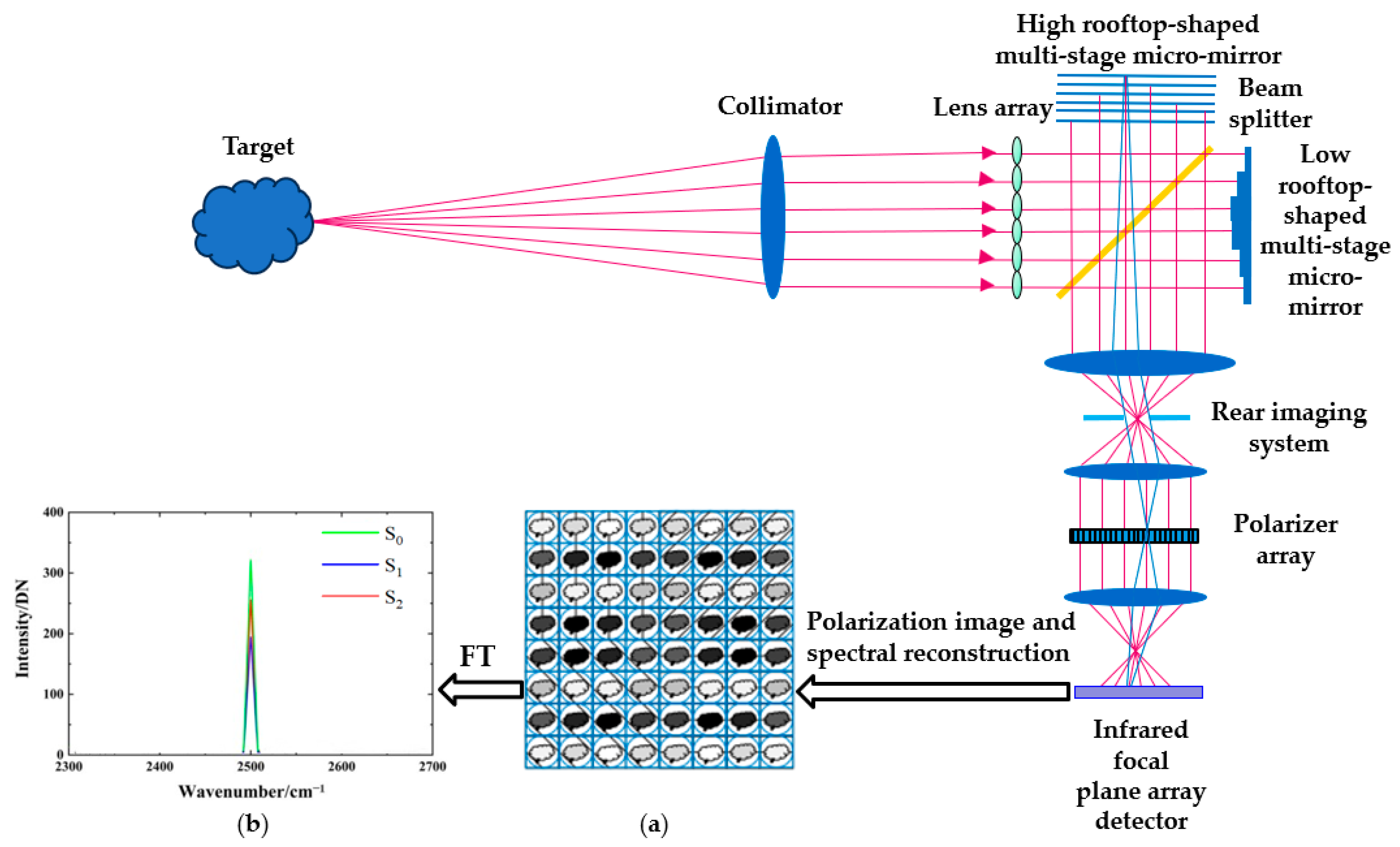
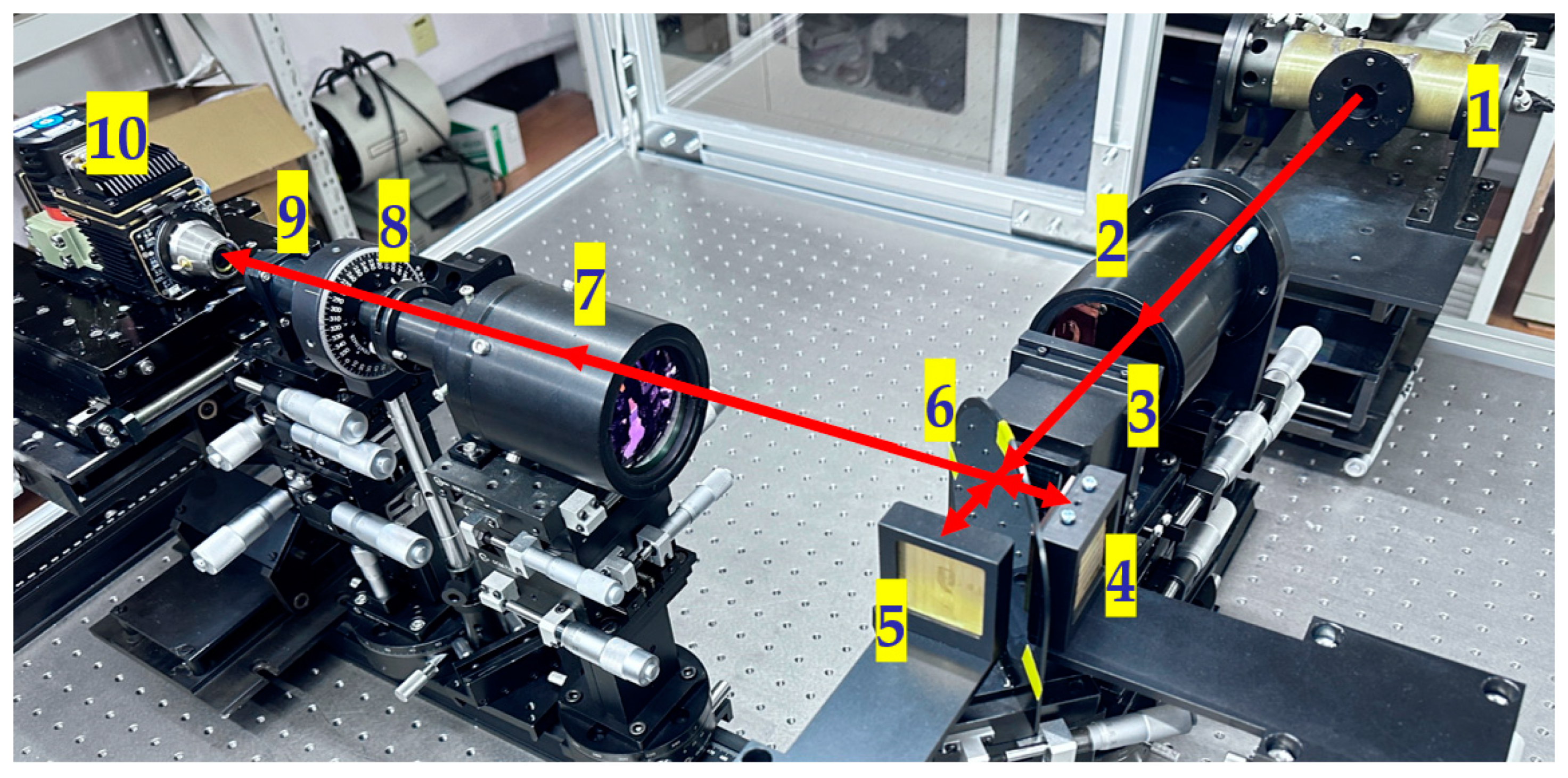
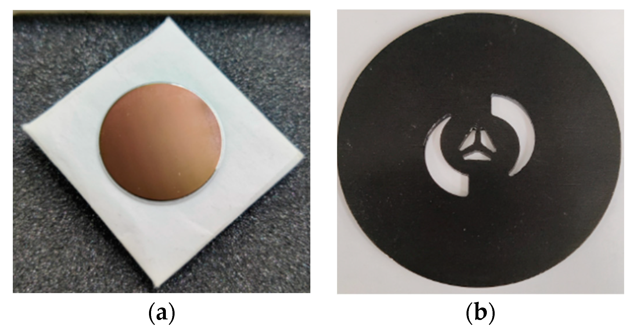
2.1. Principles of System Operation and Structural Parameters

The principle of a static infrared snapshot polarization spectroscopy imaging system is shown in Figure 1. The system consists of a pre-system, a micro-lens array, two multi-stage micro-reflectors, a beam splitter, a relay optical system, a polarizer array, and a detector. The target light field is incident into the multiplex imaging interferometer system through the collimation system, and the incident light field is imaged by the micro-lens array in multiple channels. Two high and low rooftop-shaped multi-stage micro-mirrors are placed orthogonally, and the step height conforms to the principle of optical path difference sampling complementarity. The imaging unit is subjected to distributed phase modulation to form an interference image array. The polarizer array modulates the interference image unit with different polarization states, so as to obtain the polarization-modulated interference image on the detector that is shown in Figure 1a as well as the polarization-modulated spectral image by Fourier transform, and to realize the polarization image reconstruction by Stokes polarization calculation that is shown in Figure 1b.

The system mainly works in the mid-infrared band; the spectral range is 3.7–4.8 μm, divided into 4 polarization interference channels; each polarization state corresponding to the number of interference channels is 8 × 8, the spectral resolution is 7.8 cm⁻¹, and the modulation transfer function of each optical element is greater than 0.5@17 lp/mm.

The core interferometric system of this system is composed of two orthogonal high- and low-stepped rooftop-shaped multi-stage micro-reflectors and a beam splitter, which contribute to the phase modulation of the imaging light field of the micro-lens array. The parameters of the rooftop-shaped multi-stage micro-reflector are as follows.

It can be seen from

Table 1. Design parameters of rooftop-shaped multi-stage micro-reflector.

Design Parameters	Value
Wavelength	3.7–4.8 μm
Left/right steps	8
Low-step height	10 μm
High-step height	80 μm
Width of steps	4 mm
Total length of reflector	64 mm

that the rooftop-shaped multi-stage micro-mirror has a total of 2 N = 16 steps, 8 on the left and 8 on the right, which satisfies the narrow-band sampling theorem. The sampling frequency F_s of the interferometer system is greater than 2 times the bandwidth BW of the emission spectral line of the detected target, and the height of the steps d meets the requirement of being less than or equal to 1/(4 BW). According to the spectral resolution Δ_ν = 1/(2 N²d) = 7.8 cm⁻¹, required by the system design, the low height of the steps d′ can be calculated to be 10 μm, with the high height of the steps Nd’ being 80 μm. The width of the steps matches the size of a single square lens of the micro-lens array (4 mm × 4 mm), and the total length of the mirror matches the number of lenses of the micro-lens array (16 × 16), which is made of silicon material, while the polarizer array is designed with a silicon substrate grid polarizer, so as to meet the working band of the system, which should be 3.7–4.8 μm. The system adopts the model Gavin615A HgCdTe material medium wave-refrigerated infrared detector, with a working wavelength of 3.7–4.8 μm, a pixel number of 640 × 512, a pixel size of 15 μm × 15 μm, an array size of 9.6 mm × 7.68 mm, an F# of 4, a cold shutter aperture of 5.1 mm, and a rear focal length of 19.8 mm. The system structure built is shown in Figure 2.

2.2. Principle of Polarization Pattern Decoupling and Information Reconstruction in PSIFTIS

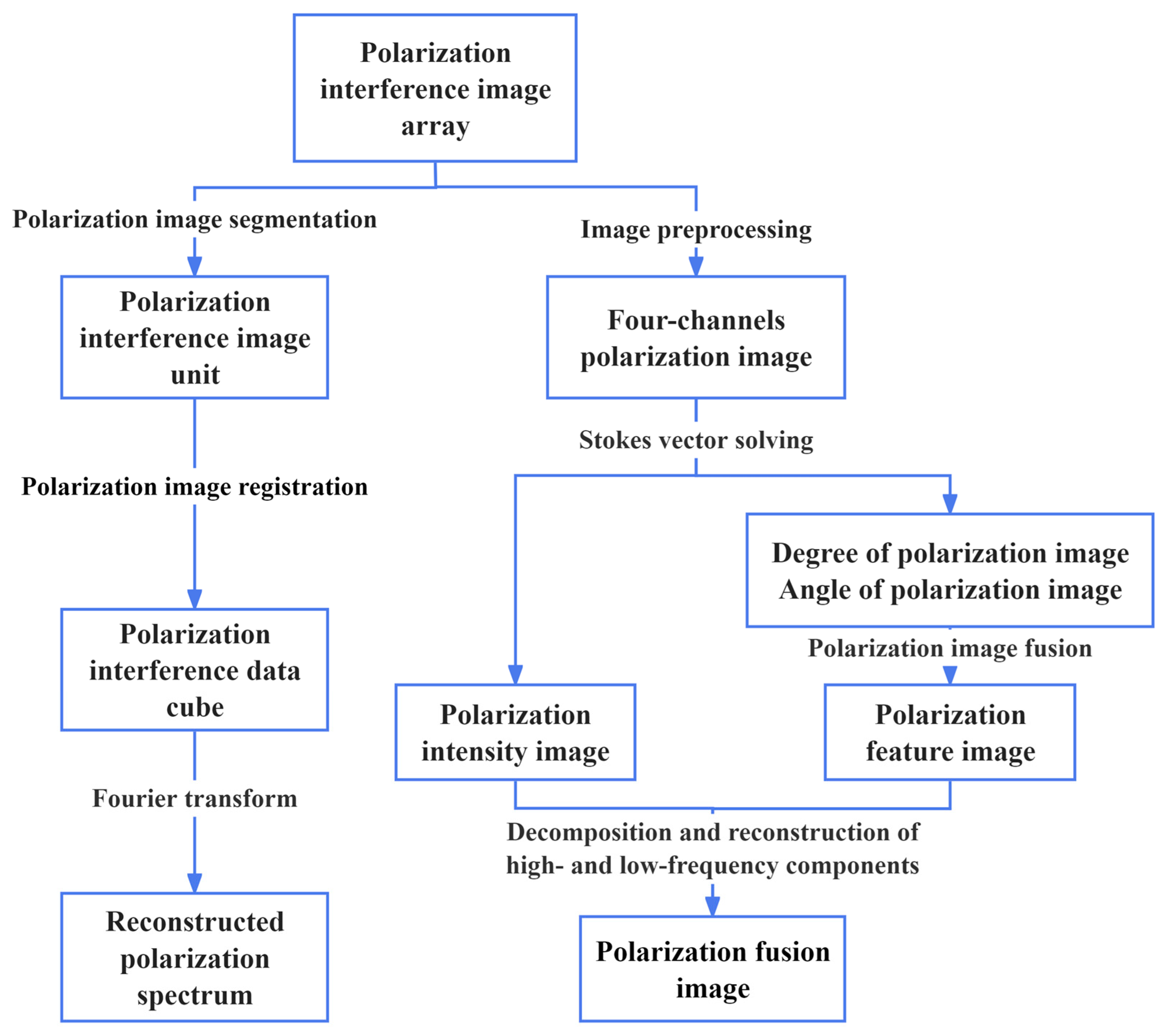
Because the data structure obtained by this system is relatively complex and the spatial, spectral, and polarization information are coupled together, in order to obtain the three-dimensional information of the target respectively, it is necessary to decouple and reconstruct the map of the polarization interference image array. The process of obtaining the reconstructed polarization spectrum and the polarization fusion image through the processing of the polarization interference image array data is shown in Figure 3.

The process is divided into two processing routes: the first route includes image segmentation, optical path difference matching, and image registration of a polarization interference image array to obtain the polarization interference intensity cube datasets I₀[x,y,Δ(m,n)], I₄₅[x,y,Δ(m,n)], I₉₀[x,y,Δ(m,n)], and I₁₃₅[x,y,Δ(m,n)], in polarization directions of 0°, 45°, 90°, and 135°, where (x,y) represents the spatial coordinate axis, Δ represents the optical path difference axis, m and n are the step orders of the high- and low-step micro-mirrors, (m,n) is the position coordinates of the corresponding phase modulation unit, and Δ(m,n) represents the modulated optical path difference generated by the phase modulation unit [18,19]. The interference intensity corresponding to the polarization direction is:

$$I_{\theta }\left[x,y,\Delta (m,n)\right]={\displaystyle {\int }_{{\nu }_{\min }}^{{\nu }_{\max }}{B}_{\theta }(x,y,\nu )}\exp [j2\pi \nu \Delta (m,n)]d\nu$$

(1)

Here, ν is the wave number, ν_min and ν_max represent the minimum and maximum wave number respectively, B_θ(x,y,ν) is the spectrum of each polarization direction, and the expression of the optical path difference is:

$$\Delta (m,n)=2(Qn-m)d$$

(2)

Here, Q is the series of rooftop-shaped stepped micro-mirrors, and d is the height of the lower step of the rooftop-shaped stepped micro-mirrors. With the array center as the zero point, the optical path difference increases in the horizontal and vertical directions. After addressing baseline correction and apodization, the polarization interference intensity data cube set I_θ[x,y,Δ(m,n)] is subjected to two-dimensional discrete Fourier transform to obtain the three-dimensional spectral data cube set B_θ(x,y,ν) of the target in each polarization direction, and the result is as follows:

$$B_{\theta }(x,y,\nu )=2d{\displaystyle \sum _m{\displaystyle \sum _n{I}_{\theta }(x,y,\Delta (m,n))\exp [-i4\pi \nu (Qn-m)d]}}$$

(3)

Each interferogram unit corresponds to a specific interference order under a specific polarization state, and polarization channel and interference channel are matched. According to the Stokes vector expression, the spectral information corresponding to each of the Stokes vectors S₀, S₁, S₂, and S₃ can be obtained as shown in Equation (4). S₀ represents the total intensity of light, S₁ represents the difference between 0° and 90° linearly polarized light components, S₂ represents the difference between 45° and 135° linearly polarized light components, and S₃ represents the difference between right-handed and left-handed circularly polarized light components. Since the amount of S₃ component in the reflected light of most objects in nature is very small, it is taken as approximately zero. The corresponding spectra of each Stokes component are:

$$\left\{\begin{array}{c}{B}_{S_0}(\nu )=B_{I_0}(\nu )+B_{I_{90}}(\nu )\\ B_{S_1}(\nu )=B_{I_0}(\nu )-B_{I_{90}}(\nu )\\ B_{S_2}(\nu )=B_{I_{45}}(\nu )-B_{I_{135}}(\nu )\end{array}\right.$$

(4)

The second route preprocesses the polarization interference image array to obtain four-channel infrared polarization images, and the Stokes parametric method is used to quantitatively describe the polarization state of the object. According to Equations (5) and (6), the degree of polarization (DoP) and angle of polarization (AoP) images can be calculated [20]:

$$DoP=\frac{\sqrt{{S_1}^2+{S_2}^2}}{S_0}$$

(5)

$$AoP=\frac{1}{2}\arctan (\frac{S_2}{S_1})$$

(6)

After obtaining the polarization intensity image, polarization degree image, and polarization angle image, the polarization degree image and polarization angle image are fused to obtain the polarization feature image, and then the polarization intensity image and the polarization feature image are decomposed into high- and low-frequency components by wavelet transform to obtain the polarization fusion image.

3. Algorithm Flow

3.1. Polarization Image and Spectral Decoupling and Spectral Reconstruction

The decoupling process of the polarization atlas is shown in Figure 4. According to the grayscale difference between image units of different interference order, the polarization interference image array is segmented by using the method of convolution kernel traversing the image and Canny edge detection. The interference order is determined by the phase space modulation mode of the system interference core device. The segmented image units are matched according to the optical path difference. The image units after the optical path difference matching are image-registered by SUSAN Corner Detection combined with the SIFT Feature Matching Algorithm, and the polarization interference intensity sequence of any point in the target scene is obtained. The polarization interference intensity of each polarization channel is transformed by Fourier transform to obtain the spectral information and polarization information of the target scene, and then the distributions of Stokes vectors of each polarization channel in the wavenumber domain, $B_{S_0}\left(v\right)$, $B_{S_1}\left(v\right)$, and $B_{S_2}\left(v\right)$, are obtained.

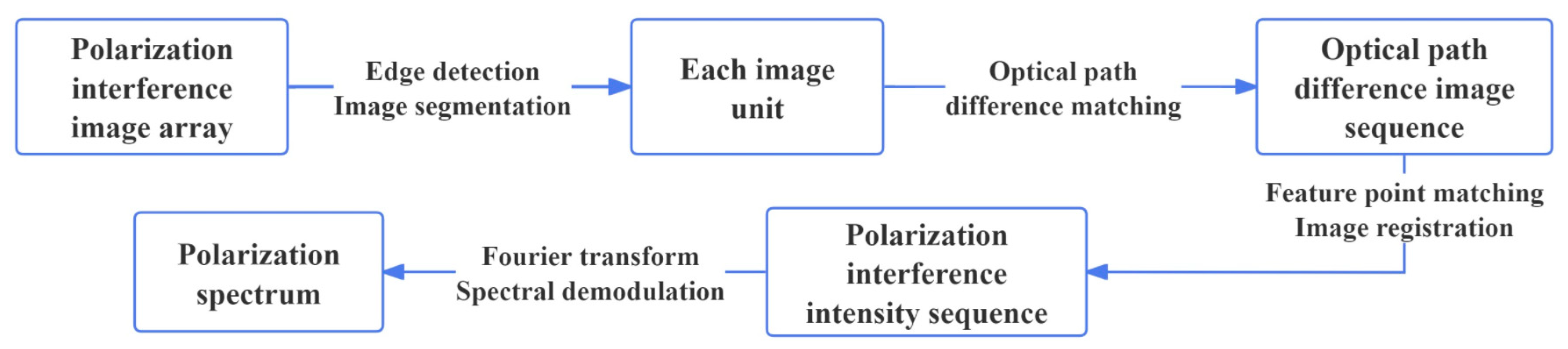
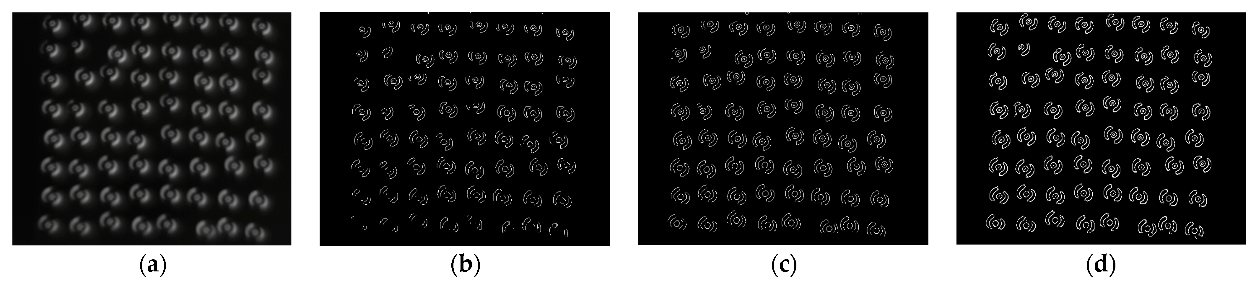
3.1.1. Polarization Interference Image Segmentation

The segmentation of the polarization interference image array is the basis of subsequent data processing. It can be seen from the system principle that the image array obtained by a single polarization channel of the detector should be arranged in a pattern of 8 × 8 with 64 image units of the same size. However, the manufacturing accuracy error and assembly error of the multi-stage micro-mirror, the manufacturing accuracy error of the micro-lens array, and the rotation translation error will lead to the alignment error of the optical system, which may cause different widths and order offsets of each interferogram unit, so it is necessary to segment the image units. Therefore, a method of convolution kernel traversal combined with the Canny Edge Detection Algorithm is proposed to realize image segmentation.

The method of using a single convolution kernel to traverse the image to obtain the rough location set of image elements is relatively effective, but there is also the problem of incomplete detected edges, while the Canny Edge Detection Algorithm has high accuracy in edge pixel location and can effectively suppress noise interference so that more fine edge information can be obtained; therefore, the combination of the two algorithms can improve the accuracy of edge detection so as to achieve more accurate image segmentation. The specific steps are as follows.

(1)

Adopt the convolution kernel with the size of the enclosing circle of a single image unit, and set a threshold to traverse the image to obtain the coarse positioning set of the image unit;

(2)

Carry out Canny edge detection on the image to obtain the image edge information positioning set;

(3)

Merge the ergodic coarse positioning set through the convolution kernel and the positioning set through Canny edge detection to obtain the accurate edge information set.

The coarse positioning point set W = ${\left\{Z_{\alpha }\right\}}_{\alpha =1}^{m_1}$ is obtained through the image processing of convolution kernel traversal, where m₁ represents the number of feature points. The measured image information positioning set V = ${\left\{Z_{\beta }\right\}}_{\beta =1}^{m_2}$ is obtained through Canny edge detection, where m₂ represents the number of feature points. The union set of the two is obtained as Y, which is the final precise edge information set, as shown in Equation (7):

$$Y=W\cup V={\left\{Z_{\alpha }\right\}}_{\alpha =1}^{m_1}\cup {\left\{Z_{\beta }\right\}}_{\beta =1}^{m_2}$$

(7)

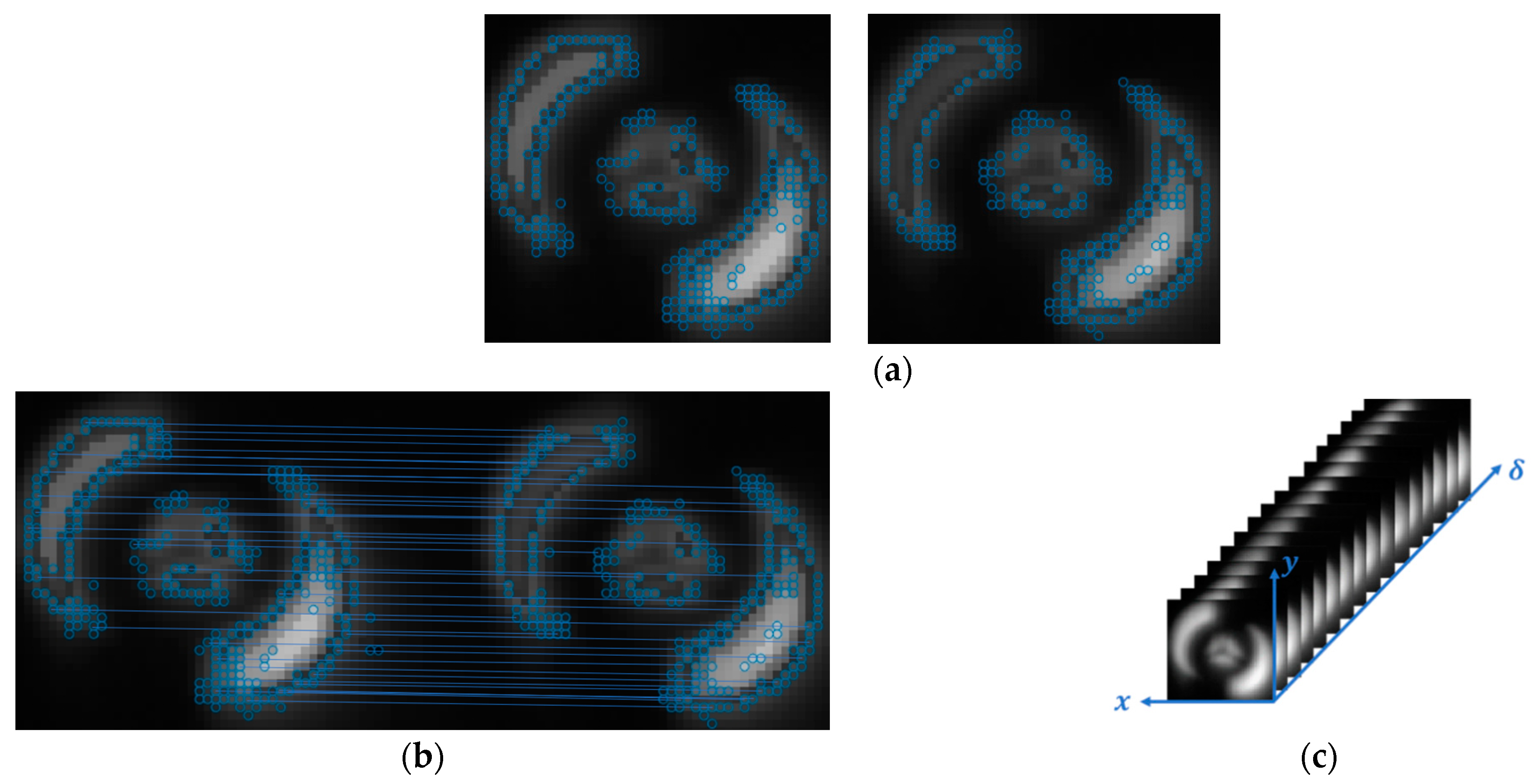
3.1.2. Polarization Interference Image Registration and Polarization Spectral Reconstruction

For the segmented image units, the interference order is determined by the phase space modulation mode of the system interference core device, and the segmented image units are matched according to the optical path difference. However, the polarization interference data cube set obtained by the optical path difference matching cannot accurately locate the image units, and there are large matching errors, which will affect the accuracy of spectral reconstruction. In order to accurately obtain the polarization interference intensity sequence of any point in the target scene to achieve high-precision spectral reconstruction, it is necessary to register the image units after the optical path difference matching. Therefore, this paper proposes an image registration algorithm based on SUSAN corner detection combined with SIFT feature matching.

The SIFT algorithm is a feature-matching algorithm based on scale space and using neighborhood gradient information to extract and describe features. SIFT features have good robustness to image rotation, scaling, and noise, but the feature point extraction is unstable, and most of the feature points are not corner points, which cannot well reflect the structural characteristics of the image. SUSAN corner detection is a feature point acquisition method based on grayscale level. It can detect the edge and corner of the image, and has the advantages of strong anti-noise ability, high precision, simpleness, and effectiveness. SUSAN corner detection is used to obtain the corner information of the image unit, and the SIFT descriptor is used to describe the feature point in the feature point description stage, so as to obtain stable and accurate feature point information. The specific steps are as follows.

(1)

Perform SUSAN corner detection for each image unit to obtain its corner information set

(2)

Generate SIFT feature descriptors according to the corner information set obtained in step (1);

(3)

Perform SIFT feature coarse matching and RANSAC feature fine matching for each image unit to obtain the feature point information set;

(4)

Take the intersection of the feature points obtained in step (1) and step (3) to obtain the final feature point set and complete image registration.

SUSAN corner detection is essentially a detection method based on a window template [21]. It uses a circular window of fixed size, directly compares the grayscale difference between the pixels in the circular window and the central pixel, counts the grayscale difference in the whole circular window, and uses the threshold judgment to detect corners. Since the process of SUSAN corner detection involves no image pixel gradient, it has good robustness in the presence of noise. Compared with the detection method based on gradient, situations where the central neighborhood and the central area angular response are difficult to distinguish are prevented, therefore a simple selection of local maximum values could lead to the non-maximum suppression.

After SUSAN corner detection, a preliminary corner information set is obtained, and then the SIFT feature matching algorithm is used to complete the corner information set and image registration [22]. The gradient magnitude and gradient amplitude of image pixels are obtained in the region with a radius of 3 × 1.5 σ (σ as the scale) based on the feature points through SUSAN Corner Detection, and then the gradient histogram is constructed, and the peak direction of the histogram becomes the main direction of the feature points. The region around the corner is rotated clockwise to the main direction angle, and a rectangular window of 16 × 16 with the corner as the center is selected in the rotated region, and then it is divided into 4 × 4 sub-regions. The gradient histogram of 16 sub-regions is constructed in 8 directions, and the 128-dimensional SIFT descriptor can be obtained. Then, the SIFT feature matching is completed. Finally, the outlier points are removed using the Random Sample Consensus (RANSAC) algorithm, to complete the image fine matching.

In order to make sure the obtained feature points are more accurate and more representative and the best are selected, the intersection of the feature point sets obtained through SUSAN corner detection and SIFT feature matching are taken as the final feature point set.

Then, image registration is carried out according to the position of feature points in image units to obtain the cube set of polarization interference intensity data, I_θ[x,y,Δ(m,n)], and then the polarization interference intensity sequence of feature points is obtained. After addressing baseline correcting and apodization by using the Gaussian function, a discrete Fourier transform is carried out to obtain the polarization spectrum cube B_θ(x,y,ν). The reconstructed polarization spectrum can be obtained by Equation (4).

3.2. Infrared Polarization Image Fusion

The spectral and polarization information of the target can be demodulated through a polarization interference image array. However, infrared images have inherent disadvantages such as large noise and low resolution, so the imaging quality of infrared images is also an important indicator of the system. Polarization image fusion can make full use of polarization information, make up for the disadvantage that a single intensity image cannot provide sufficient information under certain scene conditions, and further improve the amount of information obtained by optical detection. Therefore, the research on infrared polarization image fusion is carried out. Figure 5 is the overall flow chart of polarization image fusion.

3.2.1. DoP and AoP Image Solution and Polarization Feature Image Fusion

In order to reduce the impact of pixel position difference and noise pollution, it is necessary to denoise and register the image in advance. In this paper, a grayscale transformation is adopted to enhance the image contrast, and the polarization images of 0°, 45°, 90°, and 135° after pretreatment are calculated to obtain S₀, S₁, and S₂ images. Then, the polarization degree and polarization angle images are calculated according to Equations (5) and (6). DoP and AoP images can provide a lot of target details in the fusion process, which plays an important role in improving image quality. DoP images can highlight the polarization characteristic information of the target; AoP images have a low signal-to-noise ratio but contain many detailed texture information. The two images can be fused to remove redundancy and increase useful information of the image, and play a role in the subsequent fusion with the intensity image. In order to make better use of the complementarity between images, this paper chooses the minimum value fusion method, which can be described as follows:

$$C_F(\eta ,\xi )=\left\{\begin{array}{c}{C}_A(\eta ,\xi ),\hspace{1em}\left|C_A(\eta ,\xi )\right|\le \left|C_B(\eta ,\xi )\right|\\ C_B(\eta ,\xi ),\hspace{1em}\left|C_A(\eta ,\xi )\right|>\left|C_B(\eta ,\xi )\right|\end{array}\right.$$

(8)

Here C_A(η,ξ) and C_B(η,ξ) are a set of decomposition coefficients of source image A and source image B respectively, and C_F(η,ξ) is the coefficient after fusion.

3.2.2. High- and Low-Frequency Components’ Decomposition of PI and PF Images

The PI and PF images acquired are then decomposed into high- and low-frequency components using the Haar wavelet transform. As the Haar wavelet transform is an orthogonal wavelet with both symmetry and finite support, it serves as the only orthogonal wavelet that possesses these characteristics. These images come with a typical two-dimensional discrete signal, thus we extend the one-dimensional discrete wavelet transform to a two-dimensional function in order to achieve the two-dimensional discrete wavelet transform of the image. In two-dimensional contexts, each two-dimensional wavelet can be expressed as the product of two one-dimensional wavelets, resulting in 4 separable scale functions, which enable the measurement of grayscale variations within the image along different directions. φ(x,y) is the low-frequency scale change, Ψ^H(x,y) is the high-frequency horizontal edge change, Ψ^V(x,y) is the high-frequency vertical edge change, and Ψ^D(x,y) is the high-frequency diagonal change.

3.2.3. High- and Low-Frequency Components’ Fusion of the Polarization Image

Fusion rules are crucial for image fusion, with the selection principle being to retain useful information while avoiding useless information and enhancing the fusion effect through complementarity and redundancy between images. After obtaining the high- and low-frequency components of the polarization intensity image and the polarization feature image, different fusion rules are used to fuse the high- and low-frequency components of the two images.

(1)

Low-Frequency Fusion of a Polarized Image

The low-frequency part of the image represents the main information component of the image, represents the main energy distribution in the image, and reflects the main features of the image. In this paper, the low-frequency fusion rule of the region coefficient difference combined with the average gradient grayscale stretch (RCD-AG-GS) is adopted. While preserving the image information to the maximum extent possible, the clarity of the image is further enhanced.

Firstly, the low-frequency components of the two images are grayscale stretched to enhance the contrast of the image. Then, the low-frequency fusion coefficients are preliminarily confirmed by using the difference of regional coefficients. The difference of regional coefficients is the difference between the grayscale value of the pixel and the average energy of the region in which it is located. The greater the difference is, the more useful information the pixel has. Its expression is [23]:

$${‖e_i(x,y)‖}_{M\times N}={\displaystyle \sum _{m″=(1-M)/2}^{(M-1)/2}{\displaystyle \sum _{n″=(1-N)/2}^{(N-1)/2}\left|\left|f_i(x+m″,y+n″)\right|-\overline{e}{(x,y)}_{M\times N}\right|}}$$

(9)

$$\overline{e}{(x,y)}_{M\times N}=\frac{{\displaystyle \sum _{m″=-(M-1)/2}^{(M-1)/2}{\displaystyle \sum _{n″=-(N-1)/2}^{(N-1)/2}\left|f_i(x+m″,y+n″)\right|}}}{M\times N}$$

(10)

Here, i represents the PI and PF images, e represents the low-frequency component, f represents the grayscale value of a pixel, and ē(x,y)_{M × N} represents the mean of the absolute grayscale value of the low-frequency part in an M × N slider area.

However, if the region coefficient difference is only used for fusion, useless information will also be fused into the image, resulting in a lower fusion effect and blurring. Therefore, the clarity needs to be improved. The average gradient can well reflect the tiny details and texture characteristics of the image, as well as the clarity of the image. Therefore, it is combined with the region coefficient difference to achieve effective fusion of the low-frequency components. The expression of the average gradient is as follows:

$$\nabla {\overline{g}}_i=\frac{1}{(M-1)\times (N-1)}{\displaystyle \sum _{i=1}^{M-1}{\displaystyle \sum _{j=1}^{N-1}\sqrt{\frac{{[f(i,j)-f(i+1,j)]}^2+{[f(i,j)-f(i,j+1)]}^2}{2}}}}$$

(11)

Here, f(i,j) is the grayscale value of the i-th row and j-th column of the image; M and N are the total number of rows and columns of the image, respectively. When the difference of the regional coefficients of the low-frequency components of two images is not equal, the grayscale value of the one with a larger difference is taken to determine the low-frequency fusion coefficient. Meanwhile, when the difference of the regional coefficients of the low-frequency components of two images is equal, the grayscale value of the one with a larger average gradient is taken as the low-frequency fusion coefficient. By combining Equations (9)–(11), the specific selection rule of the low-frequency fusion coefficient of the fused image can be obtained, as shown in Equation (12):

$$f_i(x,y)=\left\{\begin{array}{c}{f}_{PI}(x,y),\hspace{1em}{‖e_{PI}(x,y)‖}_{M\times N}>{‖e_{PF}(x,y)‖}_{M\times N}\\ f_{PF}(x,y),\hspace{1em}{‖e_{PI}(x,y)‖}_{M\times N}<{‖e_{PF}(x,y)‖}_{M\times N}\\ f_{PI}(x,y),\hspace{1em}{‖e_{PI}(x,y)‖}_{M\times N}={‖e_{PF}(x,y)‖}_{M\times N},{‖\nabla {\overline{g}}_{PI}‖}_{M\times N}\ge {‖\nabla {\overline{g}}_{PF}‖}_{M\times N}\\ f_{PF}(x,y),\hspace{1em}{‖e_{PI}(x,y)‖}_{M\times N}={‖e_{PF}(x,y)‖}_{M\times N},{‖\nabla {\overline{g}}_{PI}‖}_{M\times N}<{‖\nabla {\overline{g}}_{PF}‖}_{M\times N}\end{array}\right.$$

(12)

(2)

High-Frequency Fusion of a Polarized Image

The high-frequency component of an image generally reflects the part of the image with a sharp grayscale transformation, contains a large number of image details and characteristic information, and can distinguish the object and scene in the image well. The high-frequency part after wavelet decomposition is divided into vertical, horizontal, and diagonal components. In this paper, the fusion rules of taking the maximum energy of the weighted region are used to fuse the three components. This method can effectively highlight the image texture and detailed information.

The energy algorithm of an image calculates the grayscale value of an image or a certain region, while the energy of a region is found from calculating the grayscale value of a single pixel and its neighborhood within the range. The square neighborhood (x − k, y − k, x + k, y + k) of a pixel (x,y) is defined as the region Ω, then the energy of the region can be expressed as:

$$E(x,y)={\displaystyle \sum _m{\displaystyle \sum _n\mathrm{\Omega }(h,l)}}{f}^2(h,l)$$

(13)

Here, (h,l)∈Ω, Ω(h,l) is the weighted value, taking the pixel point (x,y) as the center, and the weight gradually decreases away from the center. f(h,l) is the grayscale value at (h,l). The regional energy matching degree is defined as:

$$M_{PIF}(x,y)=\frac{2{\displaystyle \sum _m{\displaystyle \sum _n\mathrm{\Omega }(h,l)f_{PI}(h,l)f_{PF}(h,l)}}}{E_{PI}(x,y)+E_{PF}(x,y)}$$

(14)

Here, the value range of M_PIF(x,y) is [0,1], and the higher the value is, the higher the regional energy matching degree is and the smaller the energy difference is. The matching degree threshold is set as δ. When M_PIF(x,y) < δ, the grayscale value of the high-frequency component of the polarization intensity image and polarization characteristic image with larger regional energy is taken as the high-frequency fusion coefficient. When M_PIF(x,y) ≥ δ, the weighted fusion is carried out according to the size of the regional energy and the size of the regional energy matching degree, and the obtained value is taken as the high-frequency fusion coefficient. In summary, by combining Equations (13) and (14), the specific selection rule of the high-frequency fusion coefficient of the fused image can be obtained as shown in Equation (15):

$$F_i(x,y)=\left\{\begin{array}{cc}{f}_{PI}(x,y),& M_{PIF}(x,y)<\delta ,E_{PI}(x,y)\ge E_{PF}(x,y)\\ f_{PF}(x,y),& M_{PIF}(x,y)<\delta ,E_{PI}(x,y)<E_{PF}(x,y)\\ (1-M_{PIF}(x,y))f_{PI}(x,y)+M_{PIF}(x,y)f_{PF}(x,y),& M_{PIF}(x,y)\ge \delta ,E_{PI}(x,y)<E_{PF}(x,y)\\ M_{PIF}(x,y)f_{PI}(x,y)+(1-M_{PIF}(x,y))f_{PF}(x,y),& M_{PIF}(x,y)\ge \delta ,E_{PI}(x,y)\ge E_{PF}(x,y)\end{array}\right.$$

(15)

3.2.4. Image Reconstruction Using Inverse Haar Wavelet Transform

The inverse Haar wavelet transform is performed on the obtained low-frequency and high-frequency coefficients to complete the reconstruction of high- and low-frequency components. According to Equations (12) and (15), the fusion coefficients of each component are as follows:

$$\left\{\begin{array}{c}{\phi }^{\prime }(x,y)=f_i(x,y)\\ {\mathrm{\Psi }}^{H^{\prime }}(x,y)={F_i}^H(x,y)\\ {\mathrm{\Psi }}^{V^{\prime }}(x,y)={F_i}^V(x,y)\\ {\mathrm{\Psi }}^{D^{\prime }}(x,y)={F_i}^D(x,y)\end{array}\right.$$

(16)

4. PSIFTIS Imaging Experiment Results and Data Processing

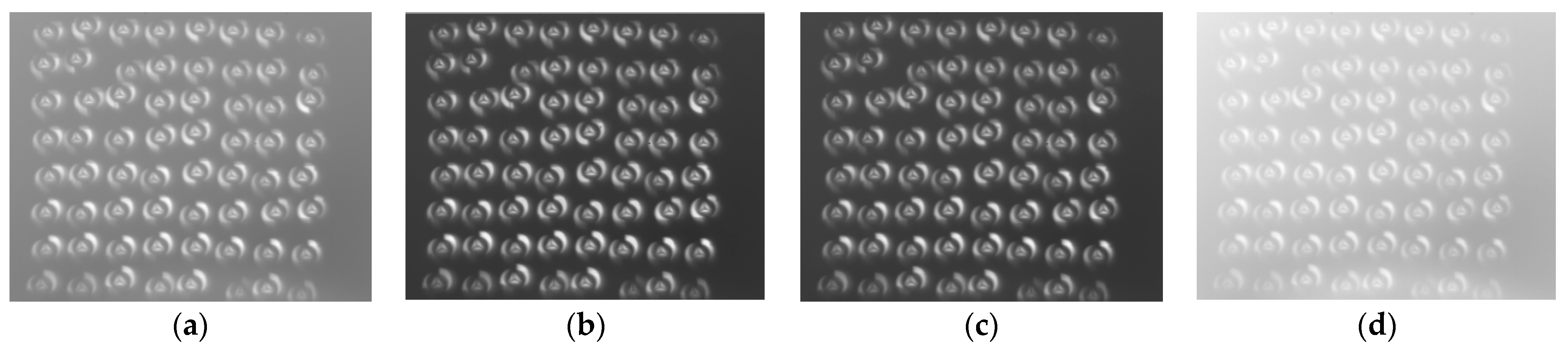
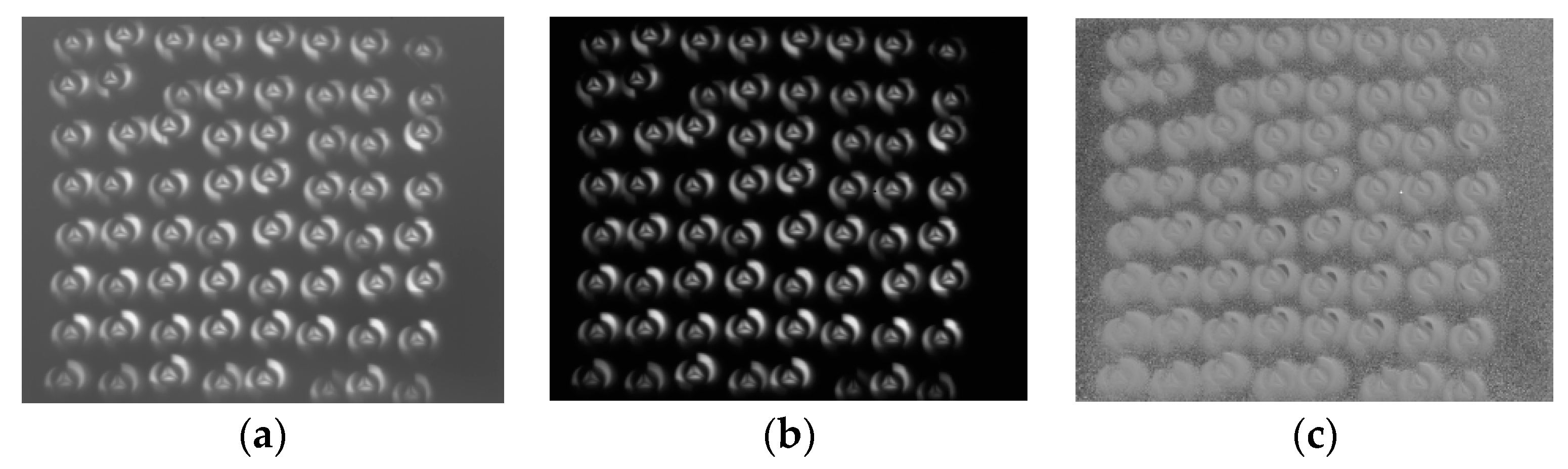
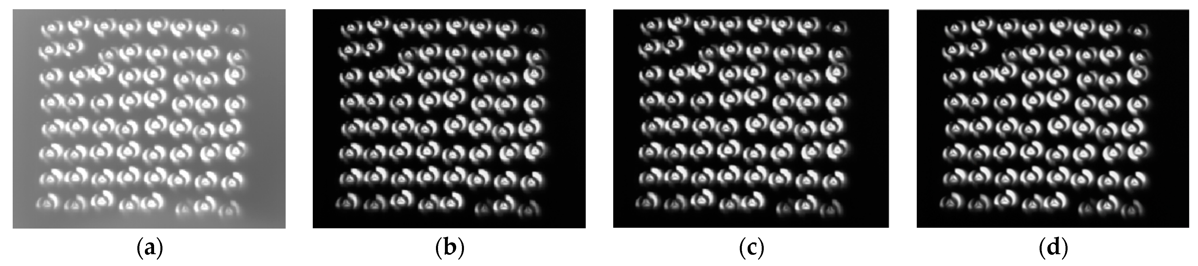
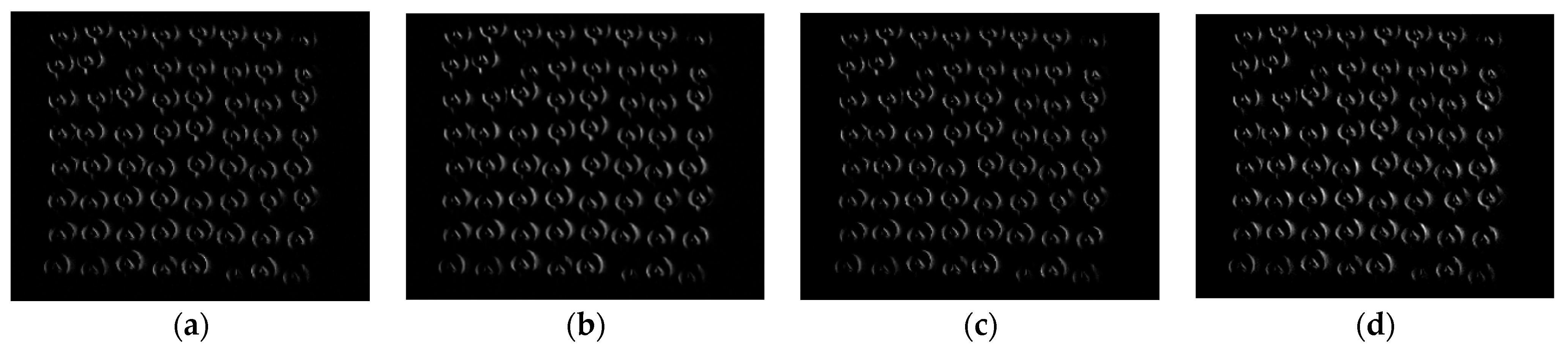
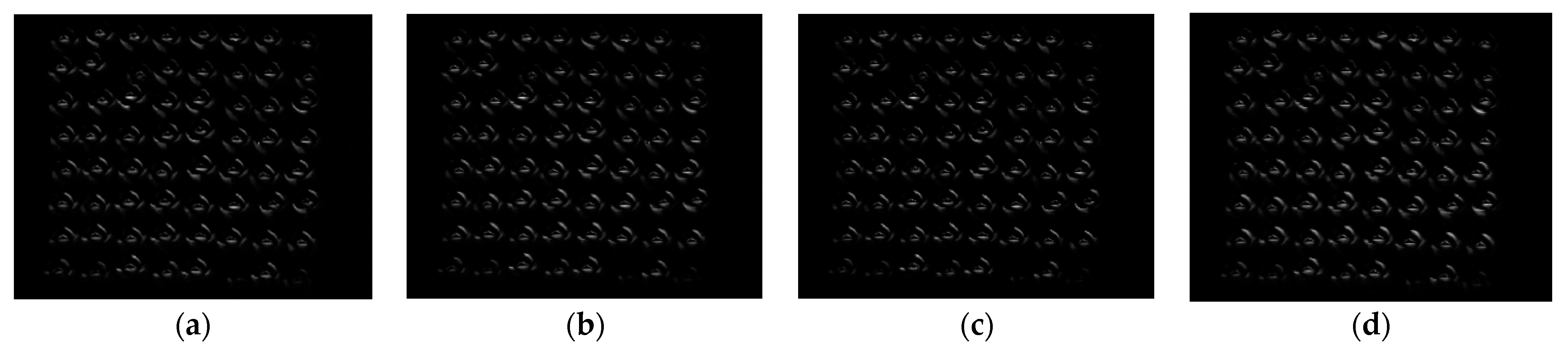
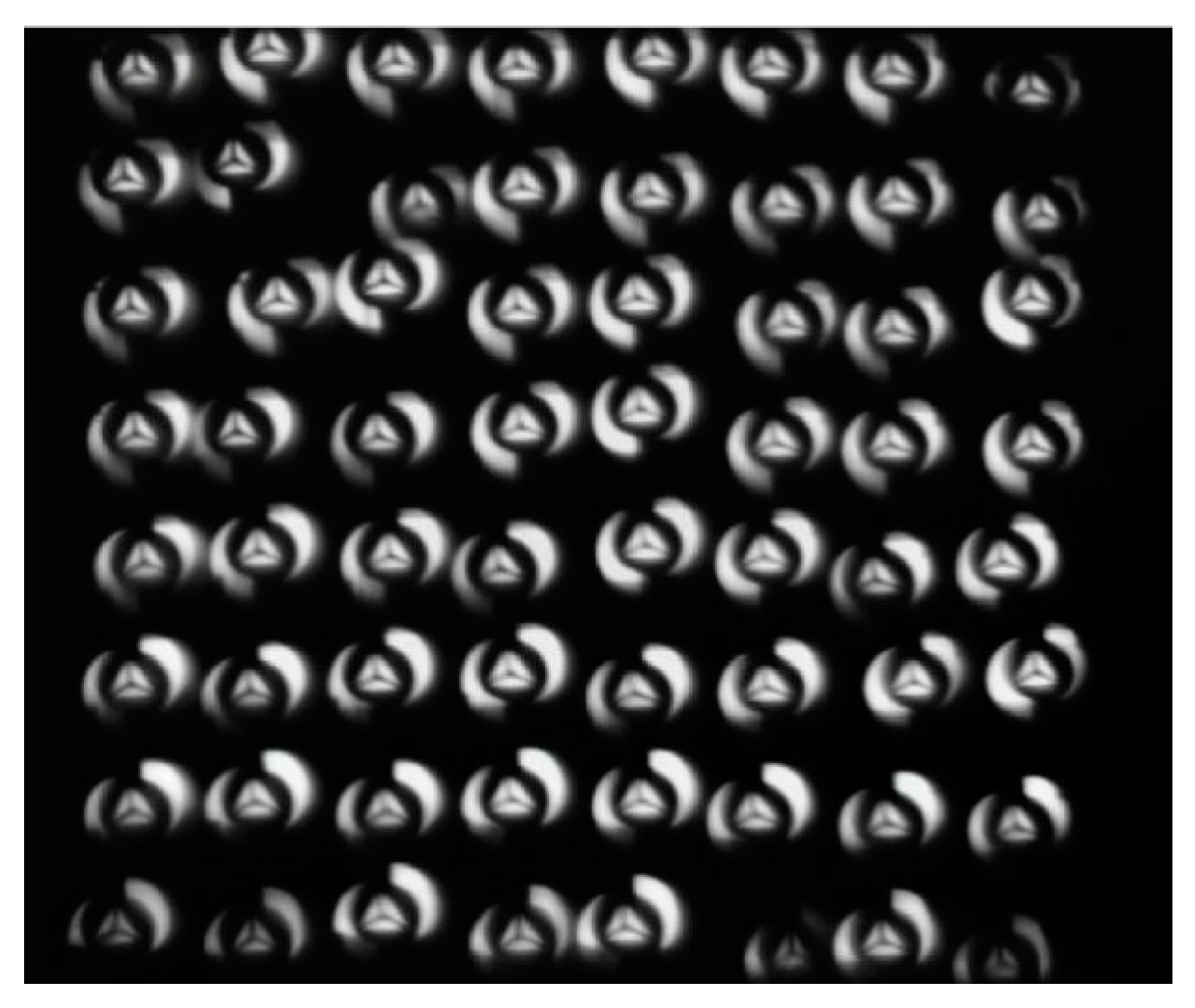
4.1. Polarization Interferometric Image Acquisition and Decoupling

To complete the processing of system spectrum information, an experimental platform was set up in the laboratory environment. Narrow-band filters with central wavelengths of 3800 nm, 3970 nm, and 4720 nm are adopted, whose specifications are Ø25.4 × 1 mm, Ø25.4 × 1 mm, and Ø25.4 × 0.5 mm, respectively. The half-peak widths are 76 ± 10 nm, 40 ± 10 nm, and 90 ± 10 nm. The images of the filters are shown in the Figure 6a. The target used in the experiment is shown in Figure 6b.

When the system performs imaging experiments on the target, polarization interference image arrays will be formed on the detector array. Taking 45° polarization as an example, as shown in Figure 7a, the polarization interference image arrays are segmented according to the above methods, and the results are shown in Figure 7d.

As can be seen from the results, the convolution kernel traversal image in Figure 7b makes a rough location of the edge, and the edge closure is not good. Figure 7c shows the location results of the Canny edge detection method, which indicates that the image edge contour location effect is good and the edge closure is good. Finally, the convolution kernel traversal rough location and Canny edge detection location results are merged to obtain the results shown in Figure 7d.

Then, the image units after optical path difference matching are registered in optical path order. As shown in Figure 8a, the results of two image units obtained by using the SUSAN corner detection method show that the number of the corner detection was moderate. The results after coarse SIFT feature matching and fine RANSAC feature matching are in Figure 8b, showing that the number of matching lines is moderate and the matching degree is good. After registration of all image units after feature matching, a polarization interference data cube set of each polarization channel is obtained as shown in Figure 8c.

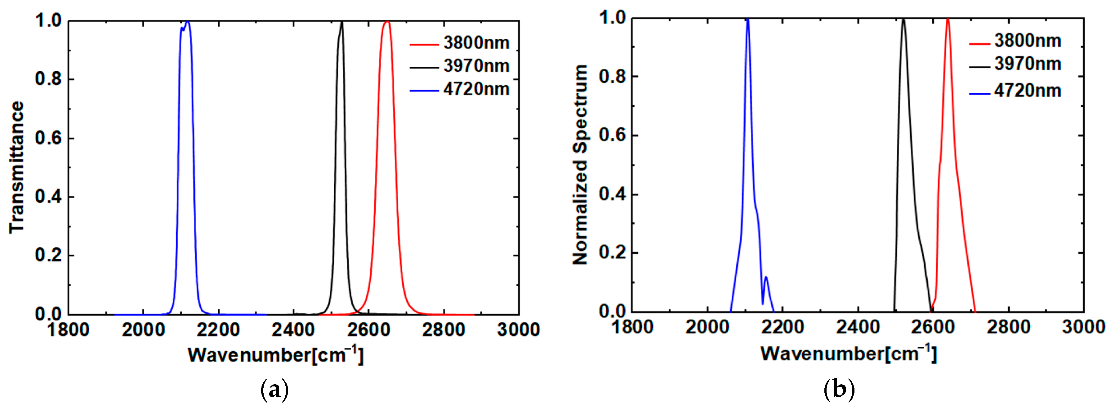
4.2. Polarization Spectral Reconstruction

In order to obtain the polarization spectrum and image information of the target, a carbon–silicon rod light source was used as the active light source. Narrow-band filters with central wavelengths of 3800 nm (2644.64 cm⁻¹), 3970 nm (2522.93 cm⁻¹), and 4720 nm (2111.72 cm⁻¹) were selected respectively, and the theoretical spectral information of the narrow-band filters was used to verify the spectral information of the target. The experimental results were displayed in the 0° polarization channel, and the wavenumber calibration methods of other polarization channels were the same. The theoretical spectra of each filter group in the 0° polarization channel are shown in Figure 9a.

In order to solve the problem of wavenumber drift of a spectral line caused by tilting and pitching errors generated during the processing and adjustment of a multi-stage micro-mirror, wavenumber calibration experiments were conducted. The filter plates of each central wavelength were assembled into the system, and the polarization interference image arrays after adding the filter plates of each central wavelength were measured respectively. The decoupling of the spectrum was completed according to the above method, and the reconstructed spectrum was obtained after discrete Fourier transform, as shown in Figure 9b. Since the tilt and slope errors of the rooftop-shaped multi-stage micro-mirror cause linear wavenumber drift to the spectrum, the linear error transfer model of the wavenumber drift is:

$$\nu \prime =k_1\nu +b_1$$

(17)

Here, ν′ is the spectral wave number after calibration, and ν is the spectral wave number actually measured. The gain coefficient k₁ is 0.9974 and the bias coefficient b₁ is 11.9597 obtained through linear fitting, so the linear fitting model is:

$$\nu \prime =0.9974\nu +11.9597$$

(18)

The calibrated central wavenumbers are 2642.98 cm⁻¹, 2525.05 cm⁻¹, and 2111.24 cm⁻¹, respectively, and the wavenumber errors are 1.66 cm⁻¹, 2.12 cm⁻¹, and 0.48 cm⁻¹, respectively. The wavenumber errors are all less than 1/2 of the theoretical spectral resolution (7.8 cm⁻¹), which proves that the calibrated central wavenumbers are basically in accordance with the theoretical wavenumbers.

After the accuracy of the spectral wavenumber measurement was verified by wavenumber calibration, spectral data detection was performed on the high-temperature target to obtain the target polarization spectral information. The target (as shown in Figure 6b) was subjected to target imaging experiments with 38° polarized light incident in the system with a 3970 nm central wavelength filter.

According to the spectral decoupling method mentioned above, the polarization interference intensity data cube of the target’s four polarization directions, I_θ[x,y,Δ(m,n)], can be obtained. The polarization interference intensity sequences corresponding to the characteristic pixel point (10.6) of the polarization interference image unit selected at the central wavelength of 3970 nm are shown in Figure 10.

The polarization interference intensity sequence is addressed, baseline-corrected, and apodized, and then subjected to two-dimensional discrete Fourier transform to obtain the spectral information B_θ(x,y,ν) of each polarization channel. The reconstruction spectra of each polarization channel and Stokes vector spectral lines can be obtained by Equation (4), as shown in Figure 11.

The reconstructed spectra show that in the system with a 3970 nm filter, the wavenumber errors of the maximum spectral peak corresponding to the four polarization channels are 1.82 cm⁻¹, 0.12 cm⁻¹, 1.67 cm⁻¹, and 0.03 cm⁻¹ respectively, and the reconstructed spectra are well consistent with the theoretical spectral lines. The maximum spectral peak corresponding to the four polarization channels are 37.377, 75.140, 56.767, and 23.388, respectively. The Stokes vector peaks are 94.145, 19.491, and 53.184, respectively. According to Equation (6), the polarization direction of incident light can be calculated as 38.704°, which differs from the actual incident polarization angle of 38° by 0.704°, with an error of less than 1°. In summary, the reconstructed polarization spectra have good accuracy.

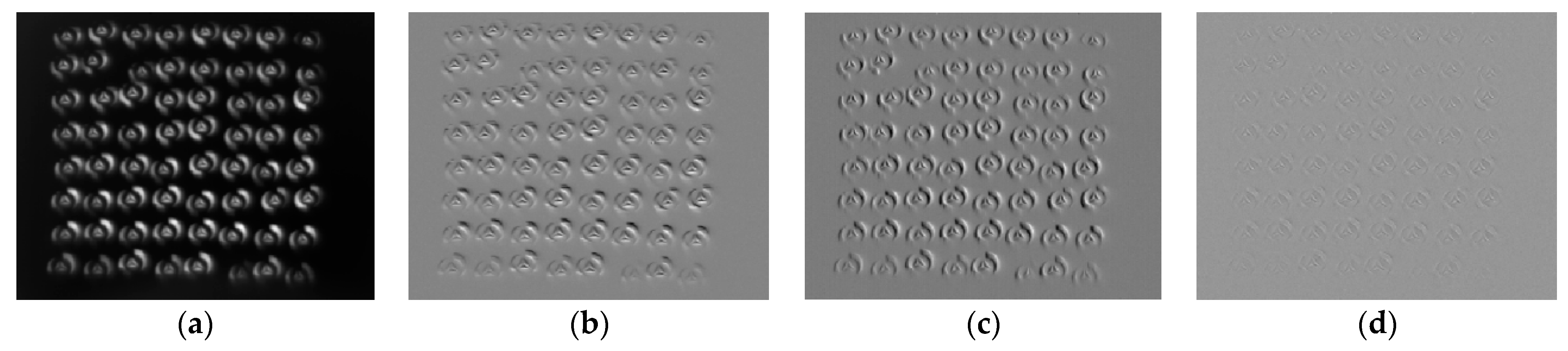
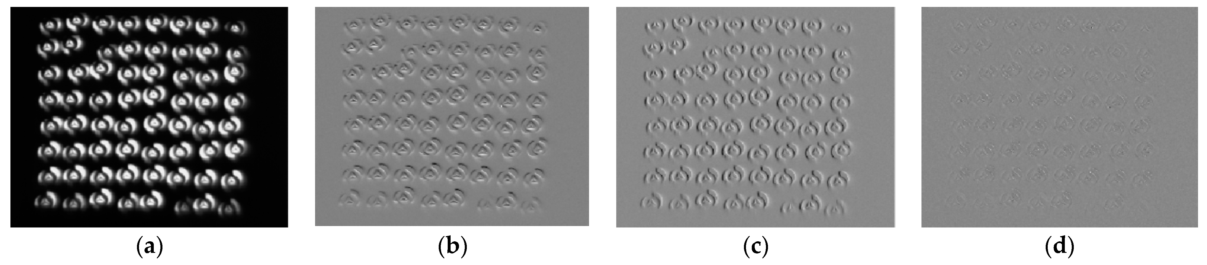
4.3. Infrared Polarization Image Fusion

A carbon–silicon rod light source is used as the active light source with a polarizer attached behind. It is verified that the system has polarization components in each polarization direction, which meets the universality of instruments. Therefore, this paper takes a light source that simulates a polarization angle of 38° as an example for the study on polarization image fusion. The displacement between image units would occur due to the machining error of the micro-lens array in the system, and the crosstalk between interference channels would also make the brightness of image units uneven, which would affect the final imaging quality of the system. Therefore, it is necessary to extract useful information or features of each image and fuse them to improve the quality and clarity of the image. The polarization images of 0°, 45°, 90°, and 135° obtained through experiments are preprocessed to obtain four infrared polarization images, as shown in Figure 12.

Next, the polarization solution is performed by using the existing polarization images, and the DoP and AoP images are obtained as shown in Figure 13.

Images of the PI, DoP, and AoP are obtained as shown in Figure 13a–c. Polarization image fusion is performed on DoP and AoP images by using the pixel-based image fusion mean value method, maximum value method, and minimum value method, and the results are shown in Figure 14.

It can be seen from subjective observation that the image of the minimum value fusion method is clearer and brighter, and the edge details are also enhanced, so this has the best imaging effect among the three methods. The objective index is evaluated by the PSNR (peak signal-to-noise ratio). The PSNR of the DoP image is 5.9090 dB, and the PSNR of the AoP image is 14.1327 dB. The PSNR of the mean value fusion image is 11.8186 dB, the PSNR of the maximum value fusion image is 8.0655 dB, and the PSNR of the minimum value fusion image is 14.7940 dB. It can be seen that the peak signal-to-noise ratio of the minimum value fusion image is higher than that of the other two fusion methods and higher than that of the AoP and DoP images.

The PI and PF images obtained previously were decomposed into one low-frequency component and three high-frequency components by using the Haar wavelet transform, as shown in Figure 15 and Figure 16.

In order to verify the effectiveness of the fusion algorithm of the low-frequency region coefficient difference combined with average gradient grayscale stretching (RCD-AG-GS) in Section 3.2.3.(1) above, the fusion rule of taking the maximum of the region contrast, the maximum of the region energy, and the minimum of the region energy is selected to compare with the algorithm in this paper, and the objective evaluation function indexes such as average gradient (AG), peak signal-to-noise ratio (PSNR), information entropy (EN), and mutual information (MI) are used to quantitatively evaluate the quality of the fused image. Different low-frequency component fusion rules are shown in Figure 17, and the pairs of objective evaluation indexes are shown in

Table 2. Evaluation and analysis of different low-frequency component fusion rules.

	AG	PSNR	EN	MI
PI	7.2223	4.5937	6.4100	/
PF	10.0424	10.5546	6.4107	/
Maximum Value of Regional Energy	8.2208	4.6046	6.4335	8.3545
Maximum Value of Regional Contrast	11.7738	10.5546	6.4766	8.3139
Minimum Value of Regional Energy	11.7746	10.3954	6.4806	8.3181
RCD-AG-GS	13.1196	57.5921	6.4772	12.9612

.

From the analysis of the objective evaluation function indexes of the fused image, the RCD-AG-GS fusion rules adopted in this paper have excellent performance in the root mean square error, peak signal-to-noise ratio, and mutual information indexes, which greatly outperform other fusion rules. In the information entropy index, they are basically equal to other methods and better than the initial two images.

In order to verify the effectiveness of the fusion algorithm for the maximum value of high-frequency weighted area energy in Section 3.2.3.(2) above, the fusion rules of taking the maximum value of regional contrast, the average value of the corresponding pixels, and the minimum value regional energy are selected to compare with the algorithm in this paper. The fusion effects of high-frequency vertical, horizontal, and diagonal components are shown in Figure 18, Figure 19 and Figure 20 and the objective index analysis data are shown in

Table 3. Evaluation of different high-frequency vertical component fusion rules.

	MSE	PSNR	EN	MI
PI	10.7134	37.8315	1.0850	/
PF	10.0424	37.8934	1.1052	/
Maximum Value of Regional Contrast	10.5619	37.8934	1.1422	1.7644
Average Value of Corresponding Pixels	9.5830	37.8552	1.2031	1.6510
Minimum Value of Regional Energy	13.8219	36.7251	1.0569	1.7961
Maximum Value of Weighted Regional Energy	7.5514	39.3505	1.2660	2.0668

,

Table 4. Evaluation of different high-frequency horizontal component fusion rules.

	MSE	PSNR	EN	MI
PI	9.2040	38.4910	1.0768	/
PF	10.4426	37.9427	1.0896	/
Maximum Value of Regional Contrast	10.4424	37.9428	1.1076	1.6908
Average Value of Corresponding Pixels	9.1250	38.5285	1.1094	1.5396
Minimum Value of Regional Energy	12.4729	37.1711	1.0720	1.6575
Maximum Value of Weighted Regional Energy	7.2628	39.5198	1.1336	2.0651

and

Table 5. Evaluation of different high-frequency diagonal component fusion rules.

	MSE	PSNR	EN	MI
PI	0.1326	56.9048	0.2772	/
PF	0.5865	50.4480	0.7176	/
Maximum Value of Regional Contrast	0.5864	50.4480	0.2704	0.3121
Average Value of Corresponding Pixels	0.2245	54.6178	0.2075	0.2150
Minimum Value of Regional Energy	0.6054	50.3105	0.2561	0.2570
Maximum Value of Weighted Regional Energy	0.1171	57.4456	0.7341	0.7277

.

From the above fusion images of high-frequency vertical, horizontal, and diagonal components and objective evaluation function indexes, it can be seen that the objective evaluation function indexes of the image with the fusion rule of taking the maximum value of the high-frequency weighted regional energy are better than the source image and other fusion rules. The root mean square error is significantly reduced, and the peak signal-to-noise ratio, information entropy, and mutual information indexes are all improved. Subjectively, the image processed by the fusion rule selected in this paper is relatively clearer, and the details are more specific.

Then, the inverse Haar wavelet transform is performed on the obtained low-frequency and high-frequency coefficients to complete the reconstruction of high- and low-frequency components, and the fused polarization image array is obtained as shown in Figure 21. The results after comparison with the average values of various indicators of the initial images with different polarization directions are shown in

Table 6. Evaluation and analysis of polarimetric image array fusion.

	0° Polarization	45° Polarization	90° Polarization	135° Polarization	Means of Different Polarization Images	Fusion Polarization Image Array
PSNR	34.7211	34.8012	34.7931	34.7033	34.7547	56.0787
AG	7.5988	8.9013	8.4875	6.0465	7.7585	11.4275
EN	6.6616	6.7024	6.7536	6.5899	6.6769	7.2470

. In terms of objective indicators, the peak signal-to-noise ratio of the fused image is increased by 61.4%, the average gradient is increased by 47.3%, and the information entropy is increased by 8.5%, which fully shows that the fused image has more information and shows more details.

Because each image unit in the polarization image array has a small number of pixels, the polarization image array obtained by fusion is reconstructed with pseudo color super-resolution to improve the image resolution, and then the image units are fused with the contrast-weighted average, as shown in Figure 22b. Figure 22a shows the unprocessed polarization image unit. Subjectively, it can be seen that the complementarity between image units makes the fused image complete without loss, and the clarity and detail information of the fused image are higher than the unprocessed image; from the objective index, the peak signal-to-noise ratio is increased by 45.67%, the average gradient is increased by 8.03%, the information entropy is increased by 56.98%, and the image quality is significantly improved.

5. Conclusions

In this paper, a static infrared polarization snapshot spectral imaging system (PSIFTIS) based on an infrared micro-lens array, rooftop-shaped multi-stage micro-mirror, and infrared grating polarizer array are proposed. Due to the complexity of the data structure in this system, an infrared polarization map information processing method is proposed. After the segmentation of the polarization interference image array obtained on the experimental platform, the matching of the optical path difference, and the image registration, the polarization interference data cube set is obtained. Then, the polarization interference intensity sequence of the target feature point is demodulated by Fourier transform spectroscopy to obtain the reconstructed polarization spectrum. A further experiment is carried out in the filter system with a central wavelength of 3970 nm, and the polarization spectrum is reconstructed. The experimental results show that the maximum spectral peak wavenumber error of the four polarization channels is less than 2 cm⁻¹, and the polarization angle error is within 1°. At the same time, the polarization interference image array is processed with the steps of image preprocessing, Stokes vector calculation, and Haar wavelet transform for the decomposition and reconstruction of high- and low-frequency components, thus implementing polarization image fusion. Compared with the unprocessed polarization image unit, the peak signal-to-noise ratio of the final target polarization image is increased by 45.67%, the average gradient is increased by 8.03%, the information entropy is increased by 56.98%, and the image quality is significantly improved. In summary, by processing the image and spectral information with PSIFTIS, a high-precision polarization spectrum and high-quality polarization image can be obtained.

References

1. Cooper, A.W.; Lentz, W.J.; Walker, P.L.; Chan, P.M. Infrared polarization measurements of ship signatures and background contrast. In Proceedings of the SPIE—The International Society for Optical Engineering, Orlando, FL, USA, 3 June 1994; Volume 2223, pp. 300–309. [Google Scholar]
2. Cremer, F.; De Jong, W.; Schutte, K. Infrared polarization measurements and modelling applied to surface laid anti-personnel landmines. Opt. Eng. 2001, 41, 1021. [Google Scholar]
3. Jorgensen, K.; Africano, J.L.; Stansbery, E.G.; Kervin, P.W.; Hamada, K.M.; Sydney, P.F.; Pirich, A.R.; Repak, P.L.; Idell, P.S.; Czyzak, S.R. Determining the material type of man-made orbiting objects using low-resolution reflectance spectroscopy. Int. Soc. Opt. Photonics 2001, 4490, 237–244. [Google Scholar]
4. Zhao, Y.; Zhang, L.; Pan, Q. Spectropolarimetric imaging for pathological analysis of skin. Appl. Opt. 2009, 48, D236–D246. [Google Scholar] [CrossRef] [PubMed]
5. Frost, J.W.; Nasraddine, F.; Rodriguez, J.; Andino, I.; Cairns, B. A handheld polarimeter for aerosol remote sensing. In Proceedings of the SPIE—The International Society for Optical Engineering, San Diego, CA, USA, 2 September 2005; Volume 5888, pp. 269–276. [Google Scholar]
6. Harten, G.V.; Boer, J.D.; Rietjens, J.H.H.; Noia, A.D.; Snik, F.; Volten, H.; Smit, J.M.; Hasekamp, O.P.; Henzing, J.S.; Keller, C.U. Atmospheric Aerosol Characterization with a Ground-Based SPEX Spectropolarimetric Instrument; Copernicus GmbH: Göttingen, Germany, 2014. [Google Scholar]
7. Qiu, T.; Zhang, Y.; Yang, W.; Li, J. Method for feature extraction and small target detection based on infrared polarization. Laser & Infrared 2014, 44, 1154–1158. [Google Scholar]
8. Yan, T.; Zhang, C.; Zhang, J.; Quan, N.; Tong, C. High resolution channeled imaging spectropolarimetry based on liquid crystal variable retarder. Opt. Express 2018, 26, 10382–10391. [Google Scholar] [CrossRef] [PubMed]
9. Kozun, M.N.; Bourassa, A.E.; Degenstein, D.A.; Haley, C.S.; Zheng, S.H. Adaptation of the polarimetric multi-spectral Aerosol Limb Imager for high altitude aircraft and satellite observations. Appl. Opt. 2021, 60, 4325–4334. [Google Scholar] [CrossRef] [PubMed]
10. Bai, C.; Li, J.; Zhang, W.; Xu, Y.; Feng, Y. Static full-Stokes Fourier transform imaging spectropolarimeter capturing spectral, polarization, and spatial characteristics. Opt. Express 2021, 29, 38623–38645. [Google Scholar] [CrossRef] [PubMed]
11. Wang, M.; Salut, R.; Lu, H.; Suarez, M.-A.; Martin, N.; Grosjean, T. Subwavelength polarization optics via individual and coupled helical traveling-wave nanoantennas. Light Sci. Appl. 2019, 8, 76. [Google Scholar] [CrossRef] [PubMed]
12. Jian, X.-H.; Zhang, C.-M.; Zhu, B.-H.; Ren, W.-Y. The data processing method of the temporarily and spatially mixed modulated polarization interference imaging spectrometer. Acta Phys. Sin. 2010, 59, 6131–6137. [Google Scholar] [CrossRef]
13. Zhang, C.; Jian, X. Wide-spectrum reconstruction method for a birefringence interference imaging spectrometer. Opt. Lett. 2010, 35, 366–368. [Google Scholar] [CrossRef] [PubMed]
14. Wang, S.; Meng, J.; Zhou, Y.; Hu, Q.; Wang, Z.; Lyu, J. Polarization Image Fusion Algorithm Using NSCT and CNN. J. Russ. Laser Res. 2021, 42, 443–452. [Google Scholar] [CrossRef]
15. Shinoda, K.; Ohtera, Y.; Hasegawa, M. Snapshot multispectral polarization imaging using a photonic crystal filter array. Opt. Express 2018, 26, 15948–15961. [Google Scholar] [CrossRef] [PubMed]
16. Zhang, R.; Wang, Z.; Li, K.; Chen, Y.; Jing, N.; Qiao, Y.; Xie, K. Spectropolarimetric measurement based on a fast-axis-adjustable photoelastic modulator. Appl. Opt. 2019, 58, 325–332. [Google Scholar] [CrossRef] [PubMed]
17. Chan, V.C.; Kudenov, M.; Liang, C.; Zhou, P.; Dereniak, E. Design and Application of the Snapshot Hyperspectral Imaging Fourier Transform (SHIFT) Spectropolarimeter for Fluorescence Imaging; International Society for Optics and Photonics: Bellingham, WA, USA, 2014. [Google Scholar]
18. Zhao, B.; Lv, J.; Ren, J.; Qin, Y.; Tao, J.; Liang, J.; Wang, W. Data processing and performance evaluation of a tempo-spatially mixed modulation imaging Fourier transform spectrometer based on stepped micro-mirror. Opt. Express 2020, 28, 6320–6335. [Google Scholar] [CrossRef] [PubMed]
19. Tao, H.; Lv, J.; Liang, J.; Zhao, B.; Chen, Y.; Zheng, K.; Zhao, Y.; Wang, W.; Qin, Y.; Liu, G.; et al. Polarization Snapshot Imaging Spectrometer for Infrared Range. Photonics 2023, 10, 566. [Google Scholar] [CrossRef]
20. Owada, M.; Tajima, M.; Nagashima, Y. Polarized Light. U.S. Patent 4989076 A, 1991. [Google Scholar]
21. Smith, S.M.; Brady, J.M. SUSAN—A New Approach to Low Level Image Processing. Int. J. Comput. Vis. 1997, 23, 45–78. [Google Scholar] [CrossRef]
22. Lowe, D.G. Distinctive Image Features from Scale-Invariant Keypoints. Int. J. Comput. Vis. 2004, 60, 91–110. [Google Scholar] [CrossRef]
23. Shen, X.; Liu, J.; Gao, M. Polarizing Image Fusion Algorithm Based on Wavelet-cotourlet Transform. Infrared Technol. 2020, 42, 182–189. [Google Scholar]
Figure 1. PSIFTIS principle: (a) polarization imaging, (b) polarization spectroscopy.
Applsci 14 02714 g001
Figure 2. PSIFTIS experimental platform construction: 1—carbon–silicon rod light source and target, 2—collimation system, 3—micro-lens array, 4—high-order rooftop-shaped multi-stage micro-mirror, 5—low-order rooftop-shaped multi-stage micro-mirror, 6—beam splitter, 7—post-position primary imaging system, 8—polarizer array, 9—post-position secondary imaging system, 10—detector.
Applsci 14 02714 g002
Figure 3. Decoupled polarographic reconstruction process of PSIFTIS.
Applsci 14 02714 g003
Figure 4. Flowchart of decoupling and reconstruction of polarization spectral data cube.
Applsci 14 02714 g004
Figure 5. Flowchart of polarization image fusion.
Applsci 14 02714 g005
Figure 6. Materials used in the experiment: (a) narrow-band filter; (b) target.
Applsci 14 02714 g006
Figure 7. Image segmentation method based on convolution kernel traversal and Canny edge detection: (a) target polarization interference image array; (b) convolution kernel traversal image result; (c) Canny edge detection image result; (d) final edge detection image result.
Applsci 14 02714 g007
Figure 8. Image registration: (a) SUSAN corner detection results of two image units; (b) SIFT feature matching results of two image units; (c) polarization interference data cube set.
Applsci 14 02714 g008
Figure 9. Filter spectrum: (a) theoretical spectrum; (b) reconstructed spectrum of each narrowband filter.
Applsci 14 02714 g009
Figure 10. Polarization interference intensity sequences of pixel points at the central wavelength coordinate (10,6) at 3970 nm: (a) 0° polarization; (b) 45° polarization; (c) 90° polarization; (d) 135° polarization.
Applsci 14 02714 g010
Figure 11. Reconstructed polarization spectra: (a) the reconstructed spectra corresponding to each polarization channel; (b) the reconstructed spectra corresponding to each Stokes vector.
Applsci 14 02714 g011
Figure 12. Images of four polarization angles after preprocessing: (a) 0° polarization; (b) 45° polarization; (c) 90° polarization; (d) 135° polarization.
Applsci 14 02714 g012
Figure 13. Polarization calculation image: (a) polarization intensity image (PI); (b) DoP; (c)AoP.
Applsci 14 02714 g013
Figure 14. Polarization feature image fusion methods: (a) mean value fusion method; (b) maximum value fusion method; (c) minimum value fusion method.
Applsci 14 02714 g014
Figure 15. PI image decomposition of high- and low-frequency components: (a) low-frequency approximation; (b) high-frequency horizontal detail; (c) high-frequency vertical detail; (d) high-frequency diagonal detail.
Applsci 14 02714 g015
Figure 16. PF image decomposition of high- and low-frequency components: (a) low-frequency approximation; (b) high-frequency horizontal detail; (c) high-frequency vertical detail; (d) high-frequency diagonal detail.
Applsci 14 02714 g016
Figure 17. Comparison of different low-frequency component fusion rules: (a) the region energy takes a large; (b) the region contrast takes a large; (c) the region energy takes a small; (d) regional coefficient difference combined with average-gradient grayscale stretching (RCD-AG-GS).
Applsci 14 02714 g017
Figure 18. Comparison of different high-frequency vertical component fusion rules: (a) maximum value of regional contrast; (b) average value of corresponding pixels; (c) minimum value of regional energy; (d) maximum value of weighted regional energy.
Applsci 14 02714 g018
Figure 19. Comparison of different high-frequency horizontal component fusion rules: (a) maximum value of regional contrast; (b) average value of corresponding pixels; (c) minimum value of regional energy; (d) maximum value of weighted regional energy.
Applsci 14 02714 g019
Figure 20. Comparison of different high-frequency diagonal component fusion rules: (a) maximum value of regional contrast; (b) average value of corresponding pixels; (c) minimum value of regional energy; (d) maximum value of weighted regional energy.
Applsci 14 02714 g020
Figure 21. Fusion polarization image array.
Applsci 14 02714 g021
Figure 22. Fusion image: (a) unprocessed polarization image unit; (b) target polarization fusion image.
Applsci 14 02714 g022