Author Contributions
Conceptualization, Z.Z. and X.W.; methodology, Z.Z., D.D. and Q.W.; software, Z.Z., Z.H. and K.X.; validation, X.Y., D.D., Q.W. and F.Z.; formal analysis, D.D., Q.W. and F.Z.; investigation, Z.Z., Z.H. and K.X.; resources, X.Y., Q.W. and X.W.; data curation, Z.Z. and F.Z.; writing—original draft preparation, Z.Z., X.Y. and X.W.; writing—review and editing, Z.Z., D.D., Q.W. and F.Z.; visualization, Z.H. and K.X.; supervision, X.W.; project administration, X.W.; All authors have read and agreed to the published version of the manuscript.
Figure 1.
Cartesian coordinate system used for the beam analysis: (a) displacement of the beam and (b) micro-segment of the beam.
Figure 1.
Cartesian coordinate system used for the beam analysis: (a) displacement of the beam and (b) micro-segment of the beam.
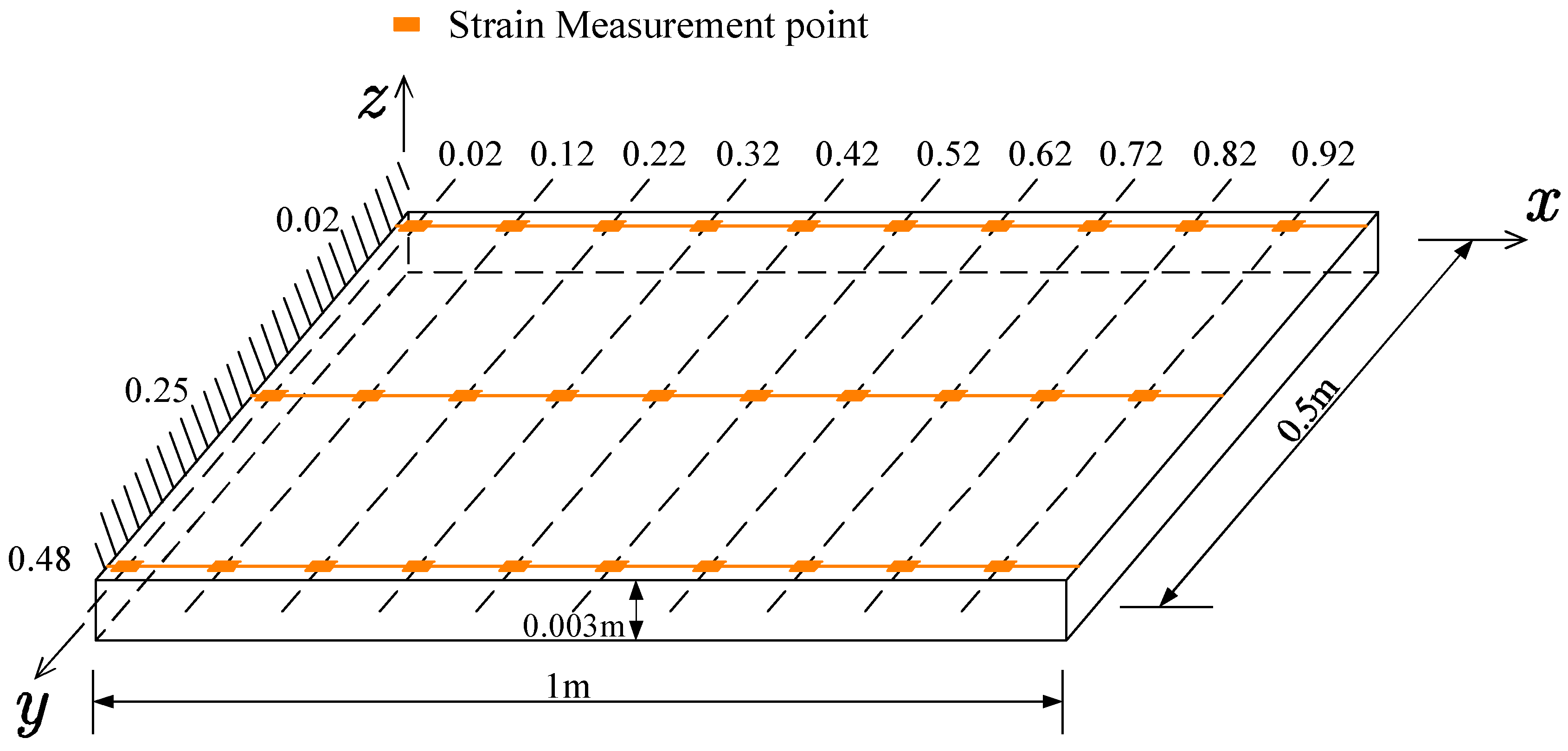
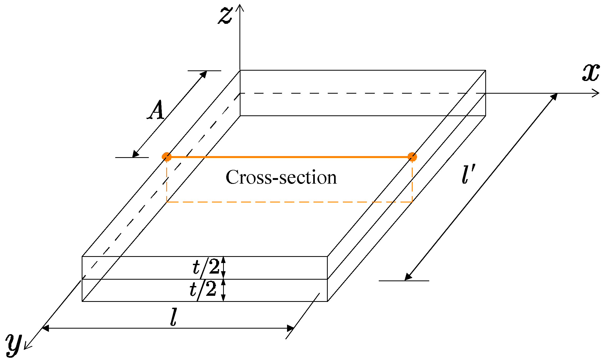
Figure 2.
Cartesian coordinate system used for the plate analysis.
Figure 2.
Cartesian coordinate system used for the plate analysis.
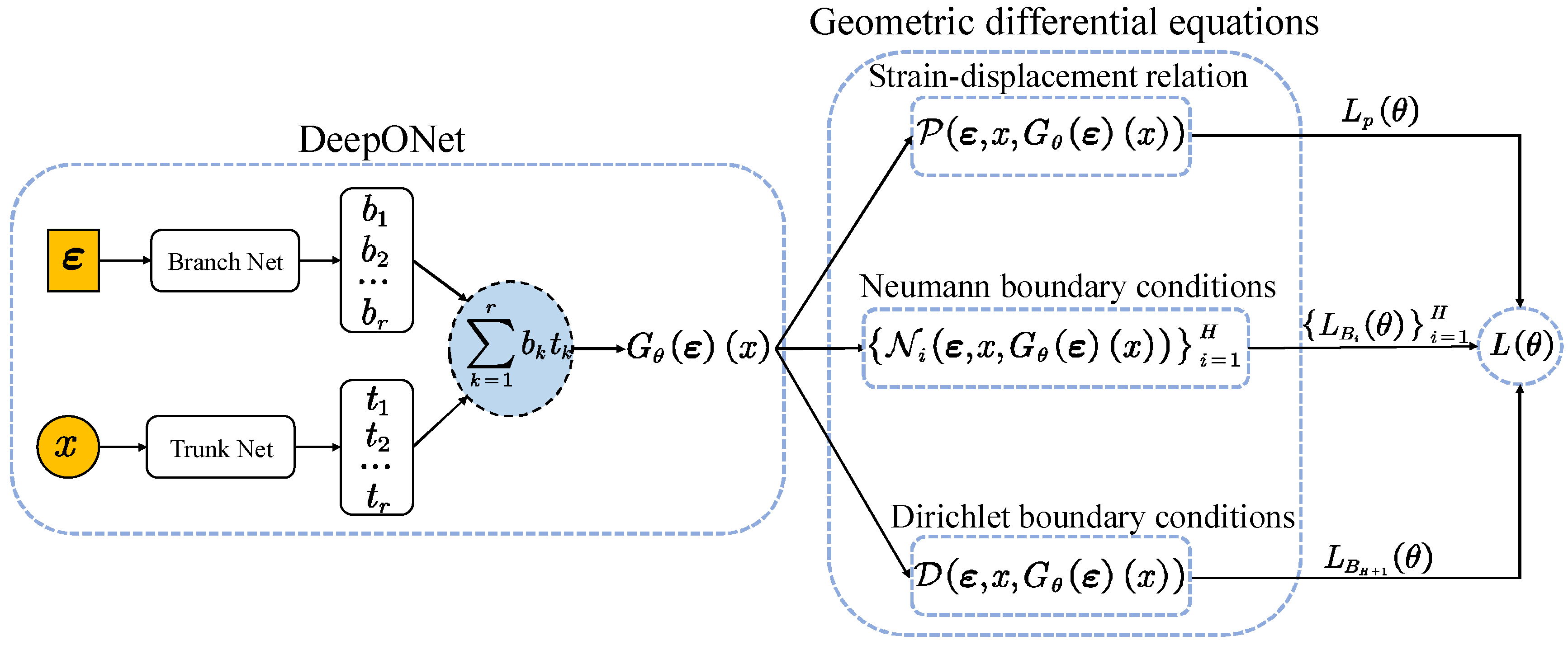
Figure 3.
Architecture of physics-informed DeepONet regularizing geometric differential equations.
Figure 3.
Architecture of physics-informed DeepONet regularizing geometric differential equations.
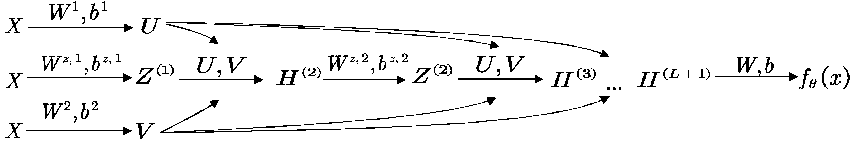
Figure 4.
Architecture of the new network serving as the trunk net and branch net.
Figure 4.
Architecture of the new network serving as the trunk net and branch net.
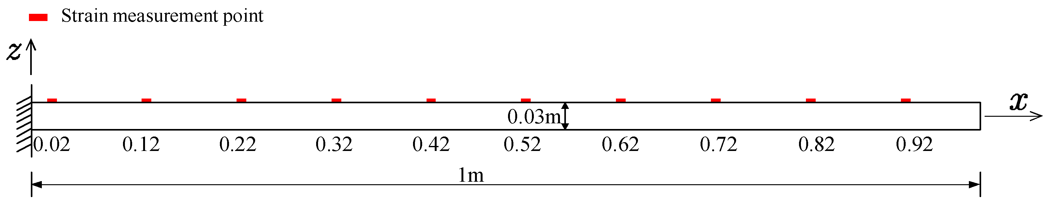
Figure 5.
The geometric model of the beam with one end clamped.
Figure 5.
The geometric model of the beam with one end clamped.
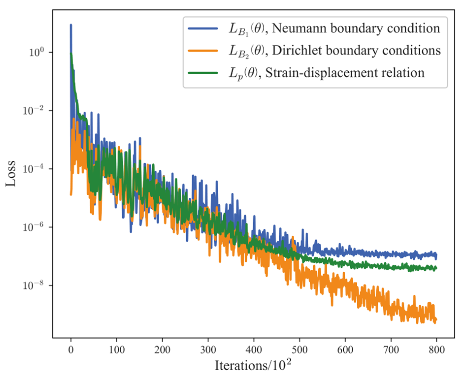
Figure 6.
Convergence process of each loss when training the PI_DeepONet for the beam with one end clamped.
Figure 6.
Convergence process of each loss when training the PI_DeepONet for the beam with one end clamped.
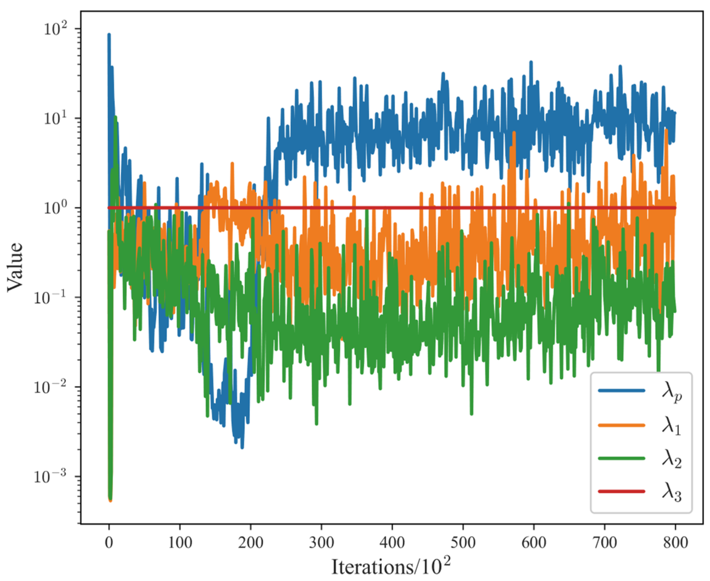
Figure 7.
Convergent evolution of the weight of the each physics-driven loss when training the PI_DeepONet for the beam with two ends clamped using Algorithm 1: denotes the weight of loss of strain–displacement relation, and denote the weights of the loss of Neumann boundary conditions at point = 0 m and = 1 m, respectively, and denotes the weight of the loss of Dirichlet boundary conditions.
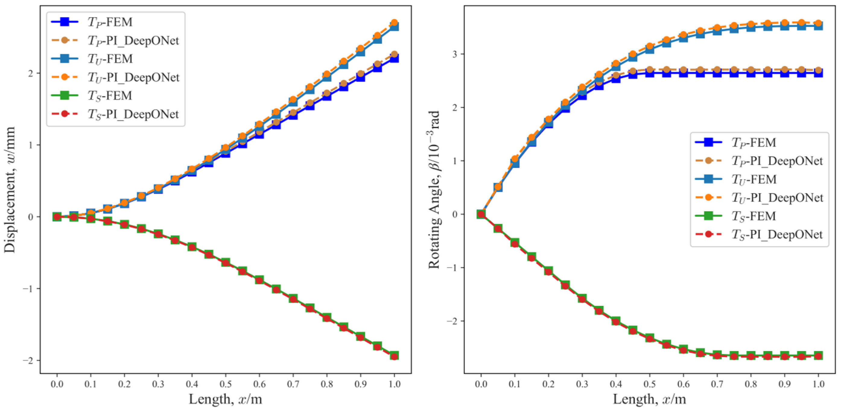
Figure 8.
Reconstruction results of the displacement and rotating angle of the beam with one end clamped under different loading conditions.
Figure 8.
Reconstruction results of the displacement and rotating angle of the beam with one end clamped under different loading conditions.
Figure 9.
Reconstruction results of the displacement and rotating angle of the beam with the restrictions of simply supported–simply supported under different loading conditions.
Figure 9.
Reconstruction results of the displacement and rotating angle of the beam with the restrictions of simply supported–simply supported under different loading conditions.
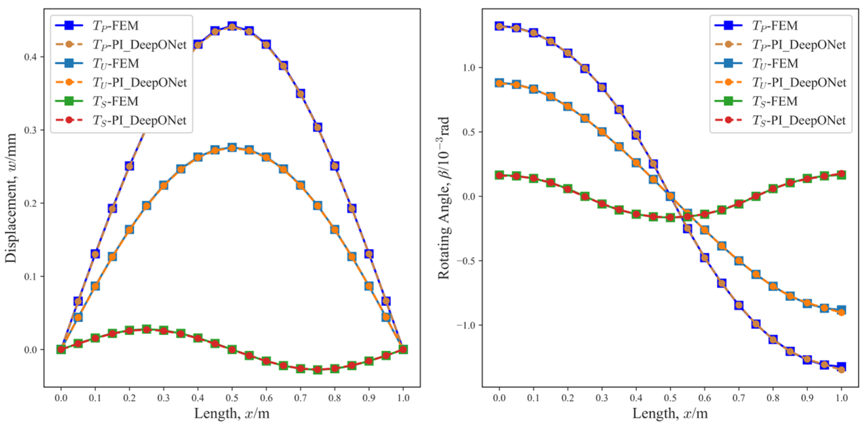
Figure 10.
Reconstruction results of the displacement and rotating angle of the beam with the restrictions of clamped–simply supported under different loading conditions.
Figure 10.
Reconstruction results of the displacement and rotating angle of the beam with the restrictions of clamped–simply supported under different loading conditions.
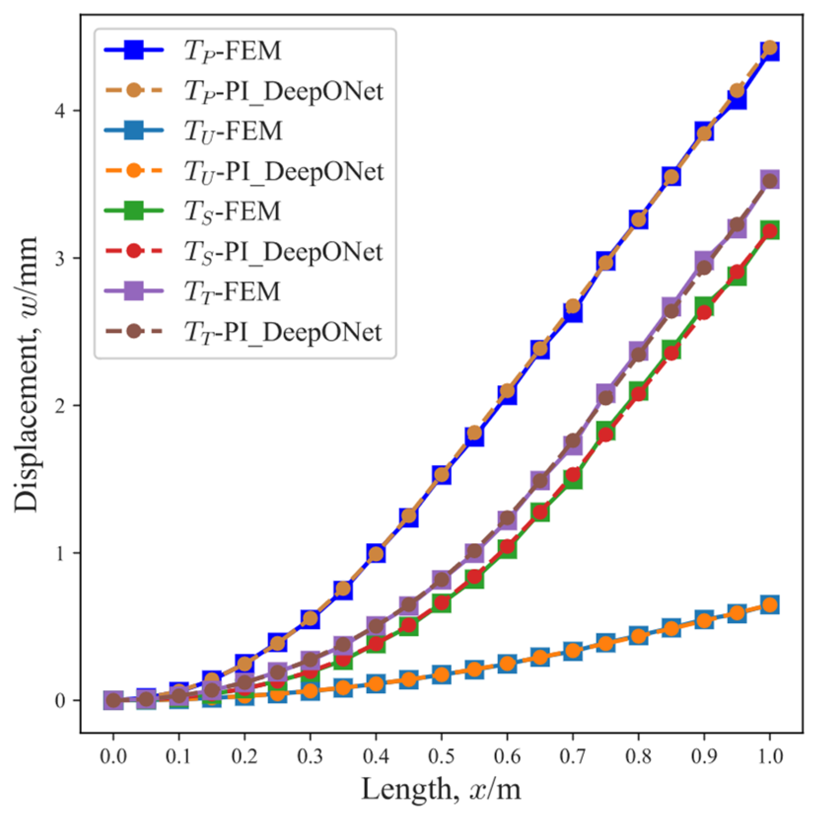
Figure 11.
Reconstruction results of the displacement and rotating angle of the beam with the restrictions of clamped–clamped under different loading conditions.
Figure 11.
Reconstruction results of the displacement and rotating angle of the beam with the restrictions of clamped–clamped under different loading conditions.
Figure 12.
Geometric model of the multi-span beam with the restrictions of clamped–simply supported–clamped.
Figure 12.
Geometric model of the multi-span beam with the restrictions of clamped–simply supported–clamped.
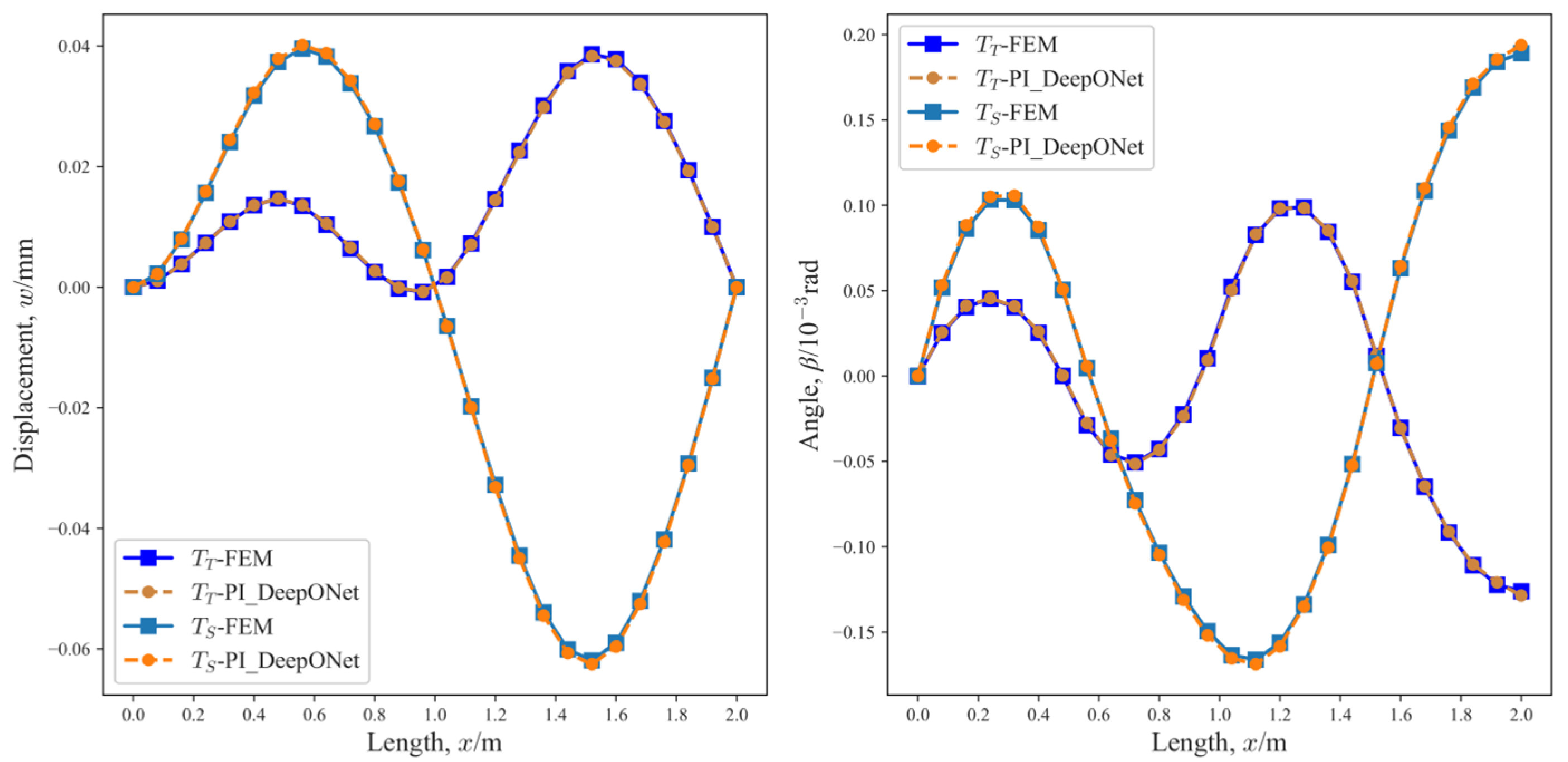
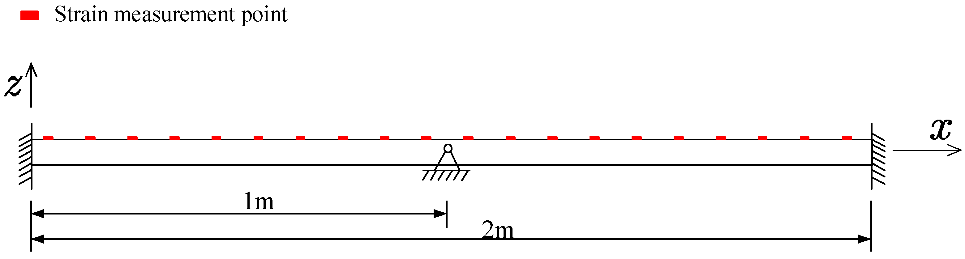
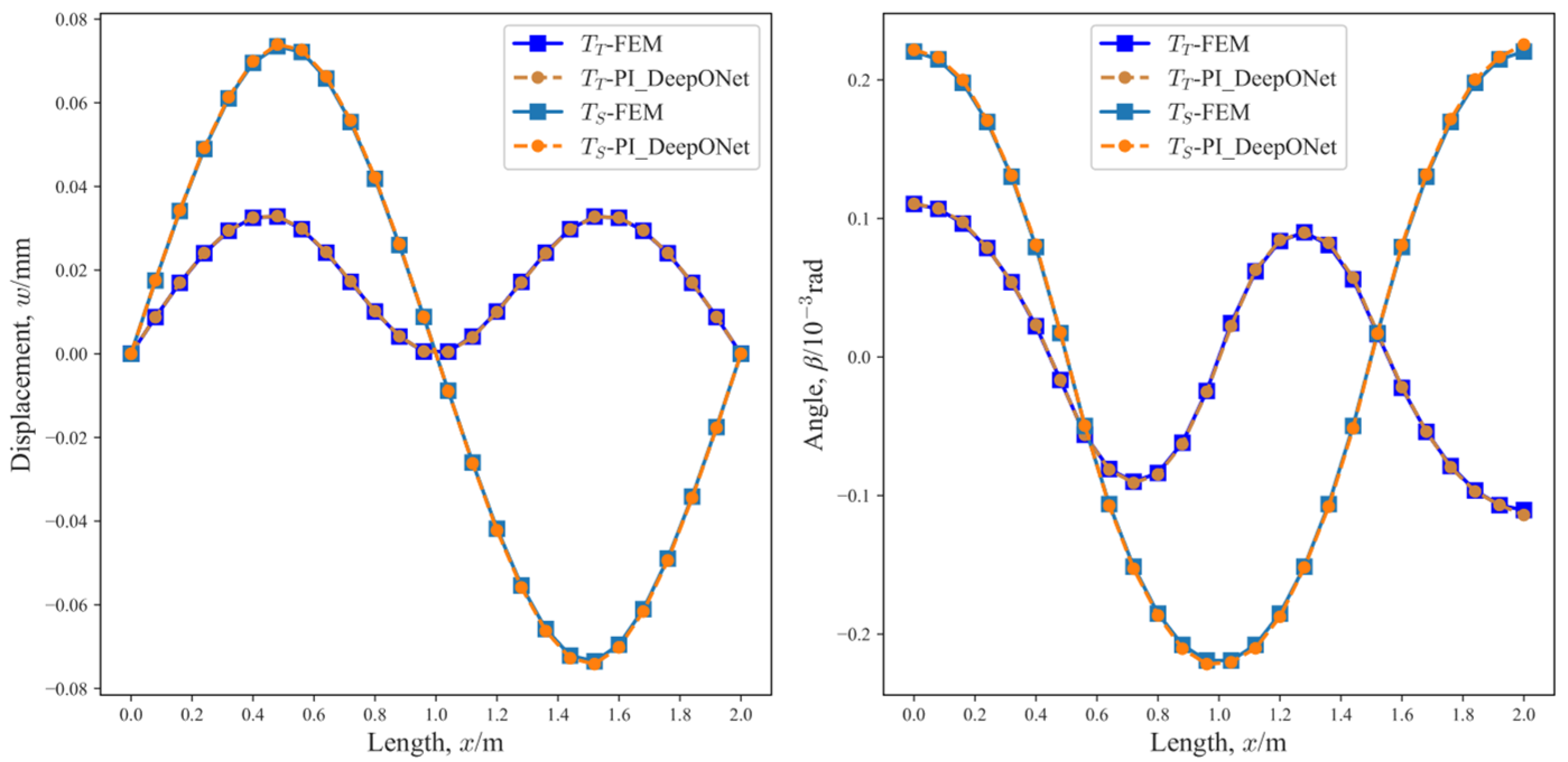
Figure 13.
Reconstruction results of the displacement and rotating angle of the multi-span beam with the restrictions of clamped–simply supported–clamped.
Figure 13.
Reconstruction results of the displacement and rotating angle of the multi-span beam with the restrictions of clamped–simply supported–clamped.
Figure 14.
Reconstruction results of the displacement and rotating angle of the multi-span beam with the restrictions of clamped–simply supported–simply supported.
Figure 14.
Reconstruction results of the displacement and rotating angle of the multi-span beam with the restrictions of clamped–simply supported–simply supported.
Figure 15.
Reconstruction results of the displacement and rotating angle of the multi-span beam with the restrictions of three points simply supported.
Figure 15.
Reconstruction results of the displacement and rotating angle of the multi-span beam with the restrictions of three points simply supported.
Figure 16.
The geometric model of the plate with one side clamped.
Figure 16.
The geometric model of the plate with one side clamped.
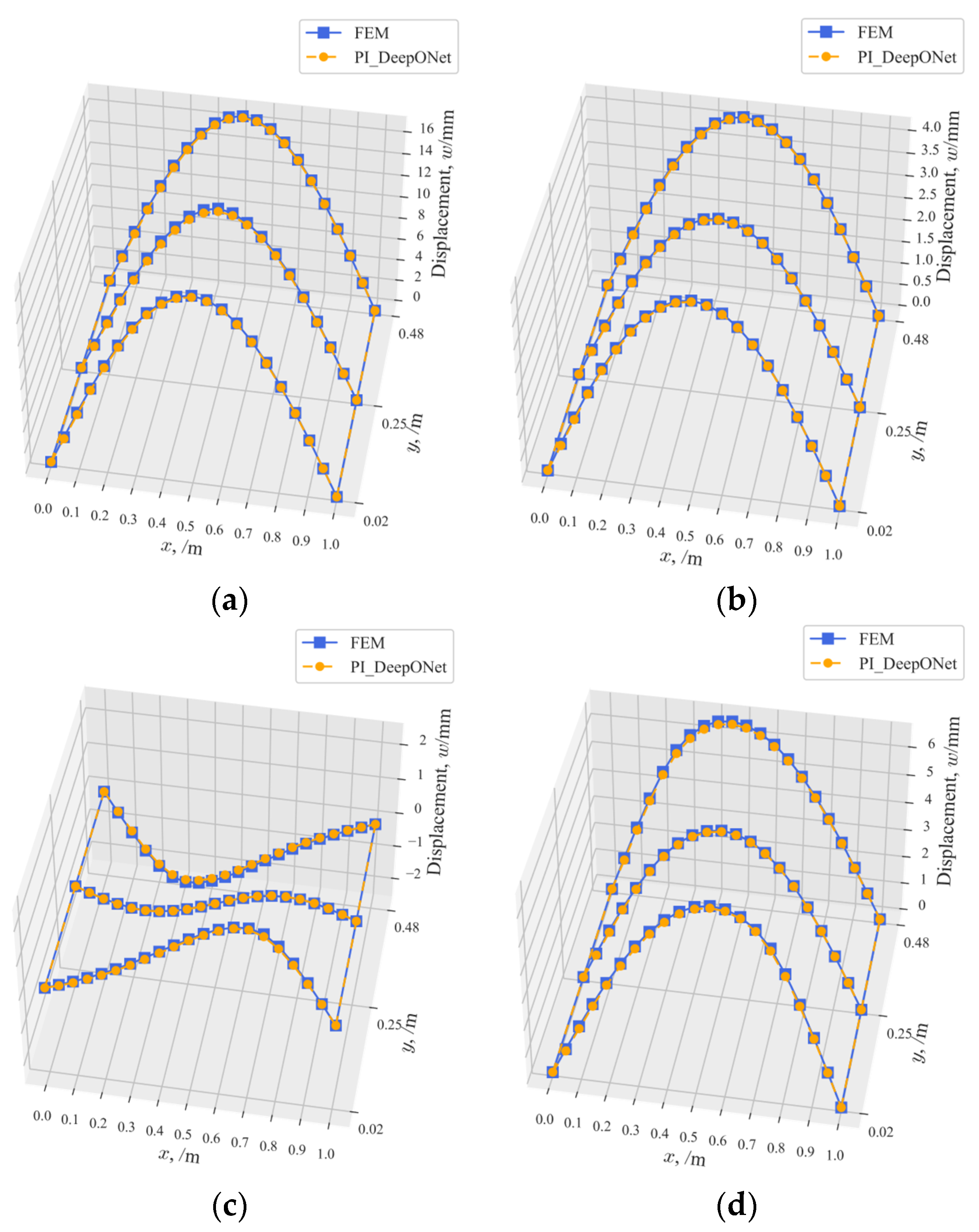
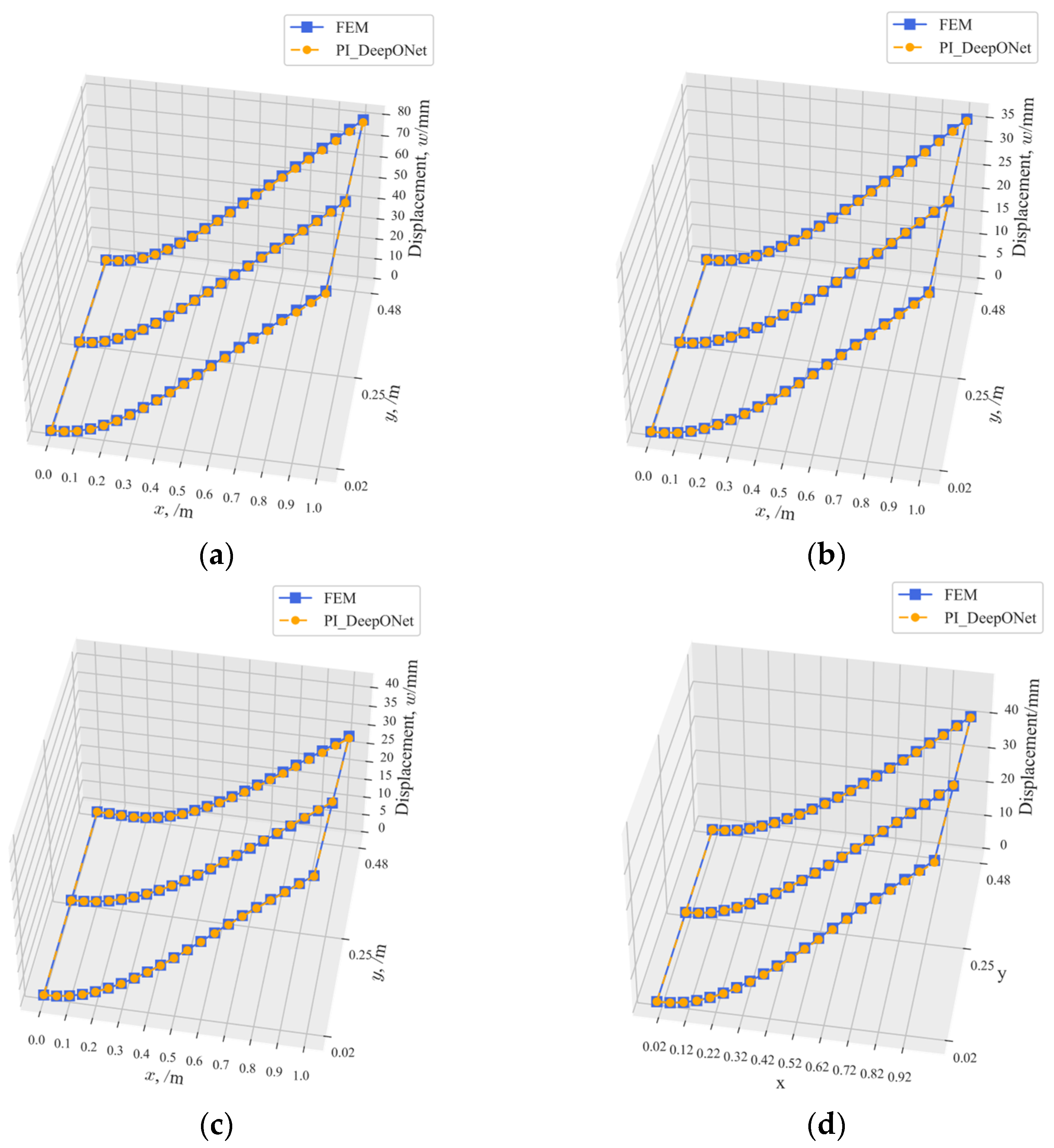
Figure 17.
Reconstruction results of the displacement for the plate with one side clamped under different loading conditions: (a) reconstruction results under loading condition , (b) reconstruction results under loading condition , (c) reconstruction results under loading condition , and (d) reconstruction results under loading condition .
Figure 18.
Reconstruction results of the displacement for the plate with two sides simply supported under different loading conditions: (a) reconstruction results under loading condition , (b) reconstruction results under loading condition , (c) reconstruction results under loading condition , and (d) reconstruction results under loading condition .
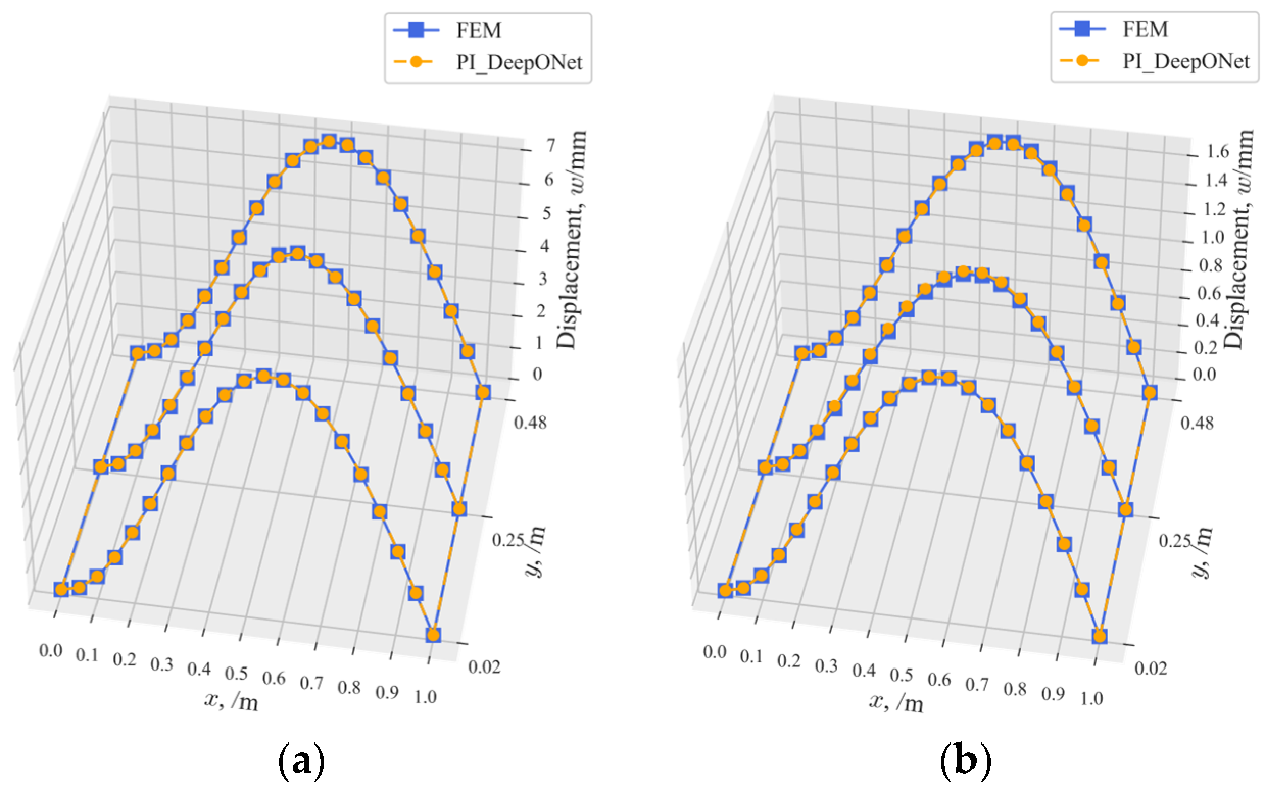
Figure 19.
Reconstruction results of the displacement for the plate with one side clamped and one side simply supported under different loading conditions: (a) reconstruction results under loading condition , (b) reconstruction results under loading condition , (c) reconstruction results under loading condition , and (d) reconstruction results under loading condition .
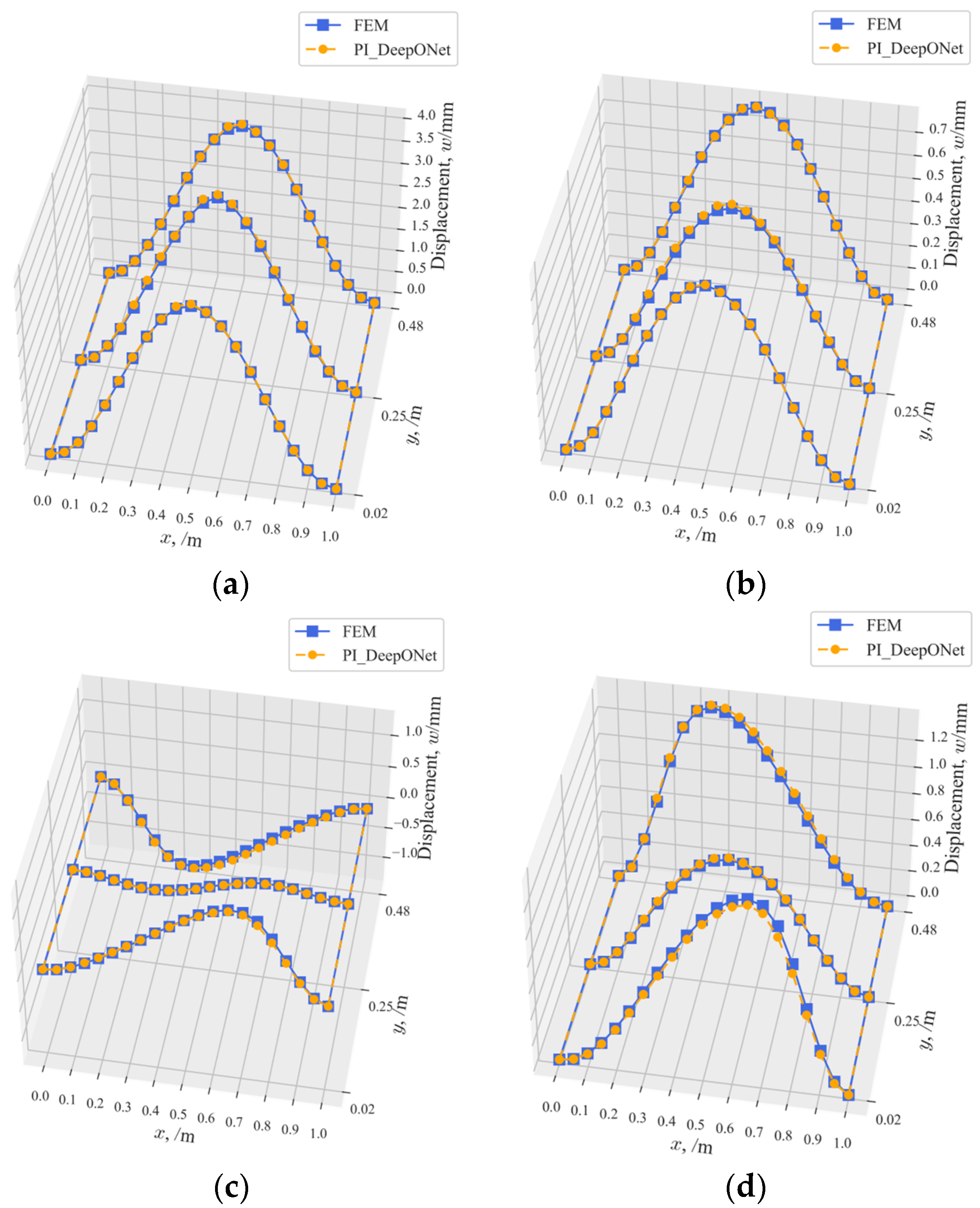
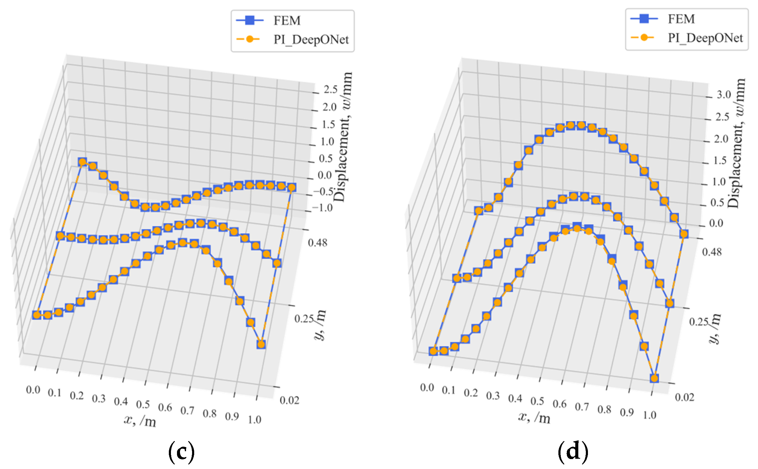
Figure 20.
Reconstruction results of the displacement for the plate with two sides clamped under different loading conditions: (a) reconstruction results under loading condition , (b) reconstruction results under loading condition , (c) reconstruction results under loading condition , and (d) reconstruction results under loading condition .
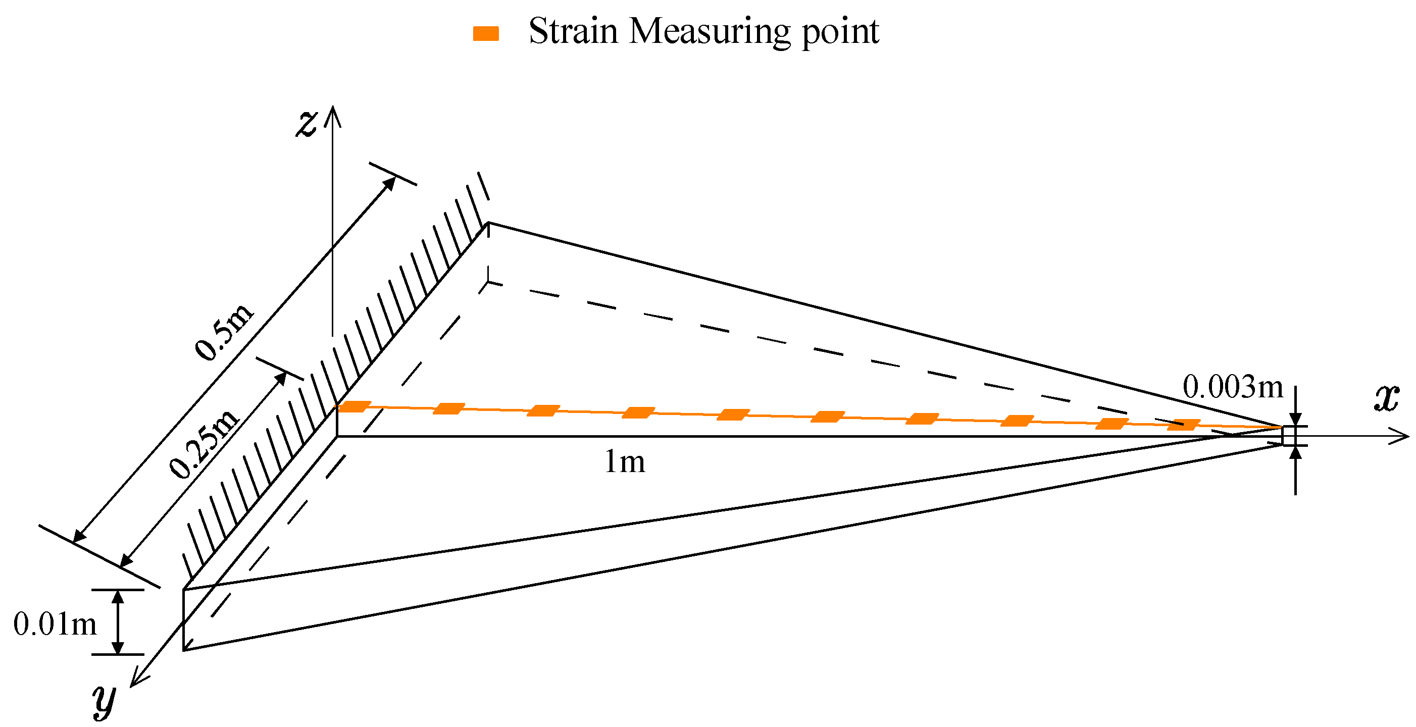
Figure 21.
The geometric model of the cantilevered triangle plate with variable cross-section.
Figure 21.
The geometric model of the cantilevered triangle plate with variable cross-section.
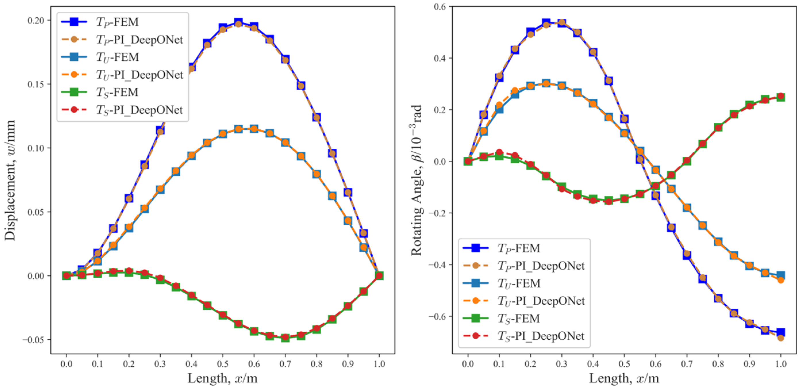
Figure 22.
Reconstruction results of the displacement for the triangle plate with variable thickness.
Figure 22.
Reconstruction results of the displacement for the triangle plate with variable thickness.
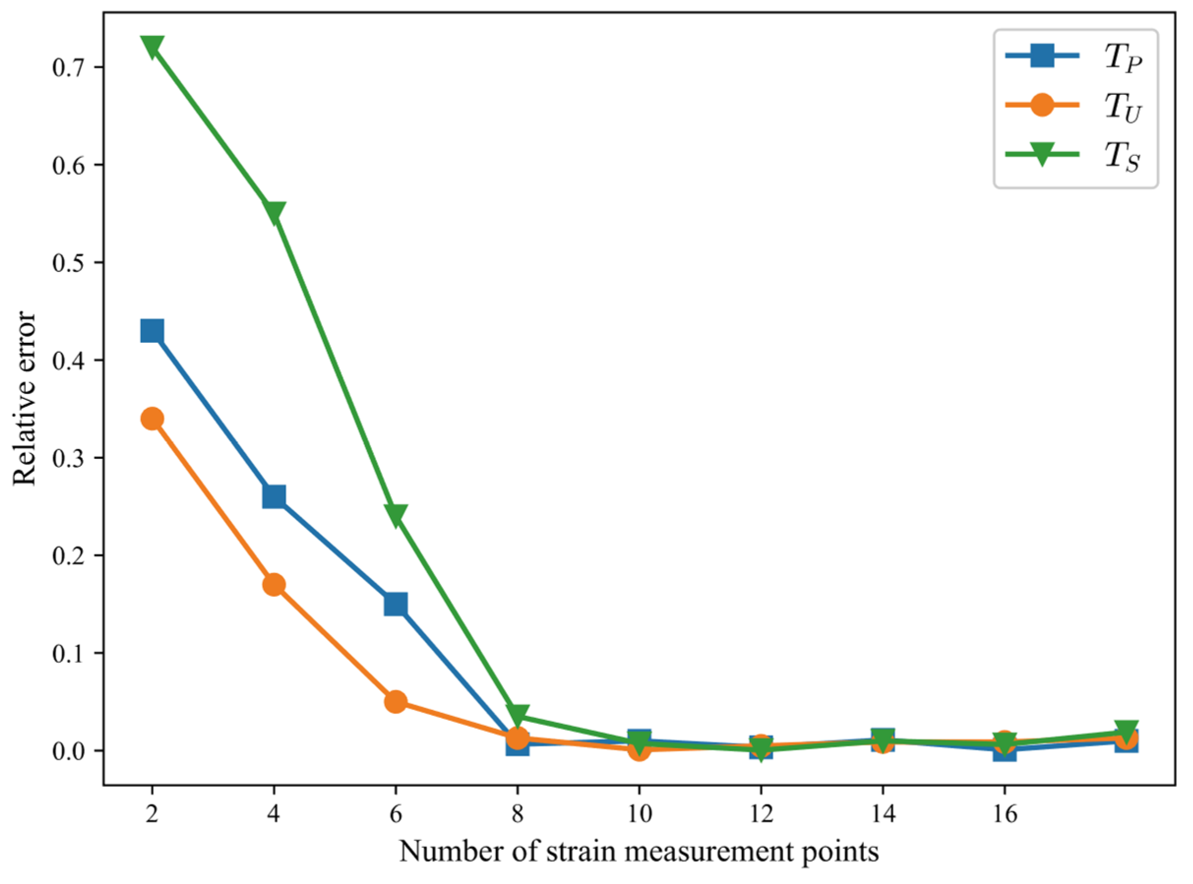
Figure 23.
Evolution of the relative error at the maximum response with the number of strain measurement points for the beam with the restriction of two clamped ends.
Figure 23.
Evolution of the relative error at the maximum response with the number of strain measurement points for the beam with the restriction of two clamped ends.
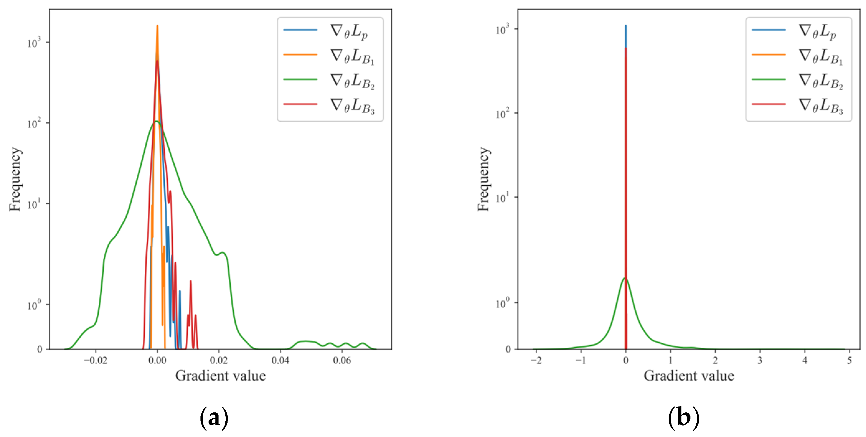
Figure 24.
Histograms of back-propagated gradients of each physics-driven loss for the beam with restrictions of clamped–clamped at the first layer of the trunk net after 40,000 training iterations of a PI_DeepONet: (a) histograms of back-propagated gradients with the updated weights applied and (b) histograms of back-propagated gradients with all weights set as 1.
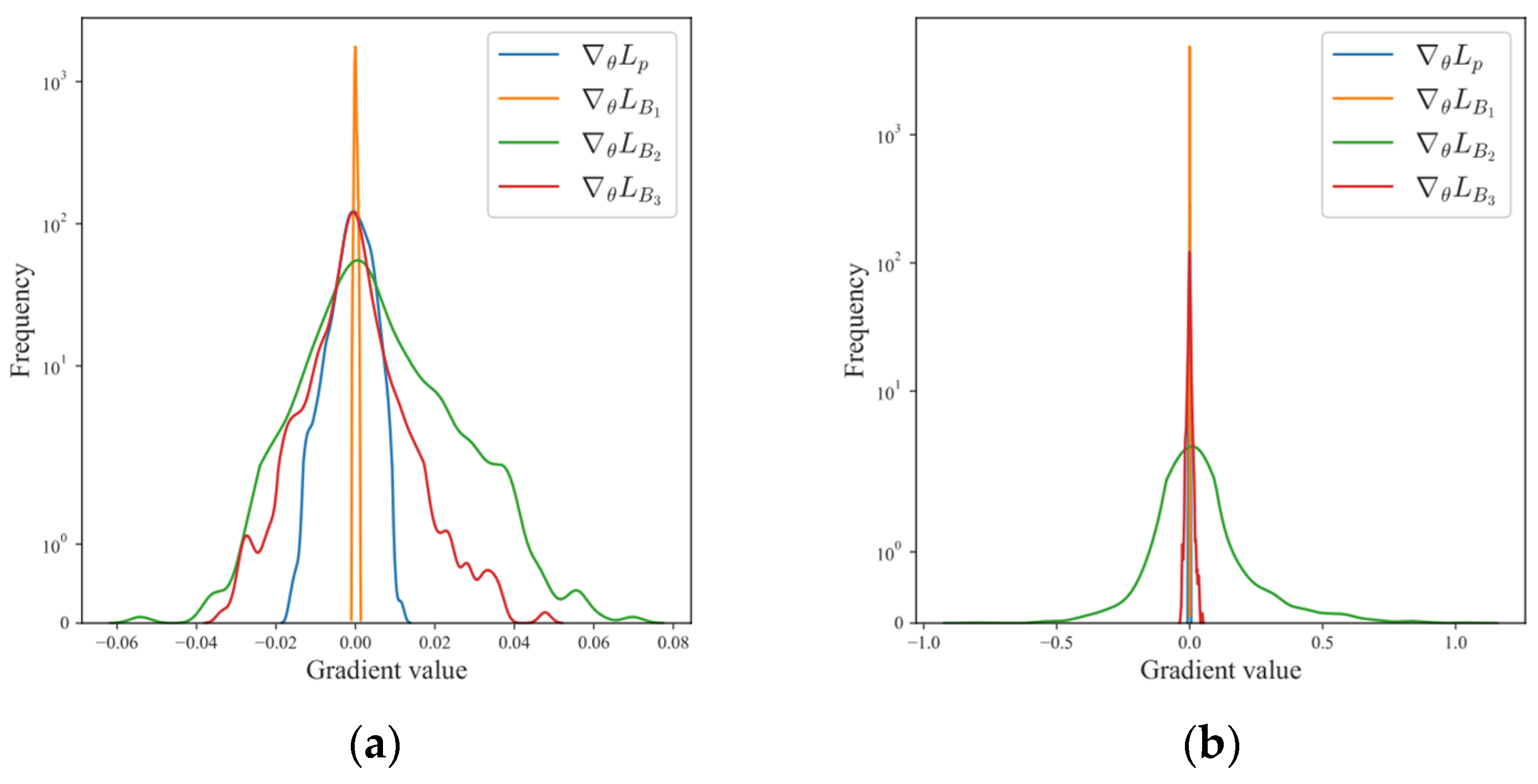
Figure 25.
Histograms of back-propagated gradients of each physics-driven loss for the multi-span beam with the restrictions of clamped–simply supported–clamped at the first layer of trunk net after 40,000 iterations of training for PI_DeepONet: (a) histograms of back-propagated gradients with the updated weights applied and (b) histograms of back-propagated gradients with all weights set as 1.
Figure 26.
Histograms of back-propagated gradients of each physics-driven loss for the plate with the restrictions of clamped–clamped at the first layer of trunk net after 40,000 iterations of training PI_DeepONet: (a) histograms of back-propagated gradients with the updated weights applied and (b) histograms of back-propagated gradients with all weights set as 1.
Table 1.
Boundary conditions for different restrictions.
Table 1.
Boundary conditions for different restrictions.
| Restriction | Boundary Conditions |
|---|
| Free | or are not specified |
| Simply supported | |
| Clamped | |
Table 2.
Loads applied to the beam.
Table 2.
Loads applied to the beam.
| Loading Conditions | Magnitude and Position of Each Load |
|---|
| Point load | 300 N at = 0.5 m |
| Uniform pressure | 0.01 Mpa on the upper surface of the beam |
| Staggered load | 150 N at = 0.25 m; −150 N at = 0.75 m |
Table 3.
Fitting accuracy of the PI_DeepONet for the beam.
Table 3.
Fitting accuracy of the PI_DeepONet for the beam.
| Restrictions | Displacement Fitting Accuracy | Rotating Angle Fitting Accuracy |
|---|
| | | | | |
|---|
| one end clamped | 0.9979 | 0.9984 | 0.9996 | 0.9937 | 0.9965 | 0.9993 |
| simply supported–simply supported | 0.9999 | 0.9999 | 0.9996 | 0.9999 | 0.9999 | 0.9993 |
| clamped–simply supported | 0.9997 | 0.9998 | 0.9979 | 0.9997 | 0.9992 | 0.9959 |
| clamped–clamped | 0.9998 | 0.9999 | 0.9962 | 0.9997 | 0.9995 | 0.9973 |
Table 4.
Loads applied to the multi-span beam.
Table 4.
Loads applied to the multi-span beam.
| Loading Conditions | Magnitude and Position of Each Load |
|---|
| Two-point loads | 5 N at = 0.5 m; 5 N at = 1.5 m |
| Staggered load | 5 N at = 0.5 m; −5 N at = 1.5 m |
Table 5.
Fitting accuracy of the PI_DeepONet for the multi-span beam.
Table 5.
Fitting accuracy of the PI_DeepONet for the multi-span beam.
| Restrictions | Displacement Fitting Accuracy | Rotating Angle Fitting Accuracy |
|---|
| | | |
|---|
| clamped–simply supported–clamped | 0.9983 | 0.9999 | 0.9986 | 0.9994 |
| clamped–simply supported–simply supported | 0.9998 | 0.9998 | 0.9998 | 0.9997 |
| three points simply supported | 0.9999 | 0.9999 | 0.9998 | 0.9998 |
Table 6.
Loads applied to the plate.
Table 6.
Loads applied to the plate.
| Loading Conditions | Magnitude and Position of Each Load |
|---|
| Point load | 200 N at ( = 0.5 m, = 0.25 m) |
| Uniform pressure | 150 Pa on the upper surface |
| Staggered loads | 50 N at ( = 0.75 m, = 0 m); −50 N at ( = 0.25 m, = 0.5 m) |
| Two-points loads | 50 N at ( = 0.75 m, = 0 m); 50 N at ( = 0.25 m, = 0.5 m) |
Table 7.
Fitting accuracy of the PI_DeepONet for the plate.
Table 7.
Fitting accuracy of the PI_DeepONet for the plate.
| Restrictions | Displacement Fitting Accuracy |
|---|
| | | |
|---|
| one side clamped | 0.9995 | 0.9996 | 0.9996 | 0.9997 |
| simply supported–simply supported | 0.9991 | 0.9995 | 0.9991 | 0.9989 |
| clamped–simply supported | 0.9999 | 0.9996 | 0.9997 | 0.9994 |
| clamped–clamped | 0.9995 | 0.9993 | 0.9984 | 0.9966 |
Table 8.
Loads applied to the triangle plate with variable thickness.
Table 8.
Loads applied to the triangle plate with variable thickness.
| Loading Conditions | Magnitude and Position of Each Load |
|---|
| Point load | 100 N at (= 0.5 m, = 0 m) |
| Uniform pressure | 150 Pa on the upper surface |
| Staggered loads | 50 N at ( = 0.75 m, = −0.0625 m); −50 N at ( = 0.25 m, = 0.1875 m) |
| Two-point loads | 50 N at ( = 0.75 m, = −0.0625 m); 50 N at ( = 0.25 m, = 0.1875 m) |
Table 9.
Fitting accuracy of the PI_DeepONet for the triangle plate with variable thickness.
Table 9.
Fitting accuracy of the PI_DeepONet for the triangle plate with variable thickness.
| Loading Conditions | Displacement Fitting Accuracy |
|---|
| Point load | 0.9999 |
| Uniform load | 0.9997 |
| Staggered load | 0.9998 |
| Two points | 0.9997 |
Table 10.
Relative errors in the maximum response calculated by the PI_DeepONet via uniformly arranged measurement points and randomly arranged measurement points for the beam with different restrictions.
Table 10.
Relative errors in the maximum response calculated by the PI_DeepONet via uniformly arranged measurement points and randomly arranged measurement points for the beam with different restrictions.
| Restrictions | Relative Errors |
|---|
| Uniformly Arranged Strain Measurement Points | Randomly Arranged Strain Measurement Points |
|---|
| | | | | |
|---|
| one end clamped | 2.5% | 2.2% | 1.0% | 2.7% | 1.4% | 0.055% |
| simply supported–simply supported | 0.32% | 0.29% | 2.9% | 0.78% | 0.013% | 1.1% |
| clamped–simply supported | 0.78% | 0.013% | 1.7% | 1.1% | 0.024% | 1.3% |
| clamped–clamped | 1.0% | 0.088% | 0.74% | 0.30% | 0.44% | 1.1% |
Table 11.
Relative errors at the maximum response calculated by the PI_DeepONet for the beam with the restrictions of clamped–clamped.
Table 11.
Relative errors at the maximum response calculated by the PI_DeepONet for the beam with the restrictions of clamped–clamped.
| Method | Relative Errors |
|---|
| | |
|---|
| Algorithm 1 | 1.6% | 0.64% | 3.7% |
| Gaussian probabilistic models | 1.0% | 3.4% | 33% |
| Normal gradient descent iterations | 31% | 40% | 55% |
Table 12.
Relative errors at the maximum response calculated by the PI_DeepONet for the multi-span beam with the restrictions of clamped–simply supported–clamped.
Table 12.
Relative errors at the maximum response calculated by the PI_DeepONet for the multi-span beam with the restrictions of clamped–simply supported–clamped.
| Method | Relative Errors |
|---|
| |
|---|
| Algorithm 1 | 1.9% | 0.35% |
| Gaussian probabilistic models | 2.8% | 2.5% |
| Normal gradient descent iterations | 6.1% | 3.9% |
Table 13.
Relative errors at the maximum response calculated by the PI_DeepONet for the plate with the restrictions of clamped–clamped.
Table 13.
Relative errors at the maximum response calculated by the PI_DeepONet for the plate with the restrictions of clamped–clamped.
| Method | Relative Errors |
|---|
| | | |
|---|
| Algorithm 1 | 1.3% | 0.026% | 2.0% | 3.2% |
| Gaussian probabilistic models | 27% | 26% | 64% | 57% |
| Normal gradient descent iterations | 9.2% | 6.7% | 4.2% | 21% |
Table 14.
Relative errors at the maximum response calculated by the PI_DeepONet and Ko method for the beam with the restrictions of clamped–clamped.
Table 14.
Relative errors at the maximum response calculated by the PI_DeepONet and Ko method for the beam with the restrictions of clamped–clamped.
| Method | Relative Errors |
|---|
| | |
|---|
| PI_DeepONet | 0.9% | 1.0% | 3.7% |
| Ko method | 0.9% | 5.6% | 13% |


 ,
, 


