Efficient Modulation Recognition by Predictive Correction and Double GRUs via a Lightweight Framework

Abstract

Automatic modulation recognition (AMR) provides excellent performance advantages over conventional algorithms and plays a key role in modern communication. However, a general challenge is that the channel errors greatly deteriorate the classification capability, and the computational complexity is extremely high. To reduce the offset error of the signal and ensure fewer parameters to save training resources, we demonstrated an efficient modulation recognition scheme combined predictive correction with double Gate Recurrent Unit (GRU), thus realizing a lightweight neural framework. Predictive correction reduces channel errors, and double GRUs are better at capturing long-term dependencies. The results show that when the signal-to-noise ratio is around 18 dB, the highest recognition accuracy can be achieved, and the computational complexity is significantly reduced. The proposed scheme exhibits a tradeoff between the accuracy and the computational complexity, providing an attractive method for modulation recognition.

1. Introduction

Automatic modulation recognition (AMR) has grown in significance in wireless communication [1]. AMR methods mainly included likelihood-based (LB) and feature-based (FB) [2]. The LB method requires complex computation to calculate the comparison for recognition [3]. The FB method needs to design classifiers such as Support Vector Machines (SVM) [4], Decision Trees (DT) [5], artificial neural networks [6], etc. In recent years, with the development of Deep Learning (DL), it has a good ability of classification, induction and migration, and has made a major breakthrough in the field of signal modulation recognition [7]. In 2016, O’Shea et al. used a 2 × 128 matrix as input to a convolutional neural network for the first time to recognize 11 modulated signals. In the following year, the recognition of 24 modulated signals was completed by using residual neural network and other methods [8,9,10]. CNN algorithms solely took into account the signal’s spatial characteristics, ignoring its temporal properties [11]. Xu used the temporal characteristics of the signal that were taken out of the unidirectional Recurrent Neural Network (RNN) [12], but this technique ignores the problem of the signal being distorted by offset interference. In order to reduce the influence of carrier frequency and phase offset on modulation recognition, a learnable offset correction model can improve classification accuracy and correct channel errors [13]. However, this scheme only considers the combination with CNN, resulting in too large parameters. Zhang et al. combined learnable correction modules with CNN and Gated Recursive Units (GRUs) to make lightweight improvements [14]. To obtain a reasonable tradeoff between classification accuracy and computational complexity, we propose an efficient DL-AMR scheme using predictive correction combined with double GRUs via a lightweight framework. After error learning and estimation, the signal is restored by inverse transformation to realize signal correction, and after that, CNN and two GRU layers are used to extract the spatial and temporal characteristics for classification. This method not only improves the recognition accuracy, but also achieves low computational complexity.

2. System Framework

The signal sampled passes through the channel and can be articulated as:

$$y[l]=A[l]e^{j(\omega l+\phi )}x[l]+n[l],l=1,\dots ,L$$

(1)

where the complex Additive White Gaussian Noise (AWGN) is denoted by n[l] and x[l] is the signal that the transmitter has modulated using a particular modulation method. The channel gain is represented by A[l], where ω and φ, respectively, stand for the frequency and phase offset. The number of symbols in a signal sample is represented by L, which can be represented as follows. In-phase/quadrature (I/Q) form, which is represented as follows, can be recorded for the received signals:

$$y=[\Re \{y[1]\},\dots ,\Re \{y[L]\};\Im \{y[1]\},\dots ,\Im \{y[L]\}]$$

(2)

The offset interference received by the signal in the channel mainly includes frequency offset and phase offset. Different signals contain different frequency components, and different arrival times will lead to a phase offset. Frequency deviation between transmitter and receiver and instability of frequency oscillator result in frequency offset. The constellation diagram of QPSK signal makes it easy to observe changes directly. Select a group of constellation diagrams of the signal at 18 dB to see the impact of frequency offset and phase offset on the signal. It can be seen from Figure 1 that when the signal is not affected, it is correctly represented on the constellation diagram. When the phase offset is 30° and the frequency offset is 400 Hz, the rotation dispersion changes obviously; when the phase offset is 60° and the frequency offset is 800 Hz, the changes in the constellation diagram are more obvious. The above changes can be approximately summarized as offset, rotation, and scaling.

GRU is a variant of RNN, which mainly combines the forget gate and input gate into a single update gate. The GRU model is simpler than the standard RNN model. Its effect is similar to RNN, but the parameters are reduced, such that it is not easy to overfit.

To eliminate errors of the channel reception, as shown in Part A of Figure 2, the predictive correction module is introduced. The sampled I/Q data are altered by channel noise and interference, leading to phenomena like temporal shifting, linear mixing, and spinning of the received signal. In order to eliminate channel reception errors and reduce the training cost, a learnable predictive correction model is shown in Figure 2, which includes Part A and double-layers GRU convolutional neural network noted by Part B.

By co-training with the subsequent model, the Part A predictive correction model may estimate the parameters. These parameters are learned from the effects of frequency offset, phase offset, time drift, and noise on the signal, which can be represented as position information carried by frequency offsets and phase offsets. Two dense layers and a flatten layer can each learn phase and frequency offset information for every 128 × 2 I/Q sample. After the flatten layer flattens the input signal y into a vector to match the input dimension of the dense layer, the data traveling through the layer give the offset parameters. The dense layer’s linear activation function yields and estimates the offset parameter across an unlimited, continuous range. The original signal y can be multiplied to produce the corrected signal by the use of the offset parameter and inverse transformation, denoted as follows:

$$\widehat{y}[l]=y[l]e^{-j\widehat{\phi }}=\left[\begin{array}{c}\Re \{y[l]\}\cos \widehat{\phi }+\Im \{y[l]\}\sin \widehat{\phi }\\ \Im \{y[l]\}\cos \widehat{\phi }-\Re \{y[l]\}\sin \widehat{\phi }\end{array}\right]$$

(3)

$\widehat{y}$ = [$\widehat{y}$[1], …,$\widehat{y}$[L]],], which represents the correction signal. Part A learned positional information containing 6 parameters, including translation, rotation, and scaling transformation information, namely, the relationship between phase offset and frequency offset. Among the 6 parameters, the coordinates of each point after correction (x′, y′) can be articulated as follows:

$$\left[\begin{array}{l}{x}^{\prime }\hfill \\ y^{\prime }\hfill \end{array}\right]=\left[\begin{array}{ll}a\hfill & b\hfill \\ c\hfill & d\hfill \end{array}\right]\left[\begin{array}{l}x\hfill \\ y\hfill \end{array}\right]+\left[\begin{array}{l}e\hfill \\ f\hfill \end{array}\right]$$

(4)

The parameters a–d indicate the translation and rotation of the received signal, which can approximately express the impact of frequency offset. The e and f parameters indicate that the time shift can approximately express the effect of phase offset. Implementing a single correction only requires ω and φ maintaining the corresponding parameter changes. (x, y) represents the coordinates of each constellation point before correction.

CNN, two GRUs, and a thick layer that supports feature extraction and classification make up Part B. The signal’s spatial features are retrieved by the first convolution layer, which has 75 filters and a 2 × 8 kernel size. The extracted features are then further compressed by the second convolution layer, which has 25 filters and a 1 × 5 kernel size. The temporal characteristics of the signal are extracted using the following GRU layers using 40 units. Ultimately, the dense layer—which has the same number of modulation classes—completes the classification assignment. Repaired linear unit activation functions are used in the first two convolution layers, On the other hand, the final thick layer uses Softmax. In order to produce a model that is smaller and requires less computing power, the matching network in the third part is designed to control the model size using a restricted number of parameters in the CNN layers.

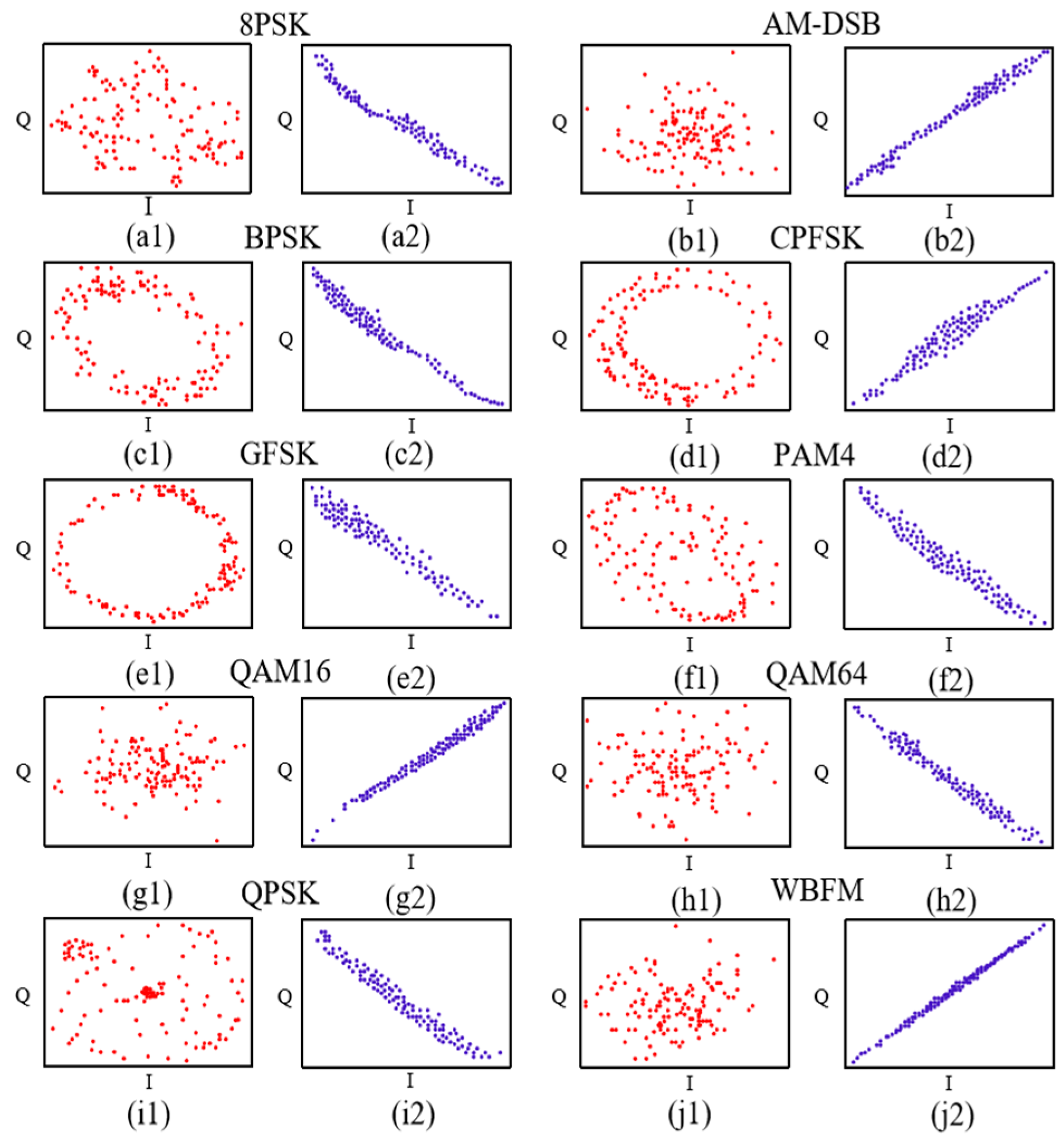
In order to confirm that the suggested approach is genuine, a comparative study was carried out to analyze the signal constellation maps without prediction correction and with the corrected ones when the signal SNR is set to be 10 dB, as shown in Figure 3.

The original dataset’s constellation diagram is shown on the left side of Figure 3, while the right side represents the improved constellation diagram of Part A output after offset correction. It can be seen that compared to the original signals, after introducing a correction process, the signals are tightly distributed and more conducive to GRUs extracted bidirectional of temporal features.

The RadioML2016.10b [15] experimental dataset, produced using the GNU Radio channel model, is generated by simulating the propagation properties in a harsh environment. The datasets included the same carrying data as the actual signal, as well as pulse shaping, modulation, and emission parameter characterization.

Table 1. Main parameter of RadioML2016.10b dataset.

Parameter	Value
Standard deviation is offset by sampling rate.	0.01 Hz
Maximum offset for sampling rate	50 Hz
Maximum offset for carrier frequency	500 Hz
Standard deviation of carrier frequency offset	0.01 Hz
Sample length	128
SNR range	−20 dB–18 dB
Sampling rate	200 kHz
Number of samples	1,200,000
Modulation modes	10

displays the parameters for the RadioML2016.10b datasets. There were 1,200,000 dataset samples in all, with ten distinct modulation types operating at twenty Signal-to-Noise Ratios (SNRs) and continuously balanced signal samples.

3. Results and Discussion

With random selection, the database is split into three sections: training, validation, and test, with a ratio of 6:2:2 for each class. The loss function is categorical cross-entropy, and Adam is the optimizer. The training procedure ends, and the training model is saved with the lowest validation loss when the validation loss does not drop after five epochs of multiplication by a coefficient of 0.5. The GeForce GTX1050 GPU and the experiments are implemented using Keras as the front end and Tensorflow as the back end.

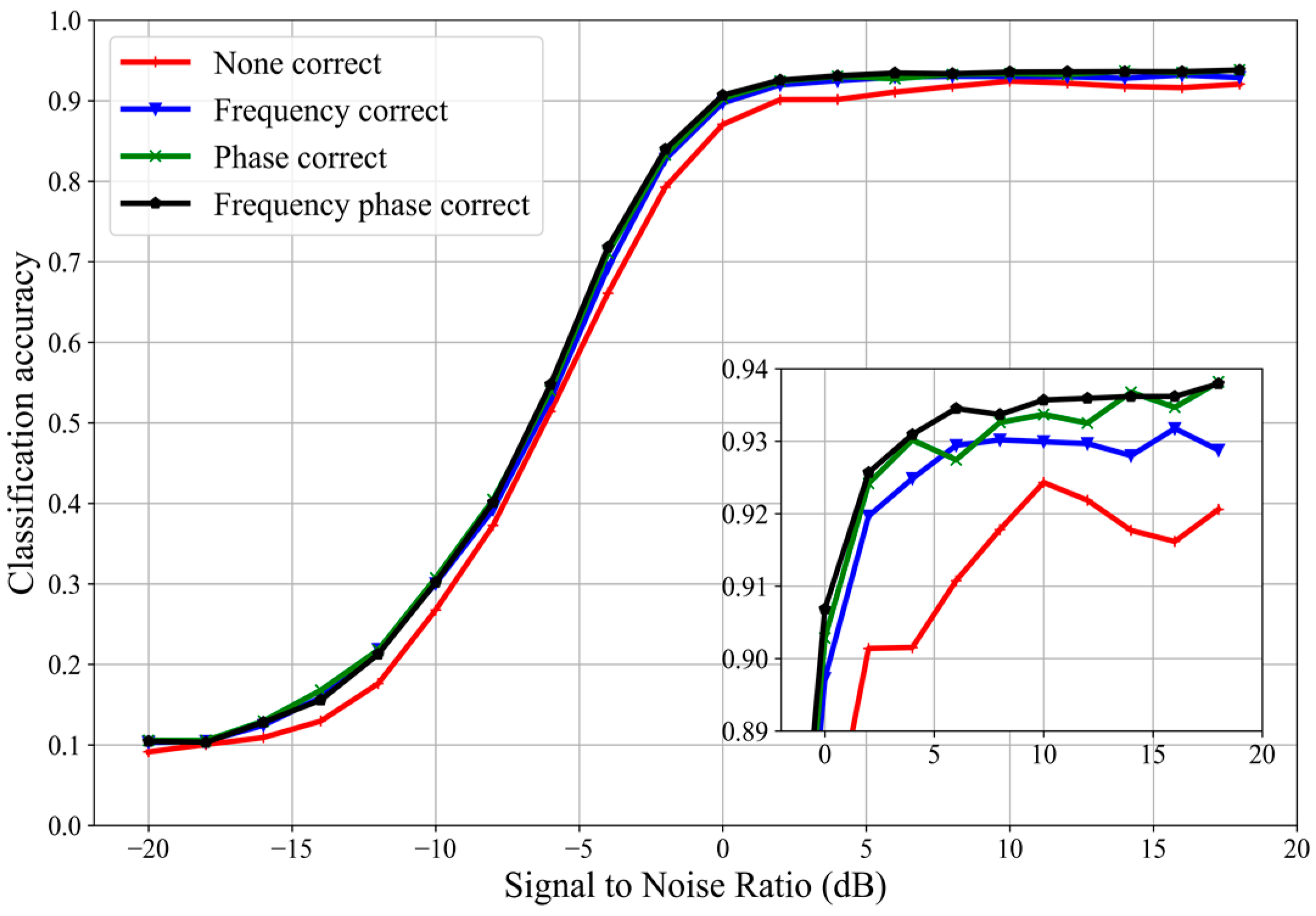
Further tests were carried out that produced definitive findings, even if it was a typical series of experiments to identify beneficial architectures and hyperparameter settings. We performed a contrast experiment to confirm the efficacy of phase and frequency correction in order to compare the efficiency of the suggested strategy. Four sets of comparison experiments were conducted, which were no correction, single frequency correction, single phase correction, and proposed frequency and phase correction method. The effect of frequency offset included the effect of phase offset. Figure 4 shows that the proposed method has better performance in recognition accuracy than the other three comparative experimental methods.

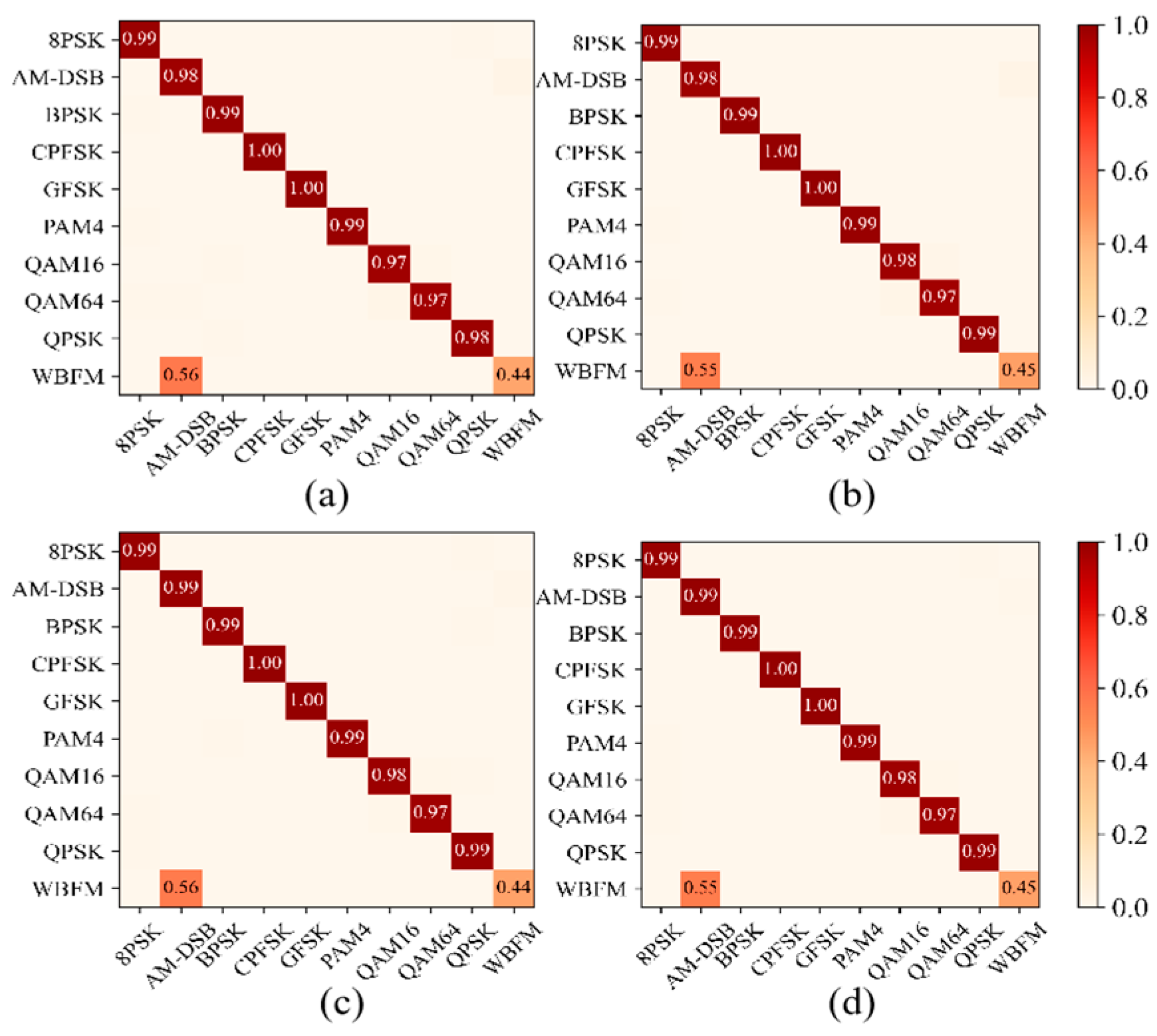
Figure 5 shows the confusion graph of ten modulation signals in 10 dB SNR with different correction methods. The performance of the correction module is better than that without it. However, these three correction methods only have slight differences because they only represent the predicted classification results and cannot directly reflect the specific recognition accuracy details.

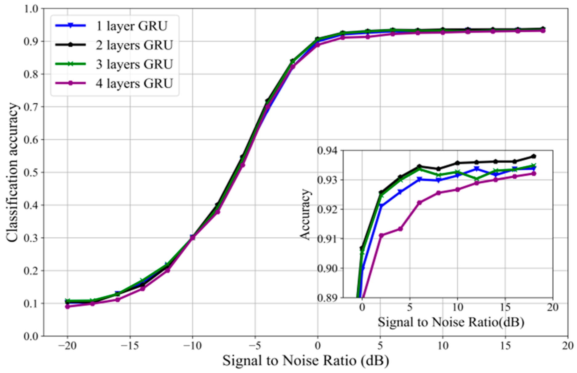
In the part before, an effective structure based on a two-layer GRU network was suggested; an experiment was then carried out to confirm it. First, set up a comparison experiment with different numbers of GRU layers: 1 layer, 2 layers, 3 layers, and 4 layers. Figure 6 indicates the performance of 2-layer GRU is better than the others. There is a little difference between the 3-layer GRU and 1-layer GRU in recognition accuracy, and 4-layer GRU is not as good as the other three groups due to overfitting.

Also, using the suggested two-layer GRU model, we confirmed the impact of the quantity of units in each layer and set up five groups of comparative experiments with 20, 30, 40, 50, and 60 different units, respectively. In this way, the most appropriate number of units to fit the neural network is determined. Figure 7 shows that the number of GRU units are 30 and 40 for the best performance, and the recognition accuracy is slightly better when the number of units is 40. The performance of other groups is poor due to insufficient training or too many learning features.

In a similar vein, the batch size has an impact on recognition accuracy. It shows how many samples were chosen for a training set. As a result, we conducted comparative studies to ascertain the neural network’s ideal batch size. Parallelizing stochastic gradient descent is challenging since it is continuous and employs small batches. When we divide the training instances among multiple working nodes, a bigger batch size enables us to calculate more in parallel. Model training can be greatly accelerated by doing this. Figure 8 demonstrates that the optimal performance is achieved when the batch size is 128. Large batches converge to sharp minimization, which varies substantially, while training with small batches tends to converge to flat minimization, which varies very minimally in the narrow neighborhood of minimization. Operational processing becomes slower than before when batch size increases, because batch size increases also result in a significant rise in time.

Through the previous experimental analysis, to determine the model parameters, we sought to assess the correlation between the iterative connection depicted in Figure 9 and the accuracy of the training loss value. As the number of iterations rose, the identification accuracy improved, and the function’s loss value steadily decreased, suggesting that the model’s convergence was adequate.

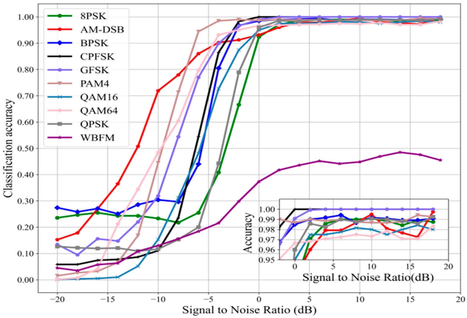
Figure 10 displayed the identification accuracy of 10 modulation signals under different SNRs. The maximum recognition accuracy was 93.79% when the SNR was at 18 dB. All signals except WBFM were properly detected, and the recognition accuracy was above 97% when the SNR was greater than 5 dB. The average recognition accuracy was higher than 90% when the SNR was greater than 0 dB. The difficulty is exacerbated by the fact that the WBFM signal in the dataset is produced by sampling analog audio sources, and there are silence cycles. The greatest recognition performance, the strongest anti-interference capacity against noise, and 100% accurate identification were all exhibited by GFSK and CPFSK. The outcome suggests that the technique may be applied for more accurate modulation recognition.

With 100% accurate identification, the greatest recognition performance, and the highest noise-cancelling capabilities, GFSK and CPFSK were the most effective. The results indicate that the method can be used for modulation recognition with higher accuracy.

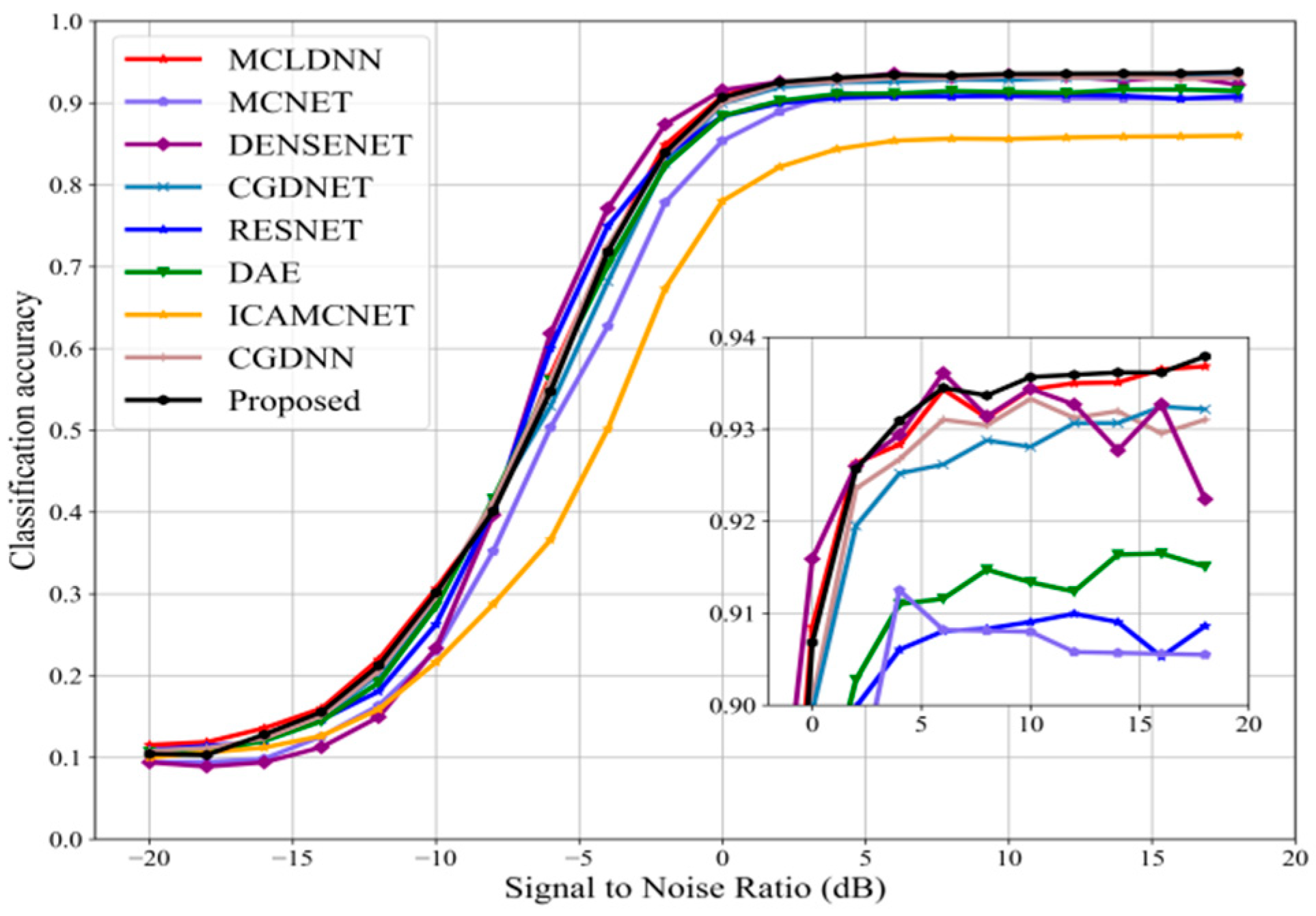
Furthermore, the network model presented in this research was sufficiently extended to be used for the problem of modulated signal identification. We conducted a comparison between the suggested strategy and eight popular network frameworks in order to determine its effectiveness. All of the aforementioned classifications made use of the RadioML2016.10b datasets and were balanced. The majority of the suggested method’s recognition accuracy rates display a leading level, as seen in Figure 11. The recognition accuracy rate has been consistently higher than 93% when SNR is higher than 5 dB. In comparison to other models, the DAE, RESNET, and MCNET models have poorer recognition accuracy. At 6 dB, DENSENET has the highest recognition rate of all the comparison models; however, at greater SNR, the recognition accuracy keeps decreasing. This is because the model has a lot of parameters, which leads to overfitting and lowers recognition accuracy. The model presented in this paper shows good performance at all signal-to-noise ratios.

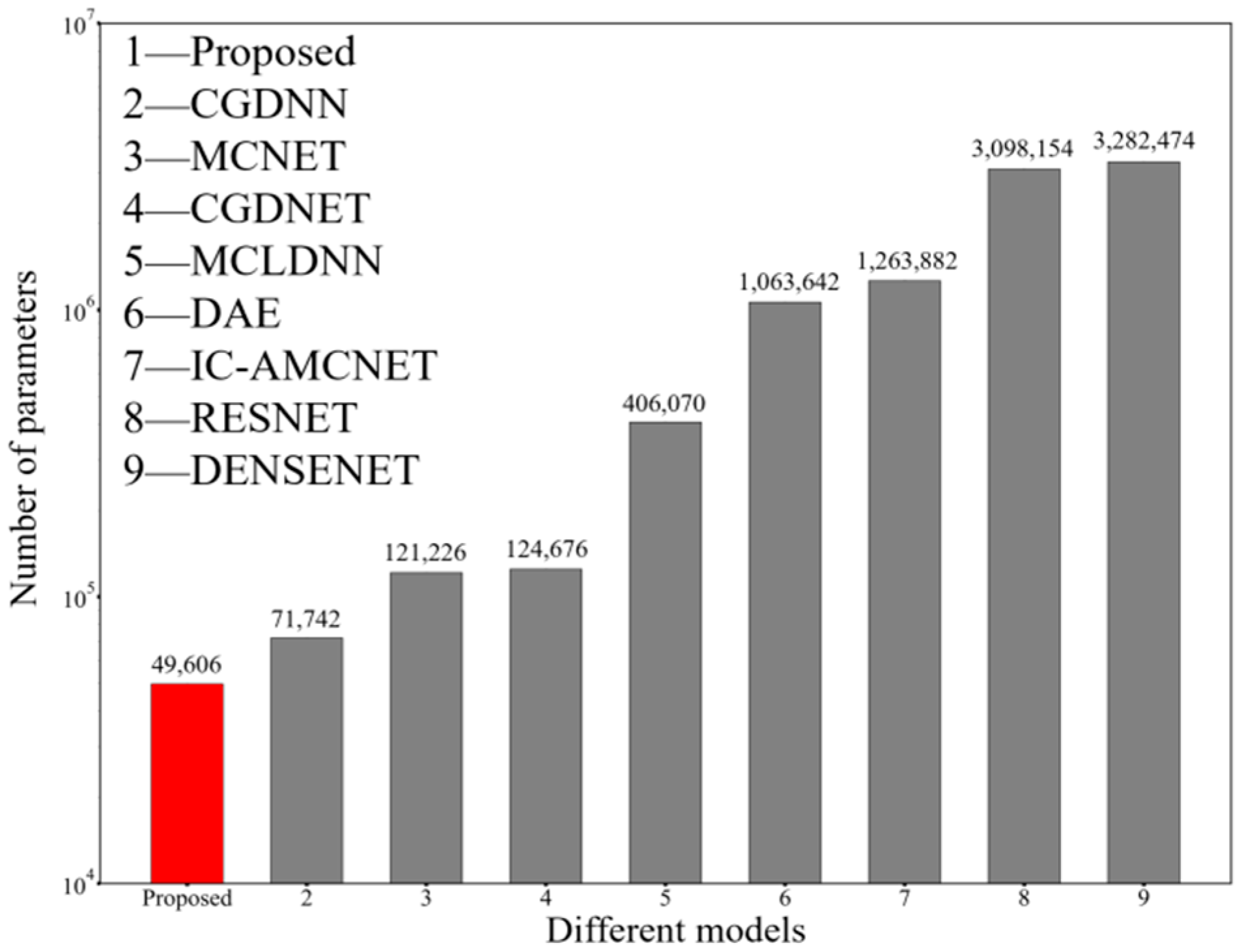
Similarly, as a lightweight index, Figure 12 shows that the proposed method uses the minimum parameter compared with the reported methods, and thus can decrease computational complexity 50% or more. This shows that the proposed method increases more training groups to improve high classification accuracy, and average recognition accuracy is also at a high level.

The detailed parameter comparison between the proposed model and the eight common signal modulation recognition network models shows that the parameter number of the proposed model is nearly 50% less than that of the CGDNN model with the least parameters, and nearly 98% less than that of the DENSNET model with the most parameters. This model has greater average and maximum accuracy than the other eight models that are currently in use. In order to attain the maximum recognition accuracy rate, the experiment expanded the number of training groups. Figure 10 shows that fewer groups are already able to attain the current acceptable recognition accuracy. The reduction of parameters can reduce training costs and improve training efficiency for future research. Other performance parameters are listed in

Table 2. Comprehensive comparison of performance evaluation of different models.

Model	Parameter	Training Time (s)	Training Epoch	Highest Accuracy	Average Accuracy
CGDNN [14]	71, 742	33	101	93.33	63.82
MCNET [16]	121,226	46	107	91.25	61.95
CGDNET [17]	124,676	40	157	93.24	63.34
MCLDNN [18]	406,070	90	69	93.68	63.78
DAE [19]	1,063,642	39	228	91.63	62.13
IC-AMCNET [20]	1,263,882	34	233	90.01	60.65
RESNET [21]	3,098,154	131	275	90.48	60.12
DENSENET [21]	3,282,474	189	298	93.27	63.67
Proposed	49,606	174	134	93.79	64.34

.

All experiments were conducted in the same experimental environment [22]. The MCNET, IC-AMCNET and DAE models do not use traditional RNN to extract time-domain feature of signals. CGDNET and MCLDNN use more convolutions to extract feature leads to need more convolution parameters. RESNET and DENSENET have complex parameters that require a huge training time. Our proposed scheme considers the impact of signal offset while maintaining minimal parameters and saving training resources.

4. Conclusions

In this paper, we focused on the time-domain characteristics of the signal and the offset effects on the signal. To save training resources and achieve the light weight of the model, we proposed a cascaded double-layer GRU network based on learnable correction modules, which can learn frequency and phase offset parameters. The double-layer GRU network can effectively use the time-domain characteristics of signals on the basis of minimal parameters. The results show that a reasonable tradeoff between the accuracy and the computational complexity can be achieved. The highest accuracy is up to 93.79% when SNR equals 18 dB, and the highest computational complexity has decreased by nearly 98%. The suggested approach offers a compelling technique for modulation identification.

We can keep reducing the model’s parameters in future work and investigate the connection between the recognition accuracy and the number of parameters that are explicitly lowered.