Game Theory-Based Interactive Control for Human–Machine Cooperative Driving

Abstract

To address the safety and efficient driving issues of human–machine shared control vehicles (HSCVs) in future complex traffic environments, this paper proposes a game theory-based interactive control method between HSCVs and surrounding autonomous vehicles (SVs) and involves considering different driving behaviors. In HSCV, a comprehensive driver model integrating steering control and speed control is designed based on the brain emotional learning circuit model (BELCM), and the control authority between the driver and the automation system is dynamically allocated through the evaluation of the driving safety field. Factors such as driving safety and travel efficiency that reflect personalized driving style are considered for modeling the uncertain behavior of SVs. In the interaction between HSCVs and SVs, a method based on game theory and distributed model predictive control (DMPC) that considers the uncertainty of SVs’ driving behavior is established and is finally integrated into a multi-objective constraint problem. The driver control input in an HSCV will also be introduced into the solution process. To demonstrate the feasibility of the proposed method, two test scenarios considering the driving characteristics of different SVs are established. The test results show that automation control systems can promptly stop the human driver’s dangerous operations in an HSCV and safely interact with multiple AVs with different driving characteristics.

1. Introduction

Benefiting from the advancement of science and technology, such as computer science, communication networks, and smart chips, autonomous driving technology has progressed rapidly in recent years. The Society of Automotive Engineers (SAE) used a six-level system (ranging from level 0 to level 5) in 2014 to define the degree of automation [1]. The current research on autonomous driving mainly focuses on the degree of level 3 [2], which allows for switching between fully autonomous and fully manual driving modes. However, a variety of unresolved issues need to be addressed before fully autonomous driving can be achieved, including ethical issues, laws and regulations, and technical bottlenecks [2,3,4,5]. In addition, keeping the driver out of the control loop for a long time will lead to driver over-reliance and situational awareness decline [4,6]. However, it is worth noting that automation control systems surpass humans in information storage, computing power, etc., while human drivers exceed automation in moral judgment and reasoning [2]. Shared control technology in intelligent driving can make full use of the strengths of human drivers and automation systems to compensate for each other’s weaknesses, which has been considered a transition to fully autonomous driving [7]. The concept of shared control was first proposed by Sheridan and Verplank in the field of industrial robots in 1978 [8]. Subsequent research developed it towards intelligent vehicles and derived the idea of a human–machine shared control vehicle (HSCV) [2,4,6].

The standard shared control system in an HSCV consists of a human driver, an automation control system, a control mechanism, and a controlled vehicle system [6]. The driver in a shared control system sits in the driving seat and controls the future movement of the vehicle by turning the steering wheel and adjusting the accelerator and brake pedals. The unique aspect of shared control in an HSCV is that the driver and the automation control system are simultaneously kept in the control loop to complete a specific driving task together [2]. The control mechanism is used to integrate the driver’s control commands and the control actions of the automation system and ultimately input them into the vehicle system. Based on the different control mechanisms, the shared control system in an HSCV can be divided into a haptic shared control system and an input mixing shared control system. The main difference between them is whether the control mechanism is mechanically coupled. Haptic shared control usually uses an electric power steering system to directly increase auxiliary torque to intervene and guide the driver’s control commands [9]. In contrast to haptic shared control, a steer-by-wire system can be used by an input mixing shared control system to allow the steering wheel to be mechanically decoupled from the road wheel. It then uses an intermediate controller to modify control commands entered by the driver before they are applied to the vehicle steering system [2].

Designing a proper control policy for the automation system is always one of the critical issues in the shared control system. An appropriate control policy is expected to consider drivers’ personalization and commands to minimize human–machine conflicts and guarantee driving safety and stability in changeable traffic scenarios [4,6]. For shared control, integrating driver modeling into the system to characterize driver behavior can increase mutual understanding between the driver and the automation system, thereby reducing human–machine conflicts [2,10]. Many studies based on driver models have been conducted, including the single-point preview model [2] and the two-point preview model [11,12], which are used to simulate the driver’s steering behavior in lane keeping scenarios and obstacle avoidance scenarios. Li et al. [13] adopted the idea in the work [14] that driver steering behavior can be simulated by model predictive control (MPC), and they designed a driver steering model based on MPC. A brain emotional learning circuit model (BELCM) was designed in [15] to simulate driver steering behavior, but it did not consider human–vehicle interaction. In terms of shared longitudinal control in an HSCV, the main contribution of this research direction focuses on using the haptic accelerator to perform vehicle following tasks [16,17]. In particular, the integrated control framework of driver steering control and speed control models in HSCVs requires more research.

For automation control systems, it is necessary to design shared controllers to assist drivers in driving safely and smoothly and to make timely interventions in dangerous situations. And there are a variety of shared controllers in HSCVs, which include a linear quadratic regulator (LQR) [18], Takagi–Sugeno (T-S) fuzzy control [11], ${\mathcal{H}}_{\inf }$ control [19], and MPC [20]. Compared with the above controller, MPC has the advantage of being suitable for solving multi-constraint and multi-variable optimization problems, and it has received widespread attention in the design of shared controllers for HSCVs [4,6,21]. In 2013 [22], Anderson et al. used constrained MPC to design a shared controller and then used a weighted summation method to integrate the control commands of the driver and the automation control system. However, this method ignored the adaptability of the shared controller to the driver’s control input. A novel shared controller is designed in [20,23], in which the driver’s control commands are integrated into the MPC’s cost function to form an optimization problem. Considering that the driver’s unreasonable operation will pose a safety threat to the vehicle, Liu et al. [24] added a driving control authority allocation strategy based on fuzzy logic in the shared controller. Another reference-free shared control framework based on MPC was designed by Huang et al. [25]. In this shared controller, constrained Delaunay triangles and collision time are used to determine the safe area, vehicle sideslip angle, and yaw angular rate, which are used to design stability constraints. Na et al. [26,27] use a non-cooperative MPC method to simulate the interaction between the driver and the controller, in which the driver steering controller and the automation controller need to minimize the cost function of cumulative trajectory errors while also considering the impact of their control outputs on each other. The above studies on shared controllers in HSCVs mainly focus on obstacle avoidance and lane keeping scenarios. However, previous research mentioned above on HSCV shared controllers focused primarily on static driving environments, such as safe avoidance of static obstacles on the road or lane keeping on a road without other vehicles, and it lacks consideration of the impact of complex factors such as vehicle interaction.

In the complex traffic environment of the future, it will be necessary for HSCVs to share the road with adjacent traffic participants. Some research on how to design a safe and effective control scheme for HSCVs to avoid SVs or static obstacles safely was conducted. In [20], a method was demonstrated that integrates driver control commands into a constrained MPC and defines an environmental envelope and a stable handling envelope in the shared controller to ensure safe and stable obstacle avoidance driving. In [28], the elliptical driving safety field is used to design a strategy to avoid surrounding vehicles for human–machine shared control. Yue et al. [29] developed a spatial collision risk system that allocates driving authority between the driver and the automation system to avoid surrounding vehicles. In [27], MPC and game theory are used to simulate the impact of the interaction between the driver and the automation system in obstacle avoidance scenarios. However, the status of obstacles or surrounding vehicles (SVs) is static or determined in the above studies while ignoring the influence of the behavioral changes of SVs. Advances in sensors and vehicle-to-vehicle communication technology have facilitated the development of connected autonomous vehicles (CAVs) [30]. The impact of the different driving styles (aggressive, normal, cautious) of vehicles on interactive behavior in lane changing and unsignalized roundabout scenarios has been studied in the field of CAVs [30,31,32]. However, current HSCV studies need to give more attention to complex traffic conditions, especially multi-vehicle interaction scenarios with different driving styles.

How to ensure safe driving between HSCVs and SVs in uncertain traffic environments, especially in multi-vehicle interaction scenarios with different driving styles, is still an open issue. Based on a non-cooperative game, this paper designs a safe, interactive control method for HSCVs with surrounding vehicles with different driving styles. The main contributions are as follows. (1) The driver’s control commands in the HSCV, as well as the uncertain driving behavior of SVs, especially the aggressive behavior of neighbor vehicles that suddenly change lanes or accelerate to occupy the road, are taken into account by the automation control system of the HSCV to ensure safe driving. (2) The coupling optimization problem of the HSCV in a multi-vehicle interaction scenario is transformed into a non-cooperative game obstacle avoidance control problem. The iterative optimal response method is adopted to find Nash equilibrium solutions for these non-cooperative games.

The structure of the article is as follows. Problem formulation and the overall system framework are described in Section 2. Section 3 displays the vehicle dynamics model and a comprehensive driver model considering lateral and longitudinal control. Then, Section 4 establishes the human–machine shared control model and shared control strategy and demonstrates the non-cooperative game interaction method between HSCV and SVs, considering different driving styles. In Section 5, the feasibility of the algorithm is tested and analyzed in different scenarios. Section 6 concludes this study.

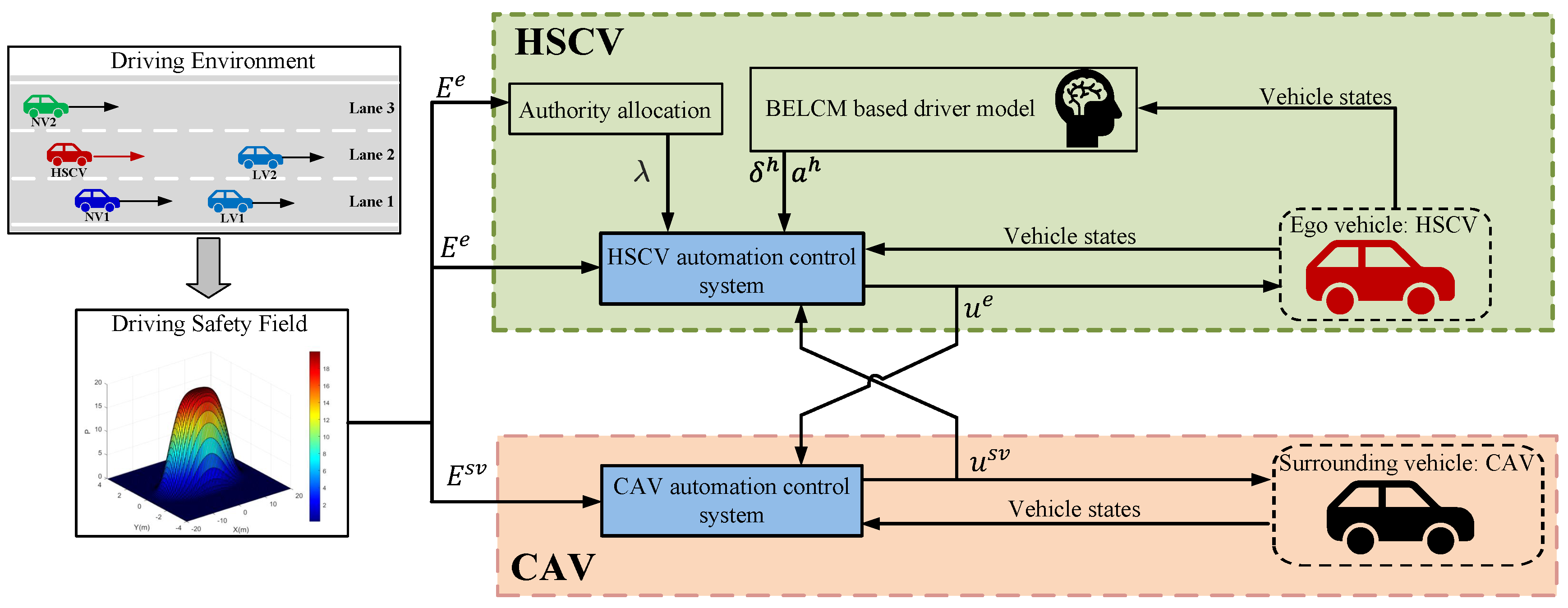
2. Problem Formulation

As introduced in Section 1, existing research on the traffic participants that HSCV needs to avoid in safe driving are usually set as static obstacles, or SVs, with fixed driving characteristics, and the motion state remains unchanged. However, there are significant differences in the driving styles of different drivers, and the research methods related to driving style recognition include the Markov model, K-means clustering, Bayesian learning, and other methods [31]. Usually, the three labels of aggressive, moderate, and cautious are used in many studies to distinguish driver styles [30,33,34,35]. Aggressive drivers often pursue traffic efficiency and perform sharp acceleration and steering behaviors. For example, an aggressive driver may suddenly accelerate and seize the road, preventing neighbor vehicles from changing lanes. Aggressive drivers even have the dangerous behavior of suddenly changing lanes and ignoring the existence of neighbor vehicles. However, cautious drivers worry about driving safety and will choose a lower speed and maintain a longer following distance. This article focuses on the impact of the dangerous behavior of SVs on HSCVs and how to safely control HSCVs rather than the classification of driving styles. The driving style of SVs will be designed based on the driving style cost function, in which two critical indicators of driving safety and travel efficiency that reflect personalized driving style will be taken into consideration.

Lane changing is a typical driving behavior of vehicles which is also prone to lead to traffic accidents, especially in high-speed scenarios. This paper mainly focuses on ensuring the safety control of an HSCV in the lane changing scenario, including the HSCV’s avoidance of the sudden lane changes of neighbor vehicles (NVs). The driving environment module in Figure 1 shows common driving scenarios in which the red vehicle driving on road 2 is an HSCV controlled by a human driver and an automation system. The vehicles on either side of the HSCV are represented as NV1 and NV2, respectively. The vehicles in front of the road are represented as leader vehicles (LVs). The HSCV is the subject of this study, and it can also be expressed as an ego vehicle, and all NVs and LVs around the HSCV can be called SVs. For the convenience of expression, superscript symbols e and $V_i$ are proposed to distinguish the HSCV from SVs, where i is the index of SVs.

The overall safety obstacle avoidance control framework of the HSCV is illustrated in Figure 1. Firstly, before the HSCV executes vehicle control commands, its automation control system needs to integrate the control commands of the driver and the control system based on the allocated driving authority. The driver’s control commands are simulated by the brain emotional learning circuit model (BELCM), and the driving control authority between the driver and the control system is dynamically adjusted in real time by the driving safety field simulated by the driving environment information. In addition to the driver control input, the HSCV automation control system must also consider the interaction with SVs with different driving styles, which the driving style cost function will simulate. Finally, the non-cooperative game method was adopted to find the optimal solution for the HSCV to achieve safe control and obstacle avoidance.

3. Driver and Vehicle Models

Inspired by the emotional learning ability of the human cerebral cortex, Balkenius and Moren proposed a BELCM that can reflect the human-like control mechanism [36]. Many studies have proven that it has the advantages of good robustness, low computational complexity, and good real-time performance [15], which makes it widely used, such as in motor control [37], speech emotion recognition [38], and lateral control of CAVs [15]. However, driver models that integrate lateral and longitudinal control require more research.

A comprehensive driver model considering the driver’s lateral and longitudinal control is established in this section. First, the working principle of the BELCM is illustrated. Its block diagram is shown in Figure 2. The details of the established driver model based on the BELCM algorithm are explained, and finally, the vehicle dynamics model is introduced.

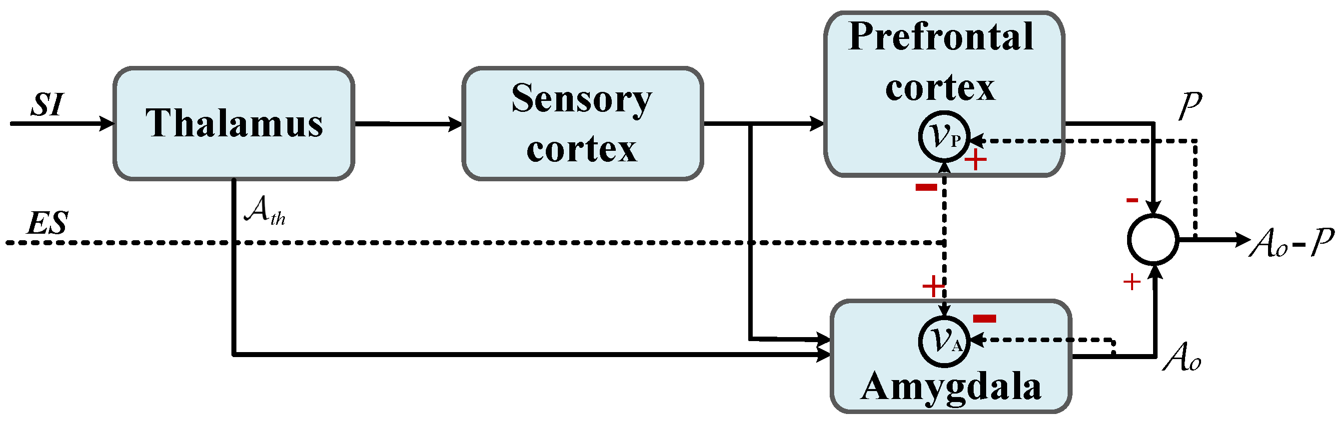
3.1. Brain Emotional Learning Circuit Model

The BELCM simulates the working mechanism of the brain’s emotional learning process. The final output signal of the BELCM is expressed as the amygdala output signal ${\mathcal{A}}_o$ minus the correction signal $\mathcal{P}$ output by the prefrontal cortex. This model requires a hint of emotional signal (ES) and external stimulus input (SI) to assist in the learning process. First, the thalamus receives the external SI and transmits its maximum value ${\mathcal{A}}_{th}$ to the amygdala.

$${\mathcal{A}}_{th}=max\left(SI\right),SI={\left[I_1,I_2,\cdots ,I_i\right]}^T,i=1,2,\cdots ,n$$

(1)

Other $SI$s will be output by the thalamus to the sensory cortex for processing, and then the sensory cortex will pass them to the amygdala and prefrontal cortex. The amygdala’s signal processing will be explained first. Each input signal $I_i$ corresponds to a node with a dynamic coefficient ${\mathcal{V}}_{A_i}$ in the amygdala, and the amygdala output signal ${\mathcal{A}}_o$ is obtained after weighted summation. In addition, the learning rate ${\alpha }_1$ and $\Delta {\mathcal{V}}_{A_i}$ will be used to dynamically adjust ${\mathcal{V}}_{A_i}$, where $\Delta {\mathcal{V}}_{A_i}$ is updated by the error between ${\mathcal{A}}_o$ and $ES$, ${\alpha }_1\in (0,1)$. The mathematical model of the amygdala can be written as follows:

$$\left\{\begin{array}{c}{\mathcal{A}}_o={\mathcal{A}}_{th}+\sum _{i=1}^n{I}_i{\mathcal{V}}_{A_i}\hfill \\ \Delta {\mathcal{V}}_{A_i}={\alpha }_1·I_i·max\left(0,ES-{\mathcal{A}}_{th}-\sum _{i=1}^n{I}_i{\mathcal{V}}_{A_i}\right)\hfill \end{array}\right.$$

(2)

The prefrontal cortex’s process of generating the correction signal $\mathcal{P}$ is similar to the working principle of the amygdala. There are nodes in the prefrontal cortex corresponding to the input signal $I_i$, and the dynamic weight coefficient of each node is adjusted according to the learning rate ${\alpha }_2$ and $\Delta {\mathcal{V}}_{P_i}$, ${\alpha }_2\in (0,1)$. Its working mechanism is defined as follows:

$$\left\{\begin{array}{c}\mathcal{P}=\sum _{i=1}^n{I}_i{\mathcal{V}}_{P_i}\hfill \\ \Delta {\mathcal{V}}_{P_i}={\alpha }_2·I_i·\left(\sum _{i=1}^n{I}_i{\mathcal{V}}_{A_i}-\mathcal{P}-ES\right)\hfill \end{array}\right.$$

(3)

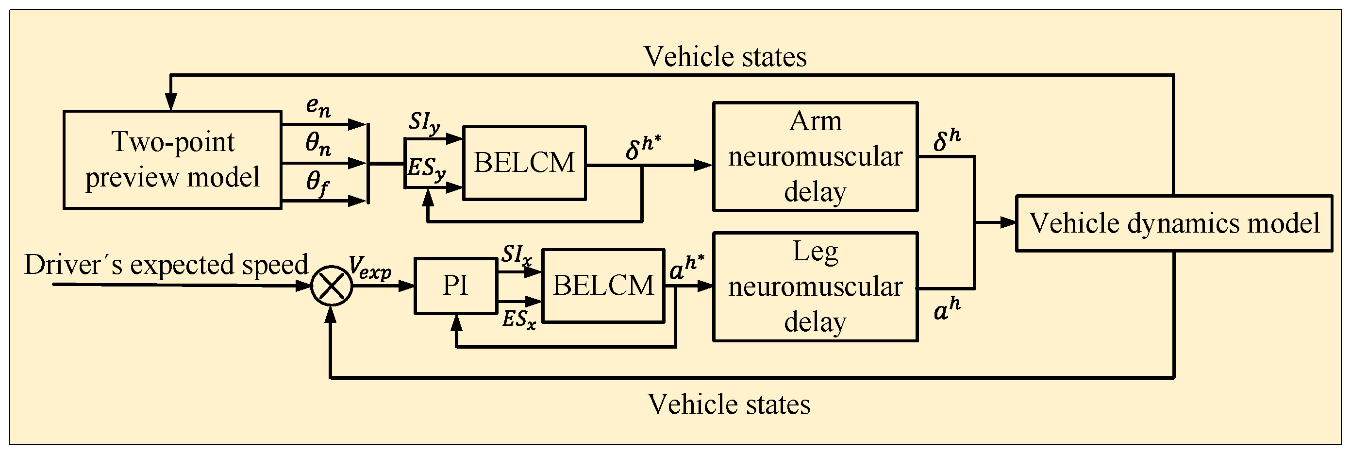
3.2. BELCM-Based Driver Model

This section introduces the driver steering model and longitudinal control model in sequence. It should be noted that the subscripts y and x will be used to distinguish their parameters. The driver model’s overall block diagram and workflow are shown in Figure 3 and Algorithm 1, respectively.

Algorithm 1 Workflow of driver model based on BELCM

1: Parameter initialization: ${\gamma }_y,{ϵ}_y,{\alpha }_1,{\gamma }_x,{ϵ}_x,{\alpha }_2$ 2: Set initial value to 0: ${\mathcal{V}}_{A_y},{\mathcal{V}}_{P_y},{\mathcal{V}}_{A_x},{\mathcal{V}}_{P_x}$ 3: Input: $e_n,{\theta }_n,{\dot{\theta }}_f,e_v$ 4: Calculate: $S{I}_y,E{S}_y,S{I}_x,E{S}_x$ 5: Calculate: $\Delta {\mathcal{V}}_{A_y},\Delta {\mathcal{V}}_{P_y},\Delta {\mathcal{V}}_{A_x},\Delta {\mathcal{V}}_{P_x}$ 6: Update: ${\mathcal{V}}_{A_y},{\mathcal{V}}_{P_y},{\mathcal{V}}_{A_x},{\mathcal{V}}_{P_x}$ 7: Output: ${\delta }^{h^{\ast }},a^{h^{\ast }}$, ${\delta }^h,a^h$ 8: Repeat: steps 3–7

3.2.1. Driver Steering Control Model

Studies have shown that the driver’s steering behavior is guided by observing a near point with the preview angle ${\theta }_n$ and a far point with the preview angle ${\theta }_f$ on the road, which can be represented by the two-point preview model [11]. For the detailed derivation process, one can refer to [12]. In this paper, $e_n,{\theta }_n$, and ${\theta }_f$ are adopted as the external stimulus signals $S{I}_y$ received by the thalamus for lateral control, where $e_n$ represents the lateral error at the near point. $E{S}_y$, involved in vehicle steering control in the brain’s emotional learning circuit, can be formed through long-term learning. $S{I}_y$ and $E{S}_y$ are defined as follows:

$$\left\{\begin{array}{c}S{I}_y={\left[{\gamma }_{y_1}{e}_n,{\gamma }_{y_2}{\theta }_n,{\gamma }_{y_3}{\dot{\theta }}_f\right]}^T\hfill \\ E{S}_y={ϵ}_{y_1}{e}_n+{ϵ}_{y_2}{\theta }_n+{ϵ}_{y_3}{\dot{\theta }}_f+{ϵ}_{y_4}{\delta }^h\hfill \end{array}\right.$$

(4)

where ${ϵ}_{y1}\sim {ϵ}_{y4}$ and ${\gamma }_{y1}\sim {\gamma }_{y3}$ are the weighted coefficients of $E{S}_y$ and the weighted coefficients of $S{I}_y$, respectively. The weight coefficients in the amygdala and prefrontal cortex can be expressed as matrices ${\mathcal{V}}_{A_y}=\left[{\mathcal{V}}_{A_{y1}},{\mathcal{V}}_{A_{y2}},{\mathcal{V}}_{A_{y3}},{\mathcal{V}}_{A_{th}}\right]$ and ${\mathcal{V}}_{P_y}=\left[{\mathcal{V}}_{P_{y1}},{\mathcal{V}}_{P_{y2}},{\mathcal{V}}_{P_{y3}}\right]$, respectively. Finally, the ideal output of steering control signals in the BELCM is as follows:

$${\delta }^{h^{\ast }}={\mathcal{V}}_{A_y}\left[\begin{array}{c}S{I}_y\hfill \\ A_{th}\hfill \end{array}\right]-{\mathcal{V}}_{P_y}S{I}_y$$

(5)

However, there is a time delay before the arm muscles execute the steering signal transmitted by the driver’s brain, and this delay characteristic can be simulated by the arm neuromuscular system (NMS) [26]. The state space equation of the NMS is as follows:

$$\begin{array}{cc}\hfill \left\{\begin{array}{c}{\dot{\delta }}_{\mathrm{nms}}^h\hfill \\ {\ddot{\delta }}_{\mathrm{nms}}^h\hfill \end{array}\right\}& =\left[\begin{array}{cc}0& 1\\ -{\omega }_n^2& -2\xi {\omega }_n\end{array}\right]\left\{\begin{array}{c}{\delta }_{\mathrm{nms}}^h\hfill \\ {\dot{\delta }}_{\mathrm{nms}}^h\hfill \end{array}\right\}+\left[\begin{array}{c}0\\ {\omega }_n^2\end{array}\right]{\delta }^{h^{\ast }}\hfill \\ \hfill {\delta }^h& =\left[\begin{array}{cc}1\hfill & 0\hfill \end{array}\right]\left\{\begin{array}{c}{\delta }_{\mathrm{nms}}^h\\ {\dot{\delta }}_{\mathrm{nms}}^h\end{array}\right\},\hfill \end{array}$$

(6)

where ${\omega }_n$ and $\xi$ represent the NMS’s natural frequency and damping ratio, respectively.

3.2.2. Driver Longitudinal Control Model

The driver’s longitudinal control of the vehicle can be simulated by the BELCM. The deviation $e_v$ between the vehicle’s longitudinal speed and the driver’s desired speed and the accumulation of $e_v$ are used as the stimulus signals $S{I}_x$ for longitudinal control. Similar to the driver steering control model, the longitudinal hint of the emotional signal $E{S}_x$ will be formed in the driver’s mind. The definitions of $S{I}_x$ and $E{S}_x$ are defined as follows:

$$\left\{\begin{array}{c}S{I}_x={\left[{\gamma }_{x_1}{e}_v,{\gamma }_{x_2}\int e_v\mathrm{d}t\right]}^T\hfill \\ E{S}_x={ϵ}_{x_1}{e}_v+{ϵ}_{x_2}\int e_v\mathrm{d}t+{ϵ}_{x_3}{a}^h\hfill \end{array}\right.$$

(7)

where ${ϵ}_{x1}\sim {ϵ}_{x3}$ and ${\gamma }_{x1}\sim {\gamma }_{x2}$ are the weighted coefficients of $E{S}_x$ in the amygdala and the weighted coefficients of $S{I}_x$, respectively. There is a delay when the driver executes the acceleration command transmitted from the brain. This delay characteristic can be approximated by the first-order lead-lag element. Finally, the BELCM outputs the driver’s ideal acceleration control as follows:

$$a^{h^{\ast }}={\mathcal{V}}_{A_x}\left[\begin{array}{c}S{I}_x\\ A_{th}\end{array}\right]-{\mathcal{V}}_{P_x}S{I}_x$$

(8)

$$a^h=\frac{e^{-{\tau }_{d1}s}}{1+{\tau }_{d2}s}{a}^{h^{\ast }}$$

(9)

where ${\tau }_{d1}$ and ${\tau }_{d2}$ are two delay parameters related to the driver’s brain signal processing and muscle working process and s represents the Laplacian.

3.3. Vehicle Model

In this paper, we adopt a three-degrees-of-freedom vehicle dynamics model [25], and its differential equation can be expressed as follows:

$$\left\{\begin{array}{c}{\dot{v}}_y=-v_x\omega +\frac{1}{m}\left(F_{yf}+F_{yr}\right)\hfill \\ {\dot{v}}_x=v_y\omega +a\hfill \\ \dot{\omega }=\frac{1}{J_z}\left(l_a{F}_{yf}-l_b{F}_{yr}\right)\hfill \\ \dot{Y}=v_{x}sin\varphi +v_{y}cos\varphi \hfill \\ \dot{X}=v_{x}cos\varphi -v_{y}sin\varphi \hfill \end{array}\right.$$

(10)

where X and Y are the longitudinal and lateral displacements of the vehicle, respectively. $v_x$, $v_y$, $\varphi$, and $\omega$ represent the vehicle’s longitudinal speed, lateral speed, heading angle, and yaw rate. a represents the acceleration of the vehicle. m and $J_z$ denote vehicle mass and moment of inertia. $l_a$ and $l_b$ represent the distances from the front and rear axles to the center of mass, respectively. Assuming that the tires work in the linear region, the lateral tire forces of the front and rear wheels can be approximately expressed as $F_{yf}\simeq -2C_f\left(\frac{v_y+l_a\omega }{v_x}-{\delta }_f\right)$ and $F_{yr}\simeq -2C_r\left(\frac{v_y-l_b\omega }{v_x}\right)$, respectively, where $C_f$ and $C_r$ indicate the stiffness coefficients of the front and rear tires, respectively.

4. Vehicle Interactive Control Strategy

The HSCV obstacle avoidance safety control method based on game theory is demonstrated in this section. First, the method of shared control between the driver and the automation system based on the driving risk field in the HSCV is introduced. Then, the human–machine shared control model and motion prediction are explained. Next, the design of the driving style cost function of surrounding vehicles is explained. Finally, the method of the HSCV interacting with surrounding vehicles is demonstrated.

4.1. Shared Control Strategy

This section will introduce methods for integrating driver and automation system control inputs and strategies for driving control authority allocation. First, we present the driving risk field, which is used to design rules that dynamically regulate the authority allocation between the automation system and the driver. The driving safety field E generates a potential field through the potential field function [39,40]. Then, we explain how the control inputs of these two agents are dynamically integrated.

4.1.1. Driving Safety Field

The driving safety field E is an effective method to dynamically assess the degree of driving risk in the ego vehicle through the surrounding environment. It mainly consists of the road potential field, the obstacle potential field, and the driver behavior field [28]. In this paper, an obstacle potential field $E_o$ is adopted to construct the driving safety field.

The obstacle potential field is used to assess the impact of obstacles on the road that pose a risk of collision with objective vehicles. It mainly includes surrounding vehicles moving on the road, stationary obstacles, or stopped vehicles. Our study only considers the obstacle potential field between the objective vehicle and surrounding moving vehicles. The objective vehicle can be either an HSCV or CAV on the road, and its potential field value under the coordinate $(X,Y)$ is defined as follows [31]:

$$\left\{\begin{array}{cc}\hfill & E^{V_i}(X,Y)=k^{obs}·e^{-{\left\{\frac{{\left(X-X^{V_i}\right)}^2}{2·{\sigma }_x^2}+\frac{{\left(Y-Y^{V_i}\right)}^2}{2·{\sigma }_y^2}\right\}}^{c_1}+c_2{v}_x^{V_i}\xi }\hfill \\ \hfill & \begin{array}{c}\xi =sgn(X-X^{V_i})\frac{{\left(X-X^{V_i}\right)}^2}{2{\sigma }_x^2}/\sqrt{\frac{{\left(X-X^{V_i}\right)}^2}{2{\sigma }_x^2}+\frac{{\left(Y-Y^{V_i}\right)}^2}{2{\sigma }_y^2}}\end{array}\hfill \end{array}\right.$$

(11)

$(X^{V_i},Y^{V_i})$ is the position of the center of mass of $V_i$ with respect to the objective vehicle, where the surrounding vehicle consists of the LV and NV around the objective vehicle. The convergence coefficients ${\sigma }_x$ and ${\sigma }_y$ are used to adjust the influence range of the longitudinal and lateral obstacle potential fields, respectively. $v_x^{V_i}$ is the longitudinal velocity of the moving obstacle vehicle. $k^{obs}$, $c_1$, and $c_2$ represent the shape coefficients.

4.1.2. Strategies for Authority Allocation

Reasonable control authority allocation strategy design between the driver and the automation control system is significant for HSCVs. The purpose of designing this control authority allocation strategy in our study is to dynamically adjust the driving authority between the driver and the automation control system for safety control. Considering that vehicle speed and driving risk fields pose major threats to drivers and vehicles in the traffic environment, the dynamic authority allocation strategy is designed based on the driving safety field described in Section 4.1.1 and the driving speed of the ego vehicle.

The normalized value of the driving safety field E is P, and its critical value is set to approximately 0.5. Initially, as its value continues to increase from 0, the driver’s driving authority will continue to decrease, and more driving authority will be allocated to the automation system to assist the driver in safe driving. Considering that changes in driving authority will cause the driver to be alert to the surrounding environment and make relevant driving responses, when the value of E exceeds about 0.5, the system will gradually release more driving authority to the driver for safe control. Figure 4 shows the curve graph of the designed driving authority allocation strategy. The formula for control authority allocation is defined as follows [41]:

$$\lambda \left(k\right)=1-{\sigma }_1{\left(E\left(k\right)\right)}^{{\sigma }_2-{\sigma }_5{V}^e\left(k\right)}·e^{\left(\frac{{\sigma }_3+{\sigma }_5{V}^e\left(k\right)}{E\left(k\right)-{\sigma }_4}\right)}$$

(12)

${\sigma }_1\sim {\sigma }_5$ is an adjustable coefficient greater than 0. $E\left(k\right)$ and $V^e\left(k\right)$ are the normalized driving safety field value and HSCV longitudinal speed at time k.

4.1.3. Human–Machine Shared Control Model

In an HSCV, driver and automation system control inputs are integrated to control the vehicle jointly. The continuous state equation of the vehicle–driver model is as follows:

$$\dot{\mathbf{x}}\left(t\right)={\mathbf{A}}_c\mathbf{x}\left(t\right)+\lambda {\mathbf{B}}_c{\mathbf{u}}^h\left(t\right)+(1-\lambda ){\mathbf{B}}_c{\mathbf{u}}^e\left(t\right)$$

(13)

The subscripts h and e are used to distinguish human driver control inputs and automation system control inputs, respectively, as well as their associated matrices. Where the vehicle status vector is $\mathbf{x}={\left[\begin{array}{cccccc}{v}_y\hfill & v_x\hfill & \varphi \hfill & \omega \hfill & Y\hfill & X\hfill \end{array}\right]}^{\mathrm{T}}$, control input vectors are ${\mathbf{u}}^e=$${\left[\begin{array}{cc}{\delta }^e\hfill & a^e\hfill \end{array}\right]}^T$ and ${\mathbf{u}}^h=$${\left[\begin{array}{cc}{\delta }^h\hfill & a^h\hfill \end{array}\right]}^T$. The matrices ${\mathbf{A}}_c$ and ${\mathbf{B}}_c$ are defined as follows.

$$\begin{array}{cc}\hfill {\mathbf{A}}_c& =\left[\begin{array}{cccccc}-\frac{2C_f+2C_r}{m{v}_x}& 0& 0& -v_x+\frac{2C_r{l}_b-2C_f{l}_a}{m{v}_x}& 0& 0\\ \omega & 0& 0& 0& 0& 0\\ 0& 0& 0& 1& 0& 0\\ -\frac{2C_f{l}_a-2C_r{l}_b}{J_z{v}_x}& 0& 0& -\frac{2C_f{l}_a^2+2C_r{l}_b^2}{J_z{v}_x}& 0& 0\\ 1& 0& v_x& 0& 0& 0\\ 0& 1& -v_y& 0& 0& 0\end{array}\right]\hfill \\ \hfill {\mathbf{B}}_c& ={\left[\begin{array}{cccccc}\frac{2C_f}{m}& 0& 0& \frac{2C_f{l}_a}{J_z}& 0& 0\\ 0& 1& 0& 0& 0& 0\end{array}\right]}^{\mathrm{T}}\hfill \end{array}$$

In computer programs, it is necessary to use the sampling time $T_s$ to discretize the continuous form of the formula. The discrete state equation can be obtained as follows:

$$\begin{array}{cc}\hfill \mathbf{x}(k+1)& =\mathbf{A}\mathbf{x}\left(k\right)+\lambda \mathbf{B}{\mathbf{u}}^h\left(k\right)+(1-\lambda )\mathbf{B}{\mathbf{u}}^e\left(k\right)\hfill \end{array}$$

(14a)

$$\begin{array}{cc}\hfill \mathbf{z}\left(k\right)& =\mathbf{C}\mathbf{x}\left(k\right)\hfill \end{array}$$

(14b)

where k represents the discrete time index and the matrix discretization method is $\mathbf{A}={\mathbf{I}}_6+T_s\ast {\mathbf{A}}_c,\mathbf{B}=T_s\ast {\mathbf{B}}_c$. $\mathbf{z}$ is a matrix that filters $\mathbf{x}$ according to the control target, and $\mathbf{C}=\left[\begin{array}{cccccc}0\hfill & 0\hfill & 1\hfill & 0\hfill & 0\hfill & 0\hfill \\ 0\hfill & 0\hfill & 0\hfill & 0\hfill & 1\hfill & 0\hfill \end{array}\right]$ is the slack matrix, used for the selection of vehicle state.

4.2. Motion Prediction for HSCVs

The future states of HSCVs and SVs are related to their current states and control inputs. In an HSCV, the automation system can obtain driver control commands $u^h$ through sensors, and it will use the MPC controller to compensate for the driver’s behavior based on the allocated driving authority $\lambda$ and surrounding environment information. Assuming that the prediction time domain and the control time domain are $N_p$ and $N_c$, respectively, the prediction Equation (14) is rewritten as follows:

$$\mathbf{Z}\left(k\right)=\mathsf{\Psi }\mathbf{x}\left(k\right)+\lambda {\mathsf{\Theta }}_1{\mathbf{U}}^h\left(k\right)+(1-\lambda ){\mathsf{\Theta }}_2{\mathbf{U}}^e\left(k\right)$$

(15)

It is worth noting that the prediction output of an HSCV without driver participation in driving control is similar to that of SVs, and its degradation form is as follows:

$$\mathbf{Z}\left(k\right)=\mathsf{\Psi }\mathbf{x}\left(k\right)+{\mathsf{\Theta }}_2{\mathbf{U}}^e\left(k\right)$$

(16)

The expansion of the above formula is as follows:

$$\begin{array}{cc}\hfill & \mathbf{Z}\left(k\right)=\left\{\begin{array}{c}\mathbf{z}(k+1)\\ \mathbf{z}(k+2)\\ ⋮\\ \mathbf{z}\left(k+N_u\right)\\ ⋮\\ \mathbf{z}\left(k+N_p\right)\end{array}\right\},\mathsf{\Psi }=\left[\begin{array}{c}\mathbf{C}\mathbf{A}\\ \mathbf{C}{\mathbf{A}}^2\\ ⋮\\ \mathbf{C}{\mathbf{A}}^{N_u}\\ ⋮\\ \mathbf{C}{\mathbf{A}}^{N_p}\end{array}\right],{\mathsf{\Theta }}_{\mathbf{2}}=\left[\begin{array}{cccc}\mathbf{C}\mathbf{B}& 0& \cdots & 0\\ \mathbf{C}\mathbf{A}\mathbf{B}& \mathbf{C}\mathbf{B}& \cdots & 0\\ \cdots & \cdots & \cdots & \ddots \\ \mathbf{C}{\mathbf{A}}^{N_c-1}\mathbf{B}& \mathbf{C}{\mathbf{A}}^{N_c-2}\mathbf{B}& \cdots & \mathbf{C}{\mathbf{A}}^0\mathbf{B}\\ \cdots & \cdots & \cdots & \ddots \\ \mathbf{C}{\mathbf{A}}^{N_p-1}\mathbf{B}& \mathbf{C}{\mathbf{A}}^{N_p-2}\mathbf{B}& \cdots & \mathbf{C}{\mathbf{A}}^{N_p-N_c}\mathbf{B}\end{array}\right]\hfill \\ \hfill & {\mathbf{U}}^h\left(k\right)=\left\{\begin{array}{c}{\mathbf{u}}^h\left(k\right)\\ {\mathbf{u}}^h(k+1)\\ {\mathbf{u}}^h(k+2)\\ ⋮\\ {\mathbf{u}}^h\left(k+N_u-2\right)\\ {\mathbf{u}}^h\left(k+N_u-1\right)\end{array}\right\},{\mathbf{U}}^e\left(k\right)=\left\{\begin{array}{c}{\mathbf{u}}^e\left(k\right)\\ {\mathbf{u}}^e(k+1)\\ {\mathbf{u}}^e(k+2)\\ ⋮\\ {\mathbf{u}}^e\left(k+N_u-2\right)\\ {\mathbf{u}}^e\left(k+N_u-1\right)\end{array}\right\},{\mathsf{\Theta }}_1\left(k\right)=\left[\begin{array}{c}\mathbf{C}\mathbf{B}\\ \mathbf{C}\mathbf{B}+\mathbf{C}\mathbf{A}\mathbf{B}\\ ⋮\\ \sum _{i=0}^{N_p-1}\mathbf{C}{\mathbf{A}}^i\mathbf{B}\end{array}\right]\hfill \end{array}$$

(17)

The MPC controller in an HSCV will consider the control sequence amplitude and track the reference target to match the driver’s operation command. At the same time, the driver’s steering control and speed control commands are assumed to remain unchanged in the prediction time domain. Its cost function is defined as follows:

$$\begin{array}{cc}\hfill \underset{\mathbf{u}}{min}J\left(k\right)=& {\left[\mathbf{Z}\left(k\right)-{\mathbf{Z}}_{ref}\left(k\right)\right]}^{\mathrm{T}}\mathbf{Q}\left[\mathbf{Z}\left(k\right)-{\mathbf{Z}}_{ref}\left(k\right)\right]+{\mathbf{U}}^e{\left(k\right)}^{\mathrm{T}}\mathbf{R}{\mathbf{U}}^e\left(k\right)\hfill \end{array}$$

(18a)

$$\begin{array}{cc}\hfill \mathrm{s}.\mathrm{t}.& \mathbf{x}(k+1)=\mathbf{A}\mathbf{x}\left(k\right)+\lambda \mathbf{B}{\mathbf{u}}^h\left(k\right)+(1-\lambda )\mathbf{B}{\mathbf{u}}^e\left(k\right)\hfill \end{array}$$

(18b)

$$\begin{array}{cc}\hfill & \mathbf{z}\left(k\right)=\mathbf{C}\mathbf{x}\left(k\right)\hfill \end{array}$$

(18c)

$$\begin{array}{cc}\hfill & \left[\begin{array}{c}-{\delta }_{lim}^e\\ -a_{lim}^e\end{array}\right]⩽{\mathbf{u}}^e\left(k\right)⩽\left[\begin{array}{c}{\delta }_{lim}^e\\ a_{lim}^e\end{array}\right]\hfill \end{array}$$

(18d)

$$\begin{array}{cc}\hfill & \left[\begin{array}{c}-\Delta {\delta }_{lim}^e\\ -\Delta a_{lim}^e\end{array}\right]⩽\Delta {\mathbf{u}}^e\left(k\right)⩽\left[\begin{array}{c}\Delta {\delta }_{lim}^e\\ \Delta a_{lim}^e\end{array}\right]\hfill \end{array}$$

(18e)

where $\mathbf{Q}$ and $\mathbf{R}$ are the output weight matrix and the control input weight matrix, respectively. ${\mathbf{Z}}_{ref}$ is the target state matrix related to the reference trajectory, which consists of the reference heading angle ${\varphi }_{ref}$ and the reference lateral position $Y_{ref}$. The maximum amplitude and maximum change rate of the vehicle’s front wheel angle are represented by ${\delta }_{lim}^e$ and $\Delta {\delta }_{lim}^e$, respectively. $a_{lim}^e$ and $\Delta a_{lim}^e$ are used to set the upper and lower bounds of vehicle acceleration and limit the change rate of acceleration, respectively.

After solving the above constrained optimization problem, the optimal control sequence ${{\mathbf{U}}^e}^{\ast }\left(k\right)$ can be obtained as follows:

$${{\mathbf{U}}^e}^{\ast }\left(k\right)={\left[{{\mathbf{u}}^e}^{\ast }\left(k\right),{{\mathbf{u}}^e}^{\ast }(k+1),\cdots ,{{\mathbf{u}}^e}^{\ast }\left(k+N_c-1\right)\right]}^T$$

(19)

The first element in ${{\mathbf{U}}^e}^{\ast }\left(k\right)$ will be selected to control the movement of the vehicle, thus assisting the driver in driving the vehicle. In terms of driverless vehicles, many related motion prediction methods have been developed, which can be referred to in [31].

4.3. Driving Cost Function

Surrounding vehicles with different driving styles will cause different trade-offs between driving safety and travel efficiency. This section presents the design method of simulating SVs’ driving styles and the design of the safety cost function in an HSCV.

4.3.1. Driving Style Cost Function of SVs

This article considers two important indicators reflecting the personalized driving styles of surrounding vehicles: driving safety and travel efficiency. The driving style cost function of surrounding vehicles $V_i$ is expressed as follows:

$$J^{V_i}=(1-k^{V_i})J_s^{V_i}+k^{V_i}{J}_e^{V_i}$$

(20)

where $J_s^{V_i}$, $J_e^{V_i}$ represent the cost functions of driving safety and travel efficiency. It is worth noting that $k^{V_i}$ is a weight coefficient used to adjust the degree of aggressiveness of driving style, $k^{V_i}\in (0,1)$. The larger value of $k^{V_i}$ represents a driving style that pursues higher travel efficiency and lower driving safety, which means a higher level of aggressiveness. On the contrary, the smaller the value of $k^{V_i}$, the lower the level of aggressiveness. The corresponding relationship between the weight coefficient and the driving aggressiveness level is defined in

Table 1. Weight coefficient of driving style cost function.

Level of Aggressiveness	High Level	Moderate Level	Low Level
Coefficient: $k^{V_i}$	0.9	0.5	0.1

.

The cost function of driving safety $J_s^{Vi}$ consists of three parts, namely, vehicle longitudinal threat, lateral threat, and lane change threat. It is defined as follows:

$$J_s^{V_i}=J_{s-x}^{V_i}+J_{s-y}^{V_i}+J_{s-lc}^{V_i}$$

(21)

where $J_{s-x}^{V_i}$, $J_{s-y}^{V_i}$, $J_{s-lc}^{V_i}$, respectively, denote the longitudinal, lateral, and lane change threats in the surrounding environment of vehicle $V_i$.

In terms of longitudinal threat $J_{s-x}^{V_i}$, the relative longitudinal speed and distance between vehicle $V_i$ and LV are used to design its cost function.

$$\begin{array}{cc}\hfill J_{s-x}^{V_i}& ={\varpi }_{v-x}^{V_i}{\eta }^{V_i}{\left(v_x^{LV}-v_x^{V_i}\right)}^2+\frac{{\varpi }_{s-x}^{V_i}}{{\Xi }_x^n}\hfill \end{array}$$

(22a)

$$\begin{array}{cc}\hfill {\eta }^{V_i}& =0.5+0.5sgn\left(v_x^{V_i}-v_x^{LV}\right)\hfill \end{array}$$

(22b)

$$\begin{array}{cc}\hfill {\Xi }_x& =2+tanh\left[{\sigma }_{\Xi }\left(\frac{{\left(X^{LV}-X^{V_i}\right)}^2}{{\left(L_x\right)}^2}-1\right)\right]\hfill \end{array}$$

(22c)

The longitudinal velocities of LV and $V_i$ are expressed as $v_x^{LV}$ and $v_x^{V_i}$, respectively, and their positions in global coordinates are $\left(X^{LV},Y^{LV}\right)$ and $\left(X^{V_i},Y^{V_i}\right)$, respectively. ${\varpi }_{v-x}^{V_i}$ and ${\varpi }_{s-x}^{V_i}$ are weight coefficients. ${\eta }^{Vi}$ is the relative speed switching function. Only when $v_x^{V_i}$ is greater than $v_{x,\sigma }^{LV}$, the value of ${\eta }^{Vi}$ is 1; otherwise, it is 0. The parameters n and ${\sigma }_{\Xi }$ are 4 and 1.5, respectively, and $L_x$ is the longitudinal safety threshold.

The cost function of lateral threat $J_{s-y}^{V_i}$ is related to the distance between the vehicle $V_i$ and NV, and it is defined by the following:

$$\begin{array}{cc}\hfill J_{s-y}^{V_i}& ={\beta }_{\sigma }{\varpi }_{s-y}^{V_i}{\eta }_{\sigma }^{V_i}{\left(X^{Vi}-X_{\sigma }^{NV}-L_{y1}\right)}^2\hfill \end{array}$$

(23a)

$$\begin{array}{cc}\hfill {\eta }_{\sigma }^{V_i}& =0.5+0.5sgn\left(X^{V_i}-X_{\sigma }^{NV}-L_{y1}\right)\hfill \end{array}$$

(23b)

where NV is in front of $V_i$ and their longitudinal positions are expressed as $X_{\sigma }^{NV}$ and $X^{V_i}$, respectively, and $X^{V_i}\le X_{\sigma }^{NV}$. $\sigma \in \{1,2,3\}$ is the index used to identify adjacent lanes. ${\beta }_{\sigma }$ is a lane change intention judgment, and the value of ${\beta }_{\sigma }$ is 1 only if one of the vehicles wants to change lanes into the lane of the other vehicle; otherwise, it is 0. ${\varpi }_{s-y}^{V_i}$ are the weighting coefficients. ${\eta }_{\sigma }^{Vi}$ is a switch function. $L_{y1}$ represents the lateral safety threshold.

Lane change threat is mainly used to evaluate the security threat of the objective vehicle in the process of a lane change or the threat of other lane-changing vehicles to the objective vehicle. Its principle is based on the potential field model in Section 4.1.1. Assuming that the numbers of LV and NV around $V_i$ are 1 and n, respectively, it is defined as follows:

$$J_{s-lc}^{V_i}(X,Y)=E^{LV}(X,Y)+\sum _{i=1}^n{E}^{NV\left(i\right)}(X,Y)$$

(24)

Finally, the cost function of travel efficiency is designed as a function related to the current longitudinal speed of $V_i$ and is defined as follows:

$$\begin{array}{cc}\hfill J_e^{V_i}& ={\varpi }_e^{V_i}{\left(v_{x,\sigma }^{V_i}-{\hat{v}}_{x,\sigma }^{V_i}\right)}^2\hfill \end{array}$$

(25a)

$$\begin{array}{cc}\hfill {\hat{v}}_{x,\sigma }^{V_i}& =min\left(v_{x,\sigma }^{lim},v_{x,\sigma }^{V_i,†}\right)\hfill \end{array}$$

(25b)

where $v_{x,\sigma }^{V_i,†}$ represents the target longitudinal speed of $V_i$ on lane $\sigma$ and $v_{x,\sigma }^{lim}$ is the upper speed limit of this lane.

4.3.2. Driving Safety Cost Function of HSCV

The collision threat faced by an HSCV in the lane changing scenario mainly comes from the relative distance and relative speed between NV and the HSCV. The lateral threat and lane change threat are used to design the driving safety cost function of the HSCV, where the lateral threat and lane change threat are expressed as $J_{s-y}^e$ and $J_{s-lc}^e$, respectively. The driving safety cost function is defined as follows:

$$J^e=J_{s-y}^e+J_{s-lc}^e$$

(26)

The cost function of lateral threat $J_{s-y}^e$ is related to the distance between the HSCV and a NV. It is similar to Equation (23) and is defined as:

$$\begin{array}{cc}\hfill J_{s-y}^{Ve}& ={\beta }_{\sigma }{\varpi }_{s-y}^e{\eta }_{\sigma }^e{\left(X^e-X_{\sigma }^{NV}-L_{y2}\right)}^2\hfill \end{array}$$

(27a)

$$\begin{array}{cc}\hfill {\eta }_{\sigma }^e& =0.5+0.5sgn\left(X^e-X_{\sigma }^{NV}-L_{y2}\right)\hfill \end{array}$$

(27b)

where $X^e$ and $X_{\sigma }^{NV}$ represent the longitudinal positions of the HSCV and NV in lane $\sigma$, respectively. ${\beta }_{\sigma }$ is a lane change intention judgment, and the value of ${\beta }_{\sigma }$ is 1 only if one of the vehicles wants to change lanes into the lane of the other vehicle; otherwise, it is 0. ${\varpi }_{s-y}^e$ are the weighting coefficients. ${\eta }_{\sigma }^e$ is a switch function. $L_{y2}$ represents the lateral safety threshold.

The calculation of the lane change threat of an HSCV is based on the potential field mode, which is defined as follows:

$$J_{s-lc}^e(X,Y)=E^{LV}(X,Y)+\sum _{i=1}^n{E}^{NV\left(i\right)}(X,Y)$$

(28)

4.4. Interactive Control Based on DMPC and Non-Cooperative Game

In vehicle interaction, vehicle status information and driving intentions can be shared through the Internet of Vehicles. Both HSCVs and CAVs can predict surrounding vehicles’ information in the traffic environment and their own motion status, and this prediction information will be used to update the cost function for vehicle interaction. The autonomous driving controller needs to consider the impact of interactive object information and surrounding environmental risk on itself. For an HSCV, in addition to considering the effects of driver control commands, the shared controller in the HSCV also needs to consider how to interact with surrounding vehicles with different driving styles safely.

The status and control strategy of an HSCV (including the driver’s control commands and the compensation control commands made by the HSCV automation controller) will affect SVs. Similarly, the status and control strategy of each SV will also affect other traffic participants. In an HSCV, while the automation control system compensates for driver control commands to track the target trajectory, it also needs to consider the safety risks caused by the different driving styles of the SV. The HSCV safety cost function in time step $k+1$ is expressed as:

$$J^e(k+1)=J_{s-y}^e(k+1)+J_{s-lc}^e(k+1)$$

(29)

The driving safety cost function of an HSCV in the prediction time domain of $N_p$ is derived as follows:

$${\mathbf{J}}^e\left(k\right)={\left[\begin{array}{c}{J}^e(k+1),J^e(k+2),\dots ,J^e(k+N_p)\hfill \end{array}\right]}^{\mathrm{T}}$$

(30)

The motion prediction of SVs is similar to Equation (16) for an HSCV; the only difference is that the SVs’ control input is completely determined by the MPC controller in the automation system without the influence of the human driver. Based on the motion prediction information, the driving style cost function of the surrounding vehicle $V_i$ can be predicted at time step $k+1$:

$$J^{Vi}(k+1)=(1-k^{V_i})J_s^{Vi}(k+1)+k^{V_i}{J}_e^{Vi}(k+1)$$

(31)

The driving style cost function of vehicle $V_i$ in the prediction time domain $N_p$ is derived as follows:

$${\mathbf{J}}^{Vi}\left(k\right)={\left[\begin{array}{c}{J}^{Vi}(k+1),J^{Vi}(k+2),\dots ,J^{Vi}(k+N_p)\hfill \end{array}\right]}^{\mathrm{T}}$$

(32)

SVs with different driving styles will respond differently to the driving behavior of the HSCV while tracking their own trajectory targets. Assume that there are m adjacent vehicles $V_i=\left\{V_1,V_2,\cdots ,V_m\right\}$ around the HSCV that will participate in vehicle interaction. The individual interest of each SV in this non-cooperative game is defined as minimizing the driving style cost function and the error between the vehicle state and its desired state, while the shared controller in the HSCV needs to minimize the driving safety cost function and the error between the vehicle state and the human driver’s desired state. The DMPC method is used to solve this problem, and the cost functions of the HSCV and vehicle $V_i$ are derived as follows:

$$\begin{array}{cc}\hfill \underset{{\mathbf{u}}^{V_i}}{min}{\Pi }^{V_i}& =\sum _{j=1}^{N_p}{∥{\mathbf{z}}^{V_i}(k+j)-{\mathbf{z}}_{ref}^{V_i}(k+j)∥}_{{\mathbf{Q}}^{V_i}}^2+\sum _{j=0}^{N_c-1}{∥{\mathbf{u}}^{V_i}(k+j)∥}_{{\mathbf{R}}^{V_i}}^2+\sum _{j=1}^{N_p}{∥J^{V_i}(k+j)∥}_{{\mathbf{P}}^{V_i}}^2\hfill \end{array}$$

(33a)

$$\begin{array}{cc}\hfill \underset{{\mathbf{u}}^e}{min}{\Pi }^e& =\sum _{j=1}^{N_p}{∥{\mathbf{z}}^e(k+j)-{\mathbf{z}}_{ref}^e(k+j)∥}_{{\mathbf{Q}}^e}^2+\sum _{j=0}^{N_c-1}{∥{\mathbf{u}}^e(k+j)∥}_{{\mathbf{R}}^e}^2+\sum _{j=1}^{N_p}{∥J^e(k+j)∥}_{{\mathbf{P}}^e}^2\hfill \end{array}$$

(33b)

$$\begin{array}{cc}\hfill \mathrm{s}.\mathrm{t}.& {\mathbf{x}}^{V_i}(k+1)=\mathbf{A}{\mathbf{x}}^{V_i}\left(k\right)+\mathbf{B}{\mathbf{u}}^{V_i}\left(k\right)\hfill \end{array}$$

(33c)

$$\begin{array}{cc}\hfill & {\mathbf{z}}^{V_i}\left(k\right)=\mathbf{C}{\mathbf{x}}^{V_i}\left(k\right)\hfill \end{array}$$

(33d)

$$\begin{array}{cc}\hfill & -u_{lim}^{V_i}⩽{\mathbf{u}}^{V_i}\left(k\right)⩽u_{lim}^{V_i}\hfill \end{array}$$

(33e)

$$\begin{array}{cc}\hfill & -\Delta u_{lim}^{V_i}⩽\Delta {\mathbf{u}}^{V_i}\left(k\right)⩽\Delta u_{lim}^{V_i}\hfill \end{array}$$

(33f)

$$\begin{array}{cc}\hfill & {\mathbf{x}}^e(k+1)=\mathbf{A}{\mathbf{x}}^e\left(k\right)+\lambda \mathbf{B}{\mathbf{u}}^h\left(k\right)+(1-\lambda )\mathbf{B}{\mathbf{u}}^e\left(k\right)\hfill \end{array}$$

(33g)

$$\begin{array}{cc}\hfill & {\mathbf{z}}^e\left(k\right)=\mathbf{C}{\mathbf{x}}^e\left(k\right)\hfill \end{array}$$

(33h)

$$\begin{array}{cc}\hfill & -u_{lim}^e⩽{\mathbf{u}}^e\left(k\right)⩽u_{lim}^e\hfill \end{array}$$

(33i)

$$\begin{array}{cc}\hfill & -\Delta u_{lim}^e⩽\Delta {\mathbf{u}}^e\left(k\right)⩽\Delta u_{lim}^e\hfill \end{array}$$

(33j)

where Equation (33a) and (33b) are the cost functions of the SVs and ego vehicle, respectively. ${\mathbf{Q}}^{V_i}$, ${\mathbf{P}}^{V_i}$, ${\mathbf{R}}^{V_i}$ is the weight matrix in the cost function of vehicle $V_i$. And ${\mathbf{Q}}^e$, ${\mathbf{P}}^e$, ${\mathbf{R}}^e$ is the weight matrix in the cost function of the ego vehicle. $u_{lim}^{V_i}$ and $\Delta u_{lim}^{V_i}$ contain the constraints of vehicle $V_i$, wheel angle amplitude ${\delta }_{lim}^{V_i}$, acceleration amplitude $a_{lim}^{V_i}$, and their change rate constraint $\Delta {\delta }_{lim}^{V_i}$, $\Delta a_{lim}^{V_i}$. The structure of ego vehicles $u_{lim}^e$ and $\Delta u_{lim}^e$ is the same as that of vehicle $V_i$. The detailed values of their parameters can be viewed in

Table 2. Parameters for vehicle and driver characteristics.

Parameters	Value	Parameters	Value	Parameters	Value
m	$1200\mathrm{kg}$	$N_p$	20	$\Delta a_{lim}^e$	$0.3\mathrm{m}/{\mathrm{s}}^2$
$J_z$	$1300\mathrm{kg}$	$N_c$	10	$a_{lim}^{V_i}$	$8\mathrm{m}/{\mathrm{s}}^2$
$l_a$	$1.050\mathrm{m}$	${\delta }_{lim}^e$	$10\mathrm{deg}$	$\Delta a_{lim}^{V_i}$	$0.8\mathrm{m}/{\mathrm{s}}^2$
$l_b$	$1.90\mathrm{m}$	$\Delta {\delta }_{lim}^e$	$1\mathrm{deg}$	$\xi$	$0.6$
$C_f$	$5600\mathrm{N}/\mathrm{rad}$	${\delta }_{lim}^{V_i}$	$15\mathrm{deg}$	${\omega }_n$	$6\pi \mathrm{rad}/\mathrm{s}$
$C_r$	$5600\mathrm{N}/\mathrm{rad}$	$\Delta {\delta }_{lim}^{V_i}$	$1.25\mathrm{deg}$	${\tau }_{d1}$	$0.08\mathrm{s}$
$T_s$	$0.01\mathrm{s}$	$a_{lim}^e$	$3\mathrm{m}/{\mathrm{s}}^2$	${\tau }_{d2}$	$0.15\mathrm{s}$

.

It can be observed from Equation (33) that each player optimizes their objective function under relevant constraints, and each player’s control output not only affects their future state but also imposes an impact on other players. This is a coupled optimization problem, and the optimal solution can be searched based on the idea of Nash equilibrium. Its core definition is that the Nash equilibrium solution is obtained when no player can benefit more by unilaterally changing their strategy. In general, Nash equilibrium is complicated to calculate and cannot be found in arbitrary problems. The iterative optimal response method is a popular method for approximating Nash equilibrium, and related work can be found in [42,43]. The detailed solution process is shown in Algorithm 2. Its core idea is that players solve their optimal response solution in each iteration while fixing other players’ strategies and then update their own strategy in this iteration and pass it to the remaining players to solve the optimal response solution. Until all players obtain the optimal response, we proceed to the next iteration. As the number of iterations increases, the player’s strategy gradually approaches convergence.

Algorithm 2 Iterative optimal response algorithm

Input:  Current vehicle state of all players ${\mathrm{x}}^e,{\mathrm{x}}^{V_1},{\mathrm{x}}^{V_2},\cdots ,{\mathrm{x}}^{V_m}$, and the prior control input of player e is $u^e$ and of player $V_i$ is $u^{V_i}$ Output:  Nash equilibrium solution $u^{e^{\ast }}$  1: for $l=1$ to L do  2:     for $i=1$ to m do  3:       Obtain prior control input $u^{V_{-i}}$ of player $V_{-i}$ and the prior control input $u^e$ of player e for this cycle, and keep their values unchanged.  4:       Solve the optimization problem based on (33a) and the corresponding constraints, and obtain the optimal solution $u_l^{V_i}$ for player $V_i$ in this cycle. Finally, update the control input of this player for the optimization problem solution of the remaining player $V_{-i}$.  5:     end for  6:     Obtain the control input $u_l^{V_1},u_l^{V_2}\cdots ,u_l^{V_m}$ of the SVs.  7:     Solve the optimization problem (33b) according to the control input of SVs and related constraints, obtain the optimal control input $u_l^e$ of the player e, and store it for the next cycle.  8: end for  9: return $u^{e^{\ast }}=u_L^e$

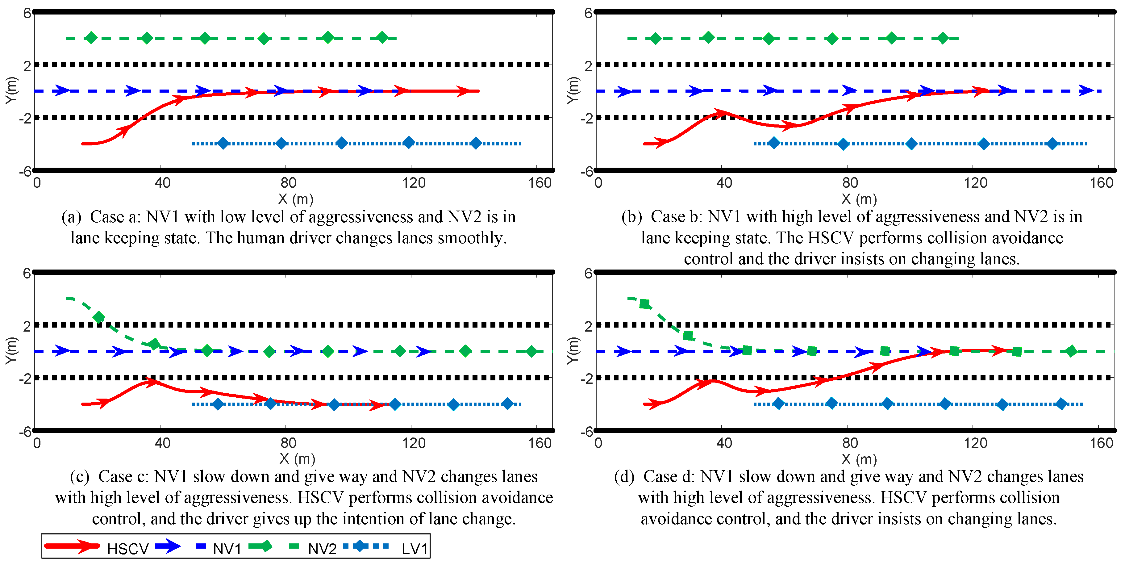
5. Experimental Results and Analysis

HSCVs must share the road with surrounding vehicles in future complex traffic environments, especially in lane change scenarios prone to traffic accidents. The automation control system in an HSCV not only needs to assist the driver in safely changing lanes but also needs to consider how to safely avoid SVs that suddenly change lanes. This section designs two experimental scenarios of HSCV active lane change and HSCV passive avoidance of vehicles that suddenly change lanes to verify the feasibility and effectiveness of the designed safety control scheme, as shown in Figure 5. Scenario 1 shows the impact of NV1’s behavior of slowing down to give way or accelerating to seize the road when the HSCV changes lanes. The dangerous situation of NV2 suddenly changing lanes to compete with the HSCV and occupy the middle lane is considered in Scenario 1. Finally, Scenario 2 demonstrates how a lane-keeping HSCV in a middle lane can safely avoid neighbor vehicles that suddenly change lanes.

Assume that the ego vehicle is an HSCV and all neighbor vehicles of the HSCV are CAVs. All experimental scenarios were simulated in Matlab. The vehicle and driver characteristic parameters are given in Table 2, which include vehicle control input limitations.

Table 3. Parameters of the initial desired state of the vehicle.

Scenario	Driver Intention in HSCV	HSCV	NV1	NV2
$1,2$		${\varphi }_{ref}=0\left(\mathrm{rad}\right),V_{x,exp}=18(\mathrm{m}/\mathrm{s})$	${\varphi }_{ref}=0\left(\mathrm{rad}\right),Y_{ref}=0\left(\mathrm{m}\right)$	${\varphi }_{ref}=0\left(\mathrm{rad}\right)$
$1.a$	Lane change	$Y_{ref}=0\left(\mathrm{m}\right)$	$V_{x,exp}=20(\mathrm{m}/\mathrm{s})$	$Y_{ref}=4\left(\mathrm{m}\right),V_{x,exp}=15(\mathrm{m}/\mathrm{s})$
$1.b$	Lane change	$Y_{ref}=0\left(\mathrm{m}\right)$	$V_{x,exp}=25(\mathrm{m}/\mathrm{s})$	$Y_{ref}=4\left(\mathrm{m}\right),V_{x,exp}=15(\mathrm{m}/\mathrm{s})$
$1.c$	Lane change	$Y_{ref}=0\left(\mathrm{m}\right)$	$V_{x,exp}=16(\mathrm{m}/\mathrm{s})$	$Y_{ref}=0\left(\mathrm{m}\right),V_{x,exp}=25(\mathrm{m}/\mathrm{s})$
$1.d$	Lane change and give up	$Y_{ref}=0\left(\mathrm{m}\right)$	$V_{x,exp}=16(\mathrm{m}/\mathrm{s})$	$Y_{ref}=0\left(\mathrm{m}\right),V_{x,exp}=25(\mathrm{m}/\mathrm{s})$
$2.e$	Lane change	$Y_{ref}=4\left(\mathrm{m}\right)$	$V_{x,exp}=22(\mathrm{m}/\mathrm{s})$	$Y_{ref}=4\left(\mathrm{m}\right),V_{x,exp}=16(\mathrm{m}/\mathrm{s})$
$2.f$	Lane change and give up	$Y_{ref}=4\left(\mathrm{m}\right)$	$V_{x,exp}=22(\mathrm{m}/\mathrm{s})$	$Y_{ref}=4\left(\mathrm{m}\right),V_{x,exp}=25(\mathrm{m}/\mathrm{s})$
$2.g$	Lane keep	$Y_{ref}=0\left(\mathrm{m}\right)$	$V_{x,exp}=22(\mathrm{m}/\mathrm{s})$	$Y_{ref}=4\left(\mathrm{m}\right),V_{x,exp}=18(\mathrm{m}/\mathrm{s})$
$2.h$	Lane keep	$Y_{ref}=0\left(\mathrm{m}\right)$	$V_{x,exp}=25(\mathrm{m}/\mathrm{s})$	$Y_{ref}=4\left(\mathrm{m}\right),V_{x,exp}=18(\mathrm{m}/\mathrm{s})$

displays the initial desired trajectory state and expected vehicle speed of the HSCV and SVs in the above two scenarios. It is worth noting that all lanes have a maximum speed limit of 25 m/s.

5.1. Scenario 1 Test

In Scenario 1, a common HSCV single lane change case was tested, and it was assumed that the lanes of the HSCV, NV1, and NV2 were represented as lane 1, lane 2, and lane 3, respectively. In this designed scenario, the HSCV driver in lane 1 is affected by the low speed of LV1 (assuming it keeps moving forward at a speed of 15 m/s), which leads to the lane-changing behavior of the human driver in the HSCV. Subsequently, in cases a and b, NV2 is set to lane keeping in lane 3, and only the effect of the different responses of NV1 on the HSCV is studied. NV1 in case a has a moderate level of aggressiveness, while NV1 is set with a high level of aggressiveness in case b. Case c and case d are supplements to the first two cases. NV1 is set to a low aggressiveness level, and the impact of the sudden lane changing behavior of NV2 with a high level of aggressiveness on the HSCV is studied. In all cases of Scenario 1, the initial velocities of the HSCV and LV1 are 18 m/s and 15 m/s, respectively, and the initial positions of the HSCV, NV1, NV2, and LV1 are $(15,-4),(0,0),(10,4),(50,-4)$, respectively. The initial velocities of NV1 and NV2 are 20 m/s and 15 m/s in cases a and b, and they are both 16 m/s in cases c and d.

Figure 6, Figure 7 and Figure 8 show the experimental results of vehicle trajectory, vehicle longitudinal speed, and longitudinal position, respectively, under the influence of different driving styles of NV1 and NV2. It can be found that NV1 will slow down and give way when it is in a low or moderate level of aggressiveness. The difference between low-level and moderate-level aggressive NV1 is that the former will maintain a greater distance between vehicles. In case a, the human driver in the HSCV can safely and smoothly change lanes. In case b, high-level aggressive NV1 will accelerate to occupy the road, and the automation control system in the HSCV will modify the driver’s control commands to avoid NV1 safely. As the collision threat caused by the acceleration of NV1 increases, the automation control system gradually decelerates the HSCV and corrects the steering angle to maintain a safe distance from NV1. Until the HSCV safely avoids NV1, it gradually releases control authority to the driver, restores the driver’s desired speed, and assists the driver in changing lanes. Cases c and d show the experimental results that the HSCV automatic control system can ensure the safe avoidance of NV2 under two driving conditions: driver giving up lane change and driver insisting on lane change.

Figure 9 and Figure 10 present the HSCV front steering angle and the curve of the driving control authority between the driver and the automation control system, respectively. In case a, since the safety threat posed by NV1’s deceleration is very small, the automation control system in the HSCV only plays an auxiliary role, and the steering angle of the vehicle is mainly controlled by the driver. Cases b, c, and d show the situation where the SV and HSCV compete for the same lane. The HSCV automation control system will quickly deprive the driver of the control authority and perform safe avoidance until the driver senses the danger and returns to the original road, or it will assist the driver who insists on changing lanes. As shown in Figure 10, the automation control system increases intervention as environmental risks increase, and the driver’s control authority $\lambda$ gradually decreases. After the driver completes the lane change or gives up the lane change, the environmental danger is reduced, and the driver’s control authority $\lambda$ gradually approaches 1.

5.2. Scenario 2 Test

Scenario 2 consists of cases e, f, g, and h and considers HSCV passive avoidance of sudden lane changes by adjacent vehicles. In this scenario, the HSCV, NV1, and NV2 are in lane 2, lane 1, and lane 3, respectively. Faced with the competitive lane change behavior of NV1 to lane 2, the driver in the HSCV may choose to change lanes to avoid collision or slow down to give way. In cases e and f, the impact of the different driving styles of NV2 on the HSCV of passive lane change to road 3 to avoid NV1 was tested. Cases g and h tested the HSCV that insisted on lane keeping and safely avoided the NV1 that changed lanes from different locations. In all cases of Scenario 2, the initial speed of the HSCV and NV2 is set to 18 m/s. The initial speed of NV1 is 16 m/s in cases e and f, while it is 18 m/s in cases f and g. The initial position of the HSCV is $(15,0)$ in all cases of Scenario 2. The initial position of NV1 is $(20,-4)$ in cases e, f, and g and $(5,-4)$ in case h. The initial position of NV2 is $(0,4)$ in cases e and f, while it is $(20,4)$ in cases g and h.

Figure 11, Figure 12 and Figure 13 show the vehicle trajectory, vehicle speed, and vehicle position in Scenario 2. In case e, it can be found that when the aggressiveness level of NV2 in lane 3 is low, the driver in the HSCV can smoothly change lanes to avoid NV1 which suddenly changes lanes to lane 2. Case f supplements case e and tests the situation where NV2 competes with the HSCV for lane 3. As the threat of collision between the HSCV and NV2 increases, the automation control system in the HSCV will intervene in vehicle speed and wheel angle to avoid collision with NV2 until the driver gives up the lane change and desired vehicle speed and returns to the original road at a low speed. Case g shows that the human driver and the HSCV avoid NV1’s lane change by actively slowing down, slightly steering, and gradually returning to the driver’s desired speed after completing the safe avoidance. Case h shows the dangerous situation of NV1 suddenly accelerating and changing lanes from the blind spot behind the HSCV, which is invisible to human drivers. The automation control system in the HSCV performs emergency collision avoidance on NV1 by decelerating and controlling the steering angle until the avoidance is successful and then assists the driver who chooses to follow the leader vehicle at a low speed to maintain lanes.

Figure 14 and Figure 15 show the control of steering angle by the driver and automation system in HSCV and the dynamically allocated driving control authority, respectively. In the case of e, due to NV2 slowing down to give way, HSCV is mainly controlled by the human driver and can change lanes smoothly to avoid NV1, which suddenly changes lanes. However, in case f, NV2 with a high aggressiveness level will bring a higher collision threat. The automated control system in the HSCV will reduce the driver’s control authority until the driver gives up the lane change. Then, the value $\lambda$ of the driver’s control authority will gradually increase to close to 1. In cases g and h, as the collision threat caused by NV1’s sudden lane change increases, HSCV will allocate more driving authority to the automation control system to intervene in driving. The difference between cases g and h is that in case g, the NV1 that changes lanes in front of the HSCV reserves more space for the HSCV to decelerate and avoid collisions without requiring automation system intervention in the steering angle. In contrast to case g, HSCV in case h needs more steering control to avoid collision when facing NV1 changing lanes behind it.

6. Conclusions

This work presents HSCV safety control based on game theory and multi-vehicle interaction. First, a comprehensive driver model integrating steering control and speed control was designed based on the BELCM algorithm. Next, a shared control strategy based on the driving risk field was designed to dynamically adjust the driving control authority between the human driver and the HSCV automation control system. Considering that different driving styles of SVs in the driving environment will have different impacts on the HSCV, two critical indicators of driving safety and travel efficiency were used to define the aggressiveness level of SVs. MPC was used to predict the future status of traffic participants. Finally, the interaction problem between HSCV and SVs was transformed into DMPC, which can be solved through the idea of Nash equilibrium. Two different scenarios were designed to evaluate the performance of the HSCV safety control method. The simulation results show that in HSCV lane changing and lane keeping scenarios, the HSCV shared controller designed in this study can assist human drivers in safely avoiding neighbor vehicles with dangerous behaviors of sudden acceleration and lane changing.

This article mainly focuses on the safety control of HSCVs, and the test of the experimental scenario is based on reasonable assumptions about the driver’s intention to change lanes and deceleration intention. A more realistic integrated driver model that considers steering control and speed control requires us to conduct further research in the future, especially on the impact of driver intention on shared control, to improve shared control technology in HSCVs.

References

1. Guo, H.; Zhang, Y.; Cai, S.; Chen, X. Effects of Level 3 Automated Vehicle Drivers’ Fatigue on Their Take-Over Behaviour: A Literature Review. J. Adv. Transp. 2021, 2021, 1–12. [Google Scholar] [CrossRef]
2. Wang, W.; Na, X.; Cao, D.; Gong, J.; Xi, J.; Xing, Y.; Wang, F.Y. Decision-making in driver-automation shared control: A review and perspectives. IEEE/CAA J. Autom. Sin. 2020, 7, 1289–1307. [Google Scholar] [CrossRef]
3. Bonnefon, J.F.; Shariff, A.; Rahwan, I. The social dilemma of autonomous vehicles. Science 2016, 352, 1573–1576. [Google Scholar] [CrossRef] [PubMed]
4. Ansari, S.; Naghdy, F.; Du, H. Human-machine shared driving: Challenges and future directions. IEEE Trans. Intell. Veh. 2022, 7, 499–519. [Google Scholar] [CrossRef]
5. Pankiewicz, N.; Turlej, W.; Orłowski, M.; Wrona, T. Highway Pilot Training from Demonstration. In Proceedings of the 2021 25th International Conference on Methods and Models in Automation and Robotics (MMAR), Międzyzdroje, Poland, 23–26 August 2021; pp. 109–114. [Google Scholar]
6. Marcano, M.; Díaz, S.; Pérez, J.; Irigoyen, E. A review of shared control for automated vehicles: Theory and applications. IEEE Trans. Hum. Mach. Syst. 2020, 50, 475–491. [Google Scholar] [CrossRef]
7. International, S. Taxonomy and definitions for terms related to driving automation systems for on-road motor vehicles. SAE Int. 2018, 4970, 1–5. [Google Scholar]
8. Sheridan, T.B.; Verplank, W.L.; Brooks, T. Human/computer control of undersea teleoperators. In Proceedings of the NASA Ames Research Center The 14th Annual Conference on Manual Control, Los Angeles, CA, USA, 25–27 April 1978. [Google Scholar]
9. Li, X.; Wang, Y. Shared steering control for human–machine co-driving system with multiple factors. Appl. Math. Model. 2021, 100, 471–490. [Google Scholar] [CrossRef]
10. Saleh, L.; Chevrel, P.; Claveau, F.; Lafay, J.F.; Mars, F. Shared steering control between a driver and an automation: Stability in the presence of driver behavior uncertainty. IEEE Trans. Intell. Transp. Syst. 2013, 14, 974–983. [Google Scholar] [CrossRef]
11. Nguyen, A.T.; Sentouh, C.; Popieul, J.C. Driver-automation cooperative approach for shared steering control under multiple system constraints: Design and experiments. IEEE Trans. Ind. Electron. 2016, 64, 3819–3830. [Google Scholar] [CrossRef]
12. Nguyen, A.T.; Sentouh, C.; Popieul, J.C. Sensor reduction for driver-automation shared steering control via an adaptive authority allocation strategy. IEEE/ASME Trans. Mechatronics 2017, 23, 5–16. [Google Scholar] [CrossRef]
13. Li, R.; Li, Y.; Li, S.E.; Zhang, C.; Burdet, E.; Cheng, B. Indirect shared control for cooperative driving between driver and automation in steer-by-wire vehicles. IEEE Trans. Intell. Transp. Syst. 2020, 22, 7826–7836. [Google Scholar] [CrossRef]
14. Cole, D.; Pick, A.; Odhams, A. Predictive and linear quadratic methods for potential application to modelling driver steering control. Veh. Syst. Dyn. 2006, 44, 259–284. [Google Scholar] [CrossRef]
15. Hang, P.; Zhang, Y.; Lv, C. Brain-Inspired Modeling and Decision-Making for Human-Like Autonomous Driving in Mixed Traffic Environment. IEEE Trans. Intell. Transp. Syst. 2023, 24, 10420–10432. [Google Scholar] [CrossRef]
16. Mulder, M.; Abbink, D.A.; Van Paassen, M.M.; Mulder, M. Design of a haptic gas pedal for active car-following support. IEEE Trans. Intell. Transp. Syst. 2010, 12, 268–279. [Google Scholar] [CrossRef]
17. Abbink, D.A.; Mulder, M.; Van der Helm, F.C.; Mulder, M.; Boer, E.R. Measuring neuromuscular control dynamics during car following with continuous haptic feedback. IEEE Trans. Syst. Man Cybern. Part B (Cybern.) 2011, 41, 1239–1249. [Google Scholar] [CrossRef]
18. Sentouh, C.; Debernard, S.; Popieul, J.C.; Vanderhaegen, F. Toward a shared lateral control between driver and steering assist controller. IFAC Proc. Vol. 2010, 43, 404–409. [Google Scholar] [CrossRef]
19. Alirezaei, M.; Corno, M.; Katzourakis, D.; Ghaffari, A. A robust steering assistance system for road departure avoidance. IEEE Trans. Veh. Technol. 2012, 61, 1953–1960. [Google Scholar] [CrossRef]
20. Erlien, S.M.; Fujita, S.; Gerdes, J.C. Shared steering control using safe envelopes for obstacle avoidance and vehicle stability. IEEE Trans. Intell. Transp. Syst. 2015, 17, 441–451. [Google Scholar] [CrossRef]
21. Xing, Y.; Huang, C.; Lv, C. Driver-automation collaboration for automated vehicles: A review of human-centered shared control. In Proceedings of the 2020 IEEE Intelligent Vehicles Symposium (IV), Las Vegas, NV, USA, 19 October–13 November 2020; pp. 1964–1971. [Google Scholar]
22. Anderson, S.J.; Karumanchi, S.B.; Iagnemma, K.; Walker, J.M. The intelligent copilot: A constraint-based approach to shared-adaptive control of ground vehicles. IEEE Intell. Transp. Syst. Mag. 2013, 5, 45–54. [Google Scholar] [CrossRef]
23. Song, L.; Guo, H.; Wang, F.; Liu, J.; Chen, H. Model predictive control oriented shared steering control for intelligent vehicles. In Proceedings of the 2017 29th Chinese Control And Decision Conference (CCDC), Chongqing, China, 28–30 May 2017; pp. 7568–7573. [Google Scholar]
24. Liu, J.; Chen, H.; Guo, H.; Song, L.; Hu, Y. Moving horizon shared steering strategy for intelligent vehicle based on potential-hazard analysis. IET Intell. Transp. Syst. 2019, 13, 541–550. [Google Scholar] [CrossRef]
25. Huang, C.; Lv, C.; Naghdy, F.; Du, H. Reference-free approach for mitigating human–machine conflicts in shared control of automated vehicles. IET Control Theory Appl. 2020, 14, 2752–2763. [Google Scholar] [CrossRef]
26. Na, X.; Cole, D.J. Linear quadratic game and non-cooperative predictive methods for potential application to modelling driver–AFS interactive steering control. Veh. Syst. Dyn. 2013, 51, 165–198. [Google Scholar] [CrossRef]
27. Na, X.; Cole, D.J. Game-theoretic modeling of the steering interaction between a human driver and a vehicle collision avoidance controller. IEEE Trans. Hum.-Mach. Syst. 2014, 45, 25–38. [Google Scholar] [CrossRef]
28. Li, M.; Song, X.; Cao, H.; Wang, J.; Huang, Y.; Hu, C.; Wang, H. Shared control with a novel dynamic authority allocation strategy based on game theory and driving safety field. Mech. Syst. Signal Process. 2019, 124, 199–216. [Google Scholar] [CrossRef]
29. Yue, M.; Fang, C.; Zhang, H.; Shangguan, J. Adaptive authority allocation-based driver-automation shared control for autonomous vehicles. Accid. Anal. Prev. 2021, 160, 106301. [Google Scholar] [CrossRef] [PubMed]
30. Hang, P.; Lv, C.; Huang, C.; Xing, Y.; Hu, Z. Cooperative decision making of connected automated vehicles at multi-lane merging zone: A coalitional game approach. IEEE Trans. Intell. Transp. Syst. 2021, 23, 3829–3841. [Google Scholar] [CrossRef]
31. Hang, P.; Lv, C.; Huang, C.; Cai, J.; Hu, Z.; Xing, Y. An integrated framework of decision making and motion planning for autonomous vehicles considering social behaviors. IEEE Trans. Veh. Technol. 2020, 69, 14458–14469. [Google Scholar] [CrossRef]
32. Liu, J.; Zhou, D.; Hang, P.; Ni, Y.; Sun, J. Towards Socially Responsive Autonomous Vehicles: A Reinforcement Learning Framework With Driving Priors and Coordination Awareness. IEEE Trans. Intell. Veh. 2024, 9, 827–838. [Google Scholar] [CrossRef]
33. Wang, M.; Hoogendoorn, S.P.; Daamen, W.; van Arem, B.; Happee, R. Game theoretic approach for predictive lane-changing and car-following control. Transp. Res. Part C Emerg. Technol. 2015, 58, 73–92. [Google Scholar] [CrossRef]
34. Wang, J.; Wang, J.; Wang, R.; Hu, C. A framework of vehicle trajectory replanning in lane exchanging with considerations of driver characteristics. IEEE Trans. Veh. Technol. 2016, 66, 3583–3596. [Google Scholar] [CrossRef]
35. Lv, C.; Hu, X.; Sangiovanni-Vincentelli, A.; Li, Y.; Martinez, C.M.; Cao, D. Driving-style-based codesign optimization of an automated electric vehicle: A cyber-physical system approach. IEEE Trans. Ind. Electron. 2018, 66, 2965–2975. [Google Scholar] [CrossRef]
36. MorÉn, C.B.J. Emotional learning: A computational model of the amygdala. Cybern. Syst. 2001, 32, 611–636. [Google Scholar]
37. Dehkordi, B.M.; Parsapoor, A.; Moallem, M.; Lucas, C. Sensorless speed control of switched reluctance motor using brain emotional learning based intelligent controller. Energy Convers. Manag. 2011, 52, 85–96. [Google Scholar] [CrossRef]
38. Motamed, S.; Setayeshi, S.; Rabiee, A. Speech emotion recognition based on a modified brain emotional learning model. Biol. Inspired Cogn. Archit. 2017, 19, 32–38. [Google Scholar] [CrossRef]
39. Orłowski, M.; Wrona, T.; Pankiewicz, N.; Turlej, W. Safe and goal-based highway maneuver planning with reinforcement learning. In Advanced, Contemporary Control: Proceedings of KKA 2020—The 20th Polish Control Conference, Łódź, Poland, 2020; Springer: Berlin/Heidelberg, Germany, 2020; pp. 1261–1274. [Google Scholar]
40. Turlej, W.; Mitkowski, W. Multiple Hypothesis Planning for Vehicle Control. In Proceedings of the XXI Polish Control Conference, Gliwice, Poland, 14 June 2023; Springer: Berlin/Heidelberg, Germany; pp. 245–253. [Google Scholar]
41. Zhang, Z.; Wang, C.; Zhao, W.; Xu, C.; Chen, G. Driving authority allocation strategy based on driving authority real-time allocation domain. IEEE Trans. Intell. Transp. Syst. 2021, 23, 8528–8543. [Google Scholar] [CrossRef]
42. Wang, M.; Wang, Z.; Talbot, J.; Gerdes, J.C. Game-theoretic planning for self-driving cars in multivehicle competitive scenarios. IEEE Trans. Robot. 2021, 37, 1313–1325. [Google Scholar] [CrossRef]
43. Zhang, K.; Wang, J.; Chen, N.; Yin, G. A non-cooperative vehicle-to-vehicle trajectory-planning algorithm with consideration of driver’s characteristics. Proc. Inst. Mech. Eng. Part D J. Automob. Eng. 2019, 233, 2405–2420. [Google Scholar] [CrossRef]
Figure 1. Overall system framework.
Applsci 14 02441 g001
Figure 2. Brain emotional learning circuit model [37].
Applsci 14 02441 g002
Figure 3. Framework of driver model based on BELCM.
Applsci 14 02441 g003
Figure 4. Graph of driving authority allocation strategy.
Applsci 14 02441 g004
Figure 5. Two test scenarios for HSCV safe driving.
Applsci 14 02441 g005
Figure 6. Test results of vehicle driving trajectory in Scenario 1.
Applsci 14 02441 g006
Figure 7. The test results of vehicle speed in Scenario 1: (a) the HSCV changes lanes smoothly; (b) NV1 with a high aggressiveness competes on the road, and the driver in the HSCV insists on changing lanes; (c) NV2 with high aggressiveness level competes on the road, and the driver in the HSCV gives up changing lanes; (d) the human driver insists on changing lanes while competing with NV2.
Applsci 14 02441 g007
Figure 8. The test results of vehicle position in Scenario 1: (a) the HSCV changes lanes smoothly; (b) NV1 with high aggressiveness competes on the road, and the driver in the HSCV insists on changing lanes; (c) NV2 with high aggressiveness level competes on the road, and the driver in the HSCV gives up changing lanes; (d) the human driver insists on changing lanes while competing with NV2.
Applsci 14 02441 g008
Figure 9. Front wheel angle of HSCV in scenario 1: (a) wheel angle in case a; (b) wheel angle in case b; (c) wheel angle in case c; (d) wheel angle in case d.
Applsci 14 02441 g009
Figure 10. Driving control authority allocation for HSCV in scenario 1: (a) driving authority allocation in case a; (b) driving authority allocation in case b; (c) driving authority allocation in case c; (d) driving authority allocation in case d.
Applsci 14 02441 g010
Figure 11. Test results of vehicle driving trajectory in Scenario 2.
Applsci 14 02441 g011
Figure 12. Test results of vehicle speed in Scenario 2: (a) human driver in HSCV changes lanes to avoid NV2; (b) NV2 with high aggressiveness accelerates to occupy road, and human drivers abandon lane changes; (c) HSCV slows down to give way for NV1; (d) NV1 changes lanes behind HSCV, and HSCV executes obstacle avoidance control to give way.
Applsci 14 02441 g012
Figure 13. Test results of vehicle position in Scenario 2: (a) human driver in HSCV changes lanes to avoid NV2; (b) NV2 with high aggressiveness accelerates to occupy road, and human drivers abandon lane changes; (c) HSCV slows down to give way for NV1; (d) NV1 changes lanes behind HSCV, and HSCV executes obstacle avoidance control to give way.
Applsci 14 02441 g013
Figure 14. Front wheel angle of HSCV in Scenario 2: (a) wheel angle in case e; (b) wheel angle in case f; (c) wheel angle in case g; (d) wheel angle in case h.
Applsci 14 02441 g014
Figure 15. Driving control authority allocation for HSCV in Scenario 2: (a) driving authority allocation in case e; (b) driving authority allocation in case f; (c) driving authority allocation in case g; (d) driving authority allocation in case h.
Applsci 14 02441 g015