Using Irradiation-Acquisition Interleaved Time-Integrated Imaging to Assess Delayed Luminescence and the Noise-Laden Residual Spontaneous Photon Emission of Yeast

Featured Application

The approach presented in this work may be applicable to imaging technology relevant to assessing oxidative stress.

Abstract

Delayed luminescence from organisms informs oxidative stress that may be modulable by external stimulations. In the absence of external stress causing delayed luminescence, organisms may produce spontaneous ultraweak photon emission due to the residual oxygen demand. To better understand the oxidative state of an organism, it is desirable to acquire the delayed luminescence to reach the phase wherein the ultraweak photon emission resides. This, however, is challenging due to the significant difference in the order of magnitude of the photon counts between the two types of photon emission. Conventional time-gated measurement requires a high dynamic range to assess the noise-level photon emission, whereas simple long exposure can miss the kinetics of luminescence. There may be a compromise to be made between robustly acquiring the decay kinetics of the delayed luminescence and reliably acquiring the noise-laden spontaneous photon emission. We demonstrate an irradiation-acquisition interleaved time-integrated imaging approach that may enable the reliable acquisition of slow-decay delayed luminescence down to the level of ultraweak photon emission. Repetitive irradiation was interleaved with a gradually increased time of acquisition to assess the integrated time course of the post-irradiation luminescence. Such instrument configuration performed on yeast facilitated the use of time differentiation to assess the delayed luminescence down to the noise-level ultraweak photon emission at the expense of the total time of acquisition.

1. Introduction

The photoinduced light emission from organic materials, including plants, after illumination ceases is often characterized by a weak intensity and a long lifetime that could reach beyond hundreds of seconds [1,2]. Phenomena of this nature are studied in different fields under different terminologies such as “delayed luminescence”, “long-lived phosphorescence”, “persistent luminescence”, etc. [3]. This long-lived emission is associated with the complexity of the material, which controls the meta-stable storage of excitatory energy and the release of photons. Although the underlying mechanism has not yet been fully understood [4], the delayed photon emission from organic materials, including biologically active materials, is generally attributed to originating from the metabolic reaction with oxygen [5]. As such, delayed photon emission may be induced by different biotic and abiotic stresses, such as those by chemicals [6] or some other physical factors [7]. The signatures of the decay kinetics revealed by the delayed luminescence, whether it is prompt decay or slow, thus long-tailed decay [8,9], may also have the potential to serve as a non-invasive means of assessing oxidative health for several applications, including but not limited to agricultural [10,11] or biomedical endpoints [12]. For organic and polymeric materials, it has also been observed that modifying the molecular bonds may prolong the emission’s lifetime from that of conventional organic phosphorescent materials to that of ultra-long organic phosphorescence [13,14]. Studying the material’s characteristics may benefit from a better understanding of the time behavior of the delayed luminescence that would require the dynamic range of the acquisition of the photons to be adequately large to cover both the initial strong and prompt emission post-stimulation or stress and the terminal level of the slower emission that may reach the noise baseline.

Whatever the lifetime governing the photon emission post-stimulation or stress, the delayed luminescence will eventually reduce to a baseline that may be referred to as spontaneous ultraweak photon emission [15]. Spontaneous ultraweak photon emission, which is alternatively called biophoton emission of organic origin [16], provides intriguing information on the biological health of organisms. However, due to its extremely low photon yield, careful instrumental design is required to reliably acquire ultraweak photon emission. The instrumental configuration would need to maximally reject ambient light [17] and realize long-time acquisition [18] to negotiate the random noise of the photo-electric detectors, including photomultiplier tubes [15] or two-dimensional imaging arrays [19] that are inherent to the detector of high sensitivity achieved via thermo-electrical cooling.

To better understand the dynamic and residual oxidative state of an organism, it is desirable to be able to acquire stress-inducible or externally modulable delayed luminescence down to the level of steady-state ultraweak photon emission. This, however, is challenging due to the significantly different scales of photon counts in the two phases of photon emission. The instrumental configuration used for acquiring ultraweak photon emission usually involves a long exposure time, and thus, it would be challenging to acquire the kinetics of delayed luminescence that requires a much faster time scale and gated or time-stamped acquisition. On the other hand, the faster time-gated acquisition of delayed luminescence may not have enough dynamic range to reliably acquire changes in the photon emission when reaching the residual level [20] of ultraweak photon emission, which can be easily buried under the baseline noise of the electronics. These challenges may add to the inconclusive promises of steady-state ultraweak photon emission being used for studying the residual oxidative state of an organism [21]. It is also worth noting that even though the decay of delayed luminescence from an organism will reach a steady noise baseline, the noise baseline may not be random noise or may not contain random noise alone. Instead, the noise baseline could rest at the level of spontaneous ultraweak photon emission, which is challenging to measure using time-gated configurations that are conventional for acquiring the time trace of delayed luminescence. In practice, an imaging system for studying the luminescence of an organism may have to compromise between robustly acquiring the decay kinetics of the delayed luminescence and reliably acquiring the ultraweak spontaneous photon emission.

In this work, we demonstrate an irradiation-acquisition interleaved time-integrated imaging approach that may enable the reliable acquisition of slow-decay delayed luminescence down to the level of steady-state ultraweak photon emission that is noise-laden. Repetitive irradiation was interleaved with gradually increased times of exposure. Such instrumental configuration, demonstrated with yeast as the sample, allows for the assessment of the decay kinetics of the delayed luminescence via the time differentiation of the time-integrated post-irradiation luminescence to reach the level of noise-laden ultraweak photon emission at the expense of the total time of acquisition.

The principle that is intuitive to the proposed approach is illustrated in Figure 1 in the context of what contributes to photon emission post-stimulation, forming delayed luminescence. We denote the pure delayed photon emission (photon flux, or the number of photons per area per time) as $R_{DL}\left(t\right)$ $\left[{\mathrm{c}\mathrm{m}}^{-2}{·\mathrm{s}}^{-1}\right]$. A time integration of the delayed luminescence alone then leads to

$$I_{DL}\left(0⟺t\right)={\int }_0^t{R}_{DL}\left(t\prime \right)dt\prime$$

(1)

We note that $I_{DL}\left(0⟺t\right)$ corresponds to the total number of photons per area that are accumulated over a duration of $\left[0,t\right]$. Therefore $I_{DL}\left(0⟺t\right)$ has a unit of $\left[{\mathrm{c}\mathrm{m}}^{-2}\right]$. However, $I_{DL}\left(0⟺t\right)$ is also a function of time as it is related to the duration $\left[0,t\right]$ over which $R_{DL}\left(t\right)$ is specified at each point of time $t$.

We denote the baseline noise of photon flux acquired by any photo-electronic detector as $R_{noise}\left(t\right)$. The randomness of the electronic noise will be set to zero for the following time-ensembled value of the baseline noise throughout integration that is significantly longer than the characteristic temporal scale of its variance:

$${\int }_t^{t+∆t}{R}_{noise}\left(t\prime \right)dt\prime =⟨R_{noise}\left(t\prime \right)⟩=0$$

(2)

Since delayed luminescence is acquired in the presence of random noise, the acquired photon emission then becomes:

$$R_{DL}^{noise}\left(t\right)=R_{DL}\left(t\right)+R_{noise}\left(t\right)$$

(3)

and the time integration of the acquired photon emission of Equation (3) becomes:

$$I_{DL}^{noise}\left(0⟺t\right)={\int }_0^t{R}_{DL}\left(t\prime \right)dt\prime +⟨R_{noise}\left(t\prime \right)⟩={\int }_0^t{R}_{DL}\left(t\prime \right)dt\prime$$

(4)

Now, let us assume the presence of an ultraweak photon emission $R_{UPE}\left(t\right)$ that is not much different in magnitude than random noise. The ultraweak photon emission $R_{UPE}\left(t\right)$, however, differs from the random noise in that the magnitude of time integration of $R_{UPE}\left(t\right)$ is proportional to the length of the time of integration as is the following:

$${\int }_t^{t+∆t}{R}_{UPE}\left(t\prime \right)dt\prime =⟨R_{UPE}⟩·∆t$$

(5)

Now, the acquired photon luminescence practically contains three components as the following:

$$R_{DL/UPE}^{noise}\left(t\right)=R_{DL}\left(t\right)+R_{UPE}\left(t\right)+R_{noise}\left(t\right)$$

(6)

of which the time integration becomes

$$\begin{gathered} I_{DL/UPE}^{nosie}\left(0⟺t\right)={\int }_0^t{R}_{DL}\left(t^{\prime }\right)d{t}^{\prime }+{\int }_0^t{R}_{UPE}\left(t^{\prime }\right)d{t}^{\prime }+⟨R_{noise}\left(t\prime \right)⟩ \\ ={\int }_0^t{R}_{DL}\left(t\prime \right)dt\prime +⟨R_{UPE}⟩·t \end{gathered}$$

(7)

Then, if the following measurement is available:

$$I_{UPE}^{noise}\left(0⟺t\right)=⟨R_{UPE}⟩·t,$$

(8)

one may obtain the ultraweak photon emission via time differentiation of Equation (8):

$$R_{UPE}\left(t\right)=\frac{d}{dt}\left[I_{UPE}^{noise}\left(0⟺t\right)\right]$$

(9)

and similarly, the pure-traced delayed luminescence can be obtained by time differentiation of the difference between Equations (7) and (8):

$$R_{DL}\left(t\right)=\frac{d}{dt}\left[I_{DL/UPE}^{noise}\left(0⟺t\right)-I_{UPE}^{noise}\left(0⟺t\right)\right]$$

(10)

Therefore, by taking advantage of the time-integrated photon emission, which can be a combination of random noise, baseline ultraweak photon emission, and delayed luminescence, it may be possible to resolve the time integration of delayed luminescence alone. From the time integration of delayed luminescence alone, the delayed luminescence can be resolved via simple time differentiation. The resulting exclusive delayed luminescence may be assessable at the level of the noise-laden ultraweak photon emission.

If we denote that delayed luminescence consists of various phases of decay [3] as the following, then

$$R_{DL}\left(t\right)=\sum A_{n}exp\left(-\frac{t}{{\tau }_n}\right)$$

(11)

where ${\tau }_n$ denotes the time constant of the n-th phase of the delay if assuming simultaneous initiation by the same irradiation and taking an ascending order according to the magnitude of the time constant, i.e., the slower the decay, the greater the number of n. The integration of Equation (11) leads to the following pattern with multiple shoulders or phases of saturation that will occur for substantially different time constants:

$$I_{DL}\left(t\right)=\sum A_n{\tau }_n\left[1-exp\left(-\frac{t}{{\tau }_n}\right)\right]$$

(12)

The time integration of UPE-only will be a linear function of time, whereas the time integration of the delayed luminescence only will reveal patterns of saturation, and the patterns of saturation are likely tapered by the linear increment of the time integration of the spontaneous ultraweak photon emission. Any afterglow of the irradiation introduced to excite delayed luminescence may also leave traces in the time-integrated luminescence.

2. Materials and Methods

2.1. The Instrument Configuration for Time-Integrated Imaging of Delayed Luminescence under Fiber-Delivered Illumination

The system used for time-integrated acquisition of delayed luminescence of yeast sample is illustrated in Figure 2. The imaging system was configured based on a customized light-tight chamber facilitating bottom-loading of the sample, imaging by a CCD camera, and fiber-delivering of photo-irradiation into the light-tight chamber. The light-tight chamber contained an upper segment that held a CCD camera (Pixis-512F, Princeton Instruments, 512 × 512 pixels, 16-bit data resolution, operating temperature −70 °C) and a 4× microscope objective lens. The middle segment of the light-tight chamber contained an annular structure co-centric to the inner volume of the chamber to let through a 320 μm fiber [22] while unblocking the view of the camera in imaging the bottom-loaded sample. The annular structure to position the fiber was fixated to the inner wall of the chamber using an O-ring. The lower segment of the light-tight chamber held the sample platform that could be bottom-loaded. The three segments of the imaging chambers were connected by black rubber tube adaptors that also worked as light-tight seals. The 320 μm fiber for illumination was passed through the upper edge of the rubber seal, which was compressed against the lens module to ensure light tightness. The 320 μm fiber was coupled to a laser-driven light source (LDLS, Energetiq (Wilmington, MA, USA) EQ-99X-FC, 190 nm—2500 nm, coupled to a 230 μm fiber) [23] via a fiber switch (Piezosystemjena (Jena, Germany), 9 × 1, fitted with 200 μm fiber). Since the LDLS of continuous operation lacked a shutter control, the illumination of the sample was controlled by turning ON and OFF the fiber switch. The fiber switch was controlled by a desktop computer (Dell OptiPlex GX520, Windows NT) via a vendor-provided interface. Another desktop computer (Dell Dimension 5150, Windows NT) controlled the CCD imager via a vendor-provided WINSPEC user interface. This control configuration was chosen as it was manageable for the task given the limitation of the hardware settings. And this configuration was the main determinator of the post-operation time as is described in a subsequent section.

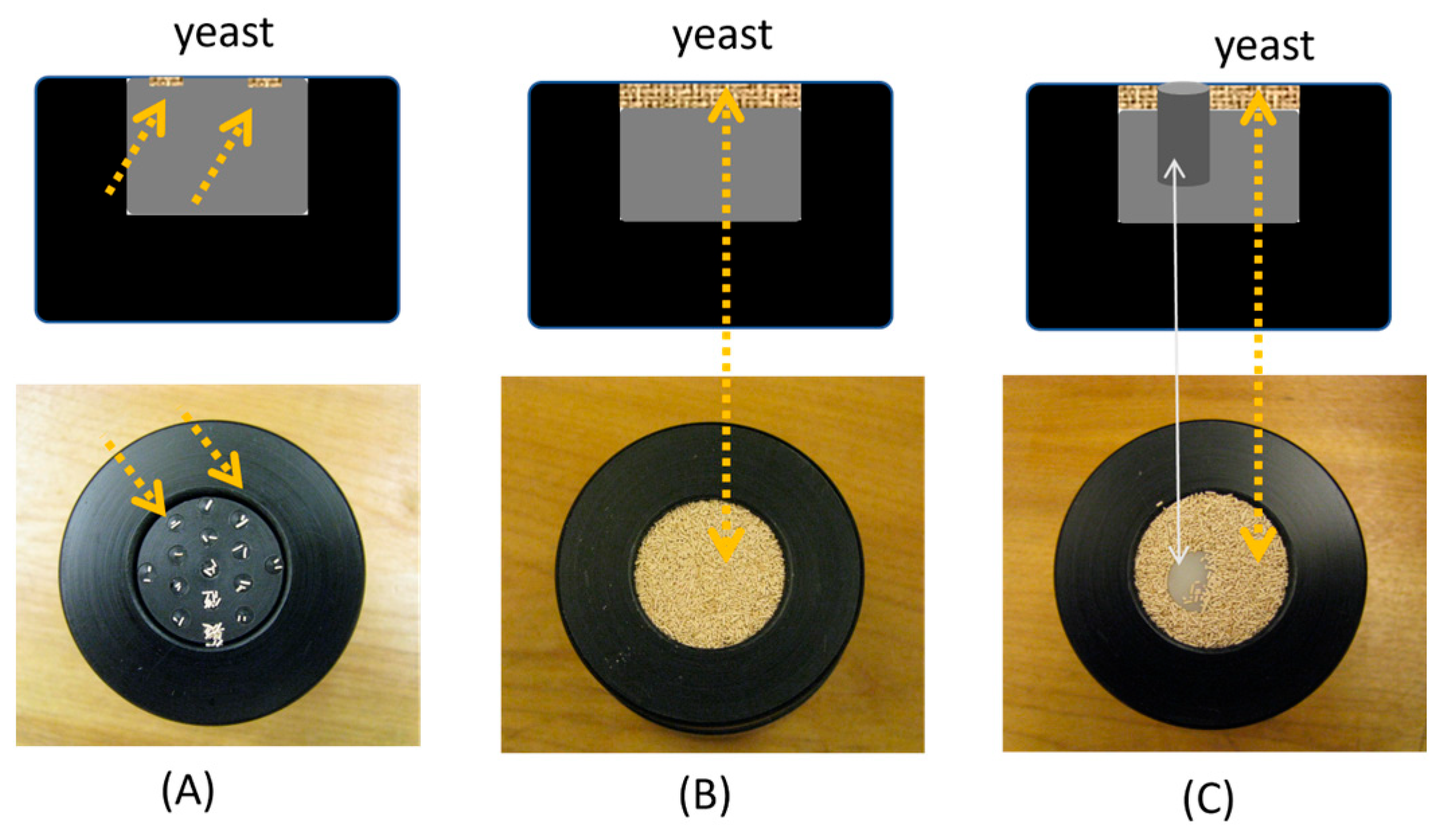
2.2. Sample Holder and the Method of Sample Placement

A master sample holder, as illustrated in Figure 3, was fabricated for the bottom-loading of the sample into the light-tight chamber depicted in Figure 2. The master sample holder had a central receptacle to place a cylindrically shaped bulk sample or another sample platform of a neat-fit cylindrical size for a finer arrangement of the samples. The samples that could be placed in the master holder included reflectance standards (Spectrolum) with reflectivity ranging from 2% to 99%, a custom-fabricated scattering solid-phantom [23], which had a scattering coefficient of 1 mm⁻¹ and an absorption coefficient ranging between [0.005, 0.021] mm⁻¹, and retail yeasts [Fleischmann’s Bread-Machine instant yeast, Walmart Inc., Bentonville, AR, USA]. One sample platform had 16 slightly receded circular pockets on the surface for placing yeast of a specific grain count, up to 16 grains. A few ways that some samples were placed in the sample chamber are exemplified in Figure 3. The imaged area was approximately 2.5 cm in diameter.

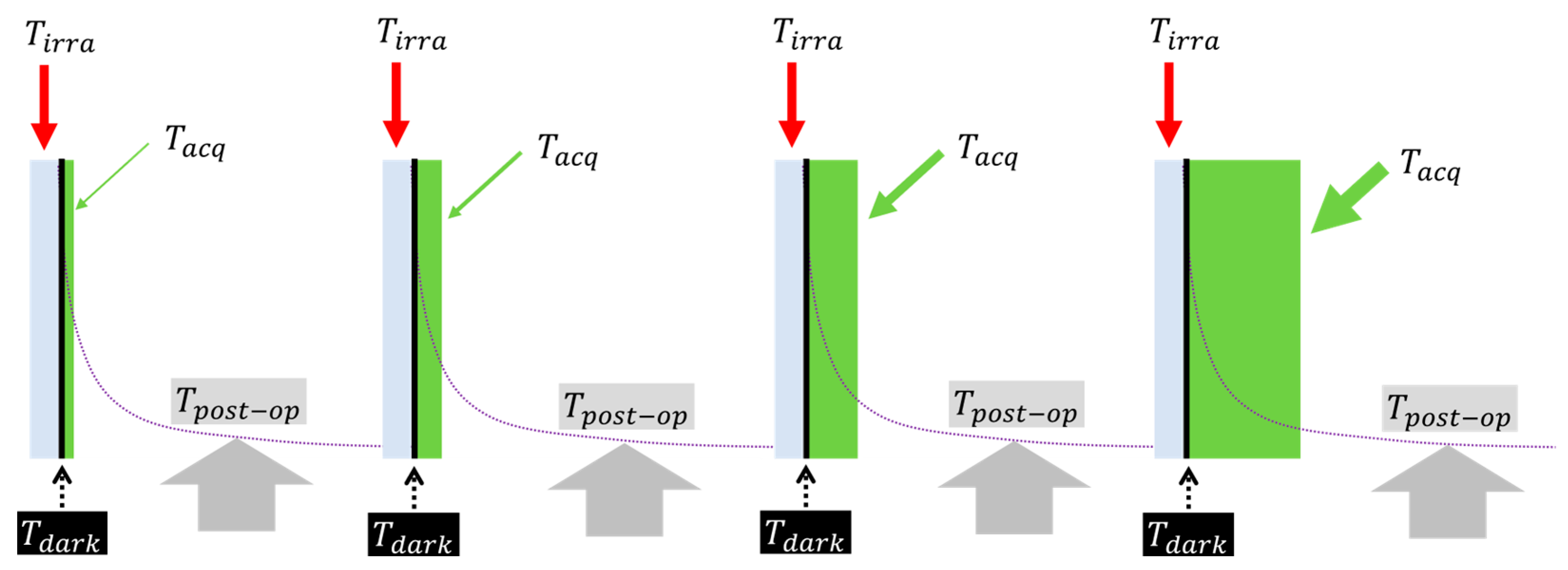
2.3. Time Sequence of the Irradiation-Acquisition Interleaved Imaging

The time sequence of interleaving the irradiation and data acquisition for imaging the delayed luminescence is illustrated in Figure 4. Each cycle contained 4 phases of time: (1) irradiation, (2) dark time, (3) acquisition, and (4) post-operation. The four phases were set for the following functional needs of the proposed approach, which were also dictated by the instrument’s configurability.

(1)

The time of irradiation was the duration of switching on the fiber light delivery via the fiber switch. The fiber-delivered irradiation was switched on for 1 s. The duration of 1 s was determined after experimenting with the time of irradiation of yeasts from as short as 1 ms to as long as 100 s. The 1 s duration provided a good balance between adequate signal-to-noise ratio and non-saturated irradiation, as will be shown in one section of the results.

(2)

The dark time was the time lapse between switching off the fiber light delivery and starting the data acquisition of the CCD camera. A dark time of 20 ms was experimented to be the minimal duration needed to overcome the response lag of the fiber switch to ensure that there was no residual fiber-delivered light to overwhelm the camera once the acquisition of delayed luminescence started. With this dark time, however, there is still a long-lived background afterglow of the fiber-chamber environment to negotiate, as will be revealed in the results.

(3)

The time of acquisition was the exposure time of the CCD imager after dark time. The following numbers were chosen as the acquisition times: 1 to 9 μs at a step of 1 μs, 10 to 90 μs at a step of 10 μs, 100 to 900 μs at a step of 100 μs,1 to 9 ms at a step of 1 ms, 10 to 90 ms at a step of 10 ms, 100 to 900 ms at a step of 100 ms, 1 to 9 s at a step of 1 s, 10 to 90 s at a step of 10 s, 100 to 900 s at a step of 100 s, and 1000 s. Please note that 1 μs was the minimal time of exposure that was configurable for the imager. Additionally, even though the computer user interface of the imager would allow gating operation, the saving function did not allow an autonomous depository of the consecutive imagery that could be acquired by separate but continuous gating of the time sequence of delayed luminescence. In other words, the configurability of the CCD imager interface limited the imaging approach that could be used to obtain the time trace of the delayed luminescence or the time trace of the integration of the delayed luminescence.

(4)

The post-operation time was the time needed to manually operate data saving and re-engaging the fiber switch for the next sequence of a longer time of acquisition than the one completed after the same period of 1 s of irradiation. The manual post-operation was practiced for consistency, taking approximately 10 s. With this 10-s delay between the consecutive measurements, a single sequence of the acquisitions, as specified by Step 3, would take approximately 2.0 h when operated non-stop by one person.

3. Results and Discussions

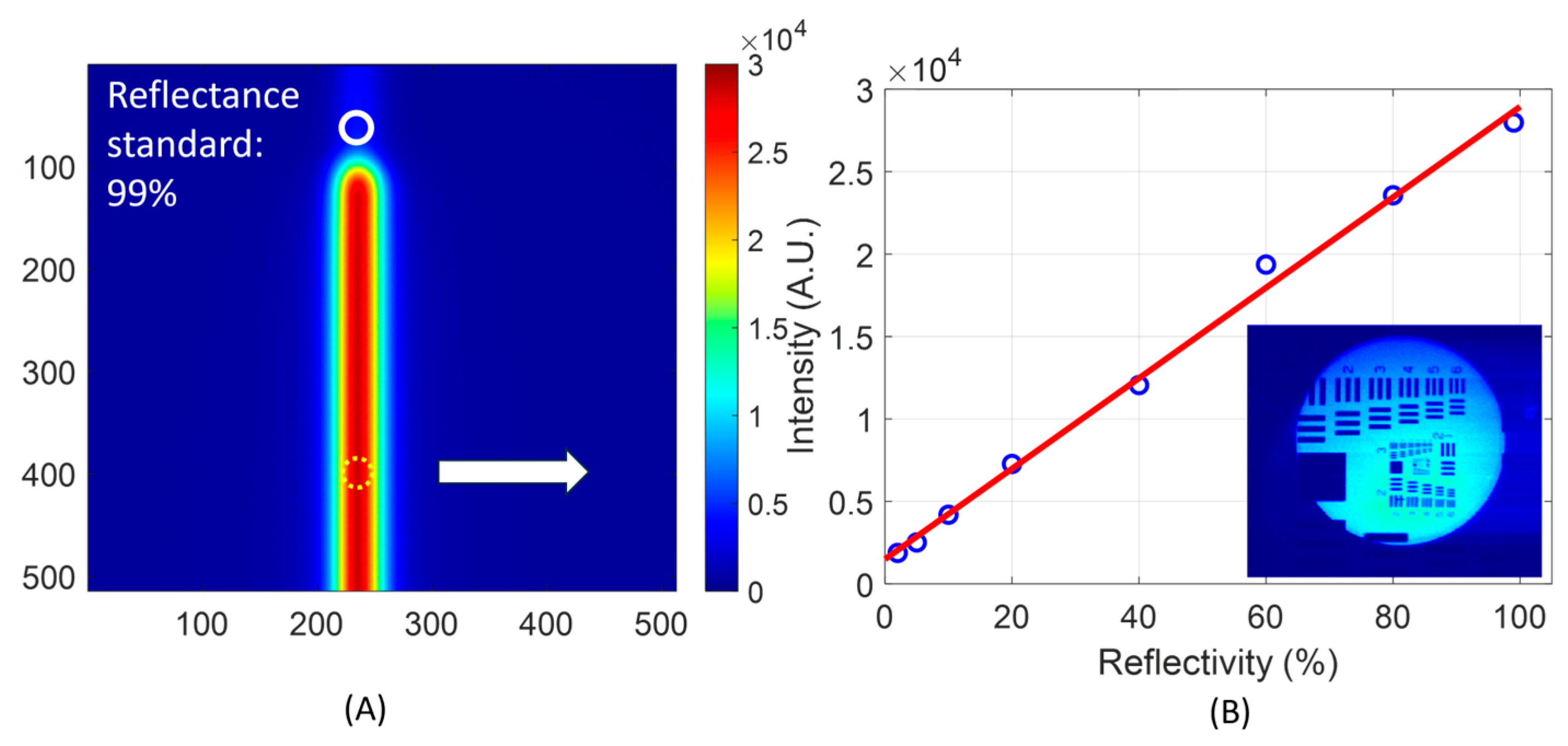
3.1. Basic Benchmarking of the Imaging System

The basic performance of the imaging system in terms of linearly responding to the level of luminescence of a sample at the same duration of acquisition was assessed using reflectance standards of various reflectivity that were exposed to the same level of illumination. The purpose was to examine whether the level of luminescence acquired was precisely proportional to the level of luminescence of the sample chamber since this was the basis for assessing subtle variations of the luminescence over time. An example of the linearity testing result is shown in Figure 5, where the inset at the lower-right corner of Figure 5B illustrates the spatial resolution of the imaging setup. As can be seen from the inset, the imaging plane was focused on the sample surface, which remained consistent with the use of different samples. Keeping the level of the sample surface ensured the consistency of comparing the luminescence from one or multiple configurations of the samples.

The image of Figure 5A was taken from a reflectance standard of 99% reflectivity. The images taken from reflectance standards with the reflectivity ranging from 2% to 80% had a similar pattern of the vertical strip that appeared to be narrower in the shorter length and weaker in intensity than that of 99%. At the top of the vertical strip, there was a relatively faint zone, marked by a white circle in the figure, which corresponded to the projection of the tip of the light-delivery fiber. The vertical strip of which the top edge was tapered was caused by multiple reflections of the light between the flat, diffusively reflective surface of the reflectance standard and the surface of the imaging optics facing the sample. This set of acquisitions was made by tuning ON the irradiation while putting the acquisition time of the CCD imager at 1 μs, the shortest exposure time possible. The light intensity was externally attenuated to ensure that at the 1 μs exposure time, the CCD reading was not saturated by the diffusely reflected light from the reflectance standards of 99% reflectivity. We note that the geometric configuration of the light-delivery fiber with respect to the imaging optics dictated the appearance of the strip in this testing due to the reverberating diffuse reflections from the opposing planar surfaces. However, in the case of imaging, the delayed luminescence from a sample like yeast, no strip-like artifacts were observed.

Replacing the reflectance standards differing in reflectivity in the sample holder was conducted according to the following sequences: (1) bottom-unloading the sample holder, (2) replacing the reflectance standard which would fit into a precise pocket, and (3) bottom-loading the sample holder to the light-tight chamber, then tightening the external harness of the light-tight chamber. The receding structures fabricated into the bottom-loading sample chamber made it possible to make the surface level/orientation of the sample and light-tight conditions consistent throughout the replacement of the eight reflectance standards.

From the images taken with the reflectance standards, the intensity over the same fixed region (20 pixel-lengths along the line orthogonal to the strip, or that the pixels counted would be within the dashed circle at the lower aspect of the strip as shown in Figure 5A) were averaged. The averaged intensity is presented in Figure 5B as a function of the reflectivity of the reflectance standards. Excellent linearity was observed. This linearity indicates that the differentiation of any light intensity acquired by the imager over the same duration of acquisition shall reflect the difference in the luminescence of the sample falling within the collection aperture of the imaging device under otherwise identical conditions. This would ensure that the inter-sample differences in the luminescence are mapped correctly when associated with the same level of irradiation triggering the delayed luminescence. We note that the experimental protocol of interleaved irradiation acquisition involved changing the time of acquisition over a range of 9 orders of magnitude, from 1 μs to 1000 s. The linearity of the acquisition to the length of the duration of acquisition ranging over the 9 orders of magnitude, however, was not assessable due to the lack of a calibrated stable light source that would fit for this task of benchmarking.

3.2. Selection of the Time of Irradiation

The delayed luminescence of the yeast samples when responding to various durations of irradiation and acquired at the same length of the camera exposure is presented in Figure 6. This set of measurements was necessary to determine the length of irradiation, or the relative dose of irradiation that would give an adequate signal-to-noise ratio but not saturate the sample to complicate the time trace of the delayed luminescence. We note that the post-operating time of 10 s between two consecutive irradiation-acquisition cycles unavoidably complicated the time trace of delayed luminescence. The duration of the irradiation, which was controllable with the fiber-switching of the coupling of the delivery fiber to the LSLS light source, was set at the following numbers: 10 ms to 90 ms at an interval of 10 ms, 100 ms to 900 ms at an interval of 100 ms, 1 s to 9 s at an interval of 1 s, and 10 s to 100 s at an interval of 10 s. The time of integration was fixed at 100 s. Therefore, the intensity acquired represented the dose response of the samples. The sample under the irradiation had a solid scattering phantom surrounded by yeasts, and the two types of samples were set at the same surface level. The trace of the red circles in Figure 6A represents the delayed luminescence averaged over the region-of-interest (ROI) corresponding to yeast (the white circle in Figure 6B), whereas the trace of black diamonds in Figure 6A represents the delayed luminescence averaged over the ROI corresponding to the solid scattering phantom (the black circle in Figure 6B). Based on the red trace that corresponds to the luminescence of yeasts when responding to different lengths of irradiation, it was determined that 1 s of the duration of irradiation produced an adequate yield of delayed luminescence without saturating the yeast. Therefore, 1 s was used as the fixed time of irradiation in the subsequent assessment of the delayed luminescence that was acquired at different lengths of the exposure time of the CCD to deduce the time-integrated trace of the luminescence.

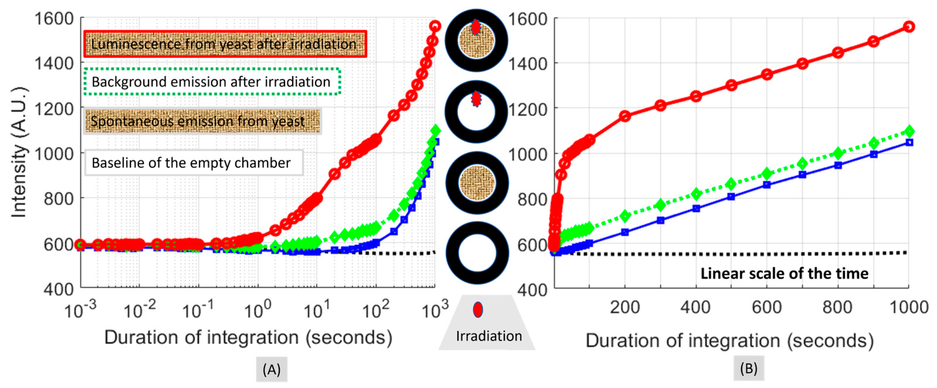
3.3. Time-Integrated Acquisitions at Four Conditions of the Irradiation-Sample Complex

The results shown in Figure 5 and Figure 6 also reveal that any material surface within the FOV of the sample chamber that received the fiber-delivered irradiation and caused multiple or reverberating reflections contributed to the luminescence measured. To acquire delayed luminescence originating specifically from the yeasts, it would be necessary to assess the luminescence of the sample chamber under conditions that would sub-compose the condition of the yeasts post-irradiation. For that purpose, the same irradiation-acquisition interleaved process of acquiring the luminescence from the sample chamber was performed at four conditions of the sample chamber in combination with the prior irradiation. These four conditions and the corresponding level of luminescence acquired as a function of the duration of the integration are given in Figure 7. Figure 7 displayed the same results in a logarithmic scale of the exposure time in (A) and in a linear scale of the exposure time in (B) to better visualize the short-time differences and the long-time patterns, respectively. The four conditions, as stated below, correspond to the four sets in either Figure 7A or Figure 7B that are counted from the bottom-most trace in ascending order.

The bottom-most trace corresponds to a baseline irradiation-acquisition interleaved acquisition with an empty chamber and at no actual irradiation. The second trace from the bottom-most one corresponds to a mock irradiation-acquisition interleaved acquisition from yeasts in the chamber but with no irradiation. The difference between this second trace and the bottom-most one was attributed to the spontaneous photon emission of the yeasts. The third trace from the bottom or the second trace from the top corresponds to the irradiation-acquisition interleaved acquisition from an empty chamber under a normal sequence of irradiation. The difference between this third trace and the bottom-most one was attributed to the afterglow of the illumination-delivery fiber. The fourth trace from the bottom of the topmost trace corresponds to the irradiation-acquisition interleaved acquisition from yeasts in the chamber under a normal sequence of irradiation. The difference between this topmost trace and the bottom-most one was attributable to the combination of delayed photon emission of the yeast, afterglow of the illumination-delivery fiber, and spontaneous photon emission.

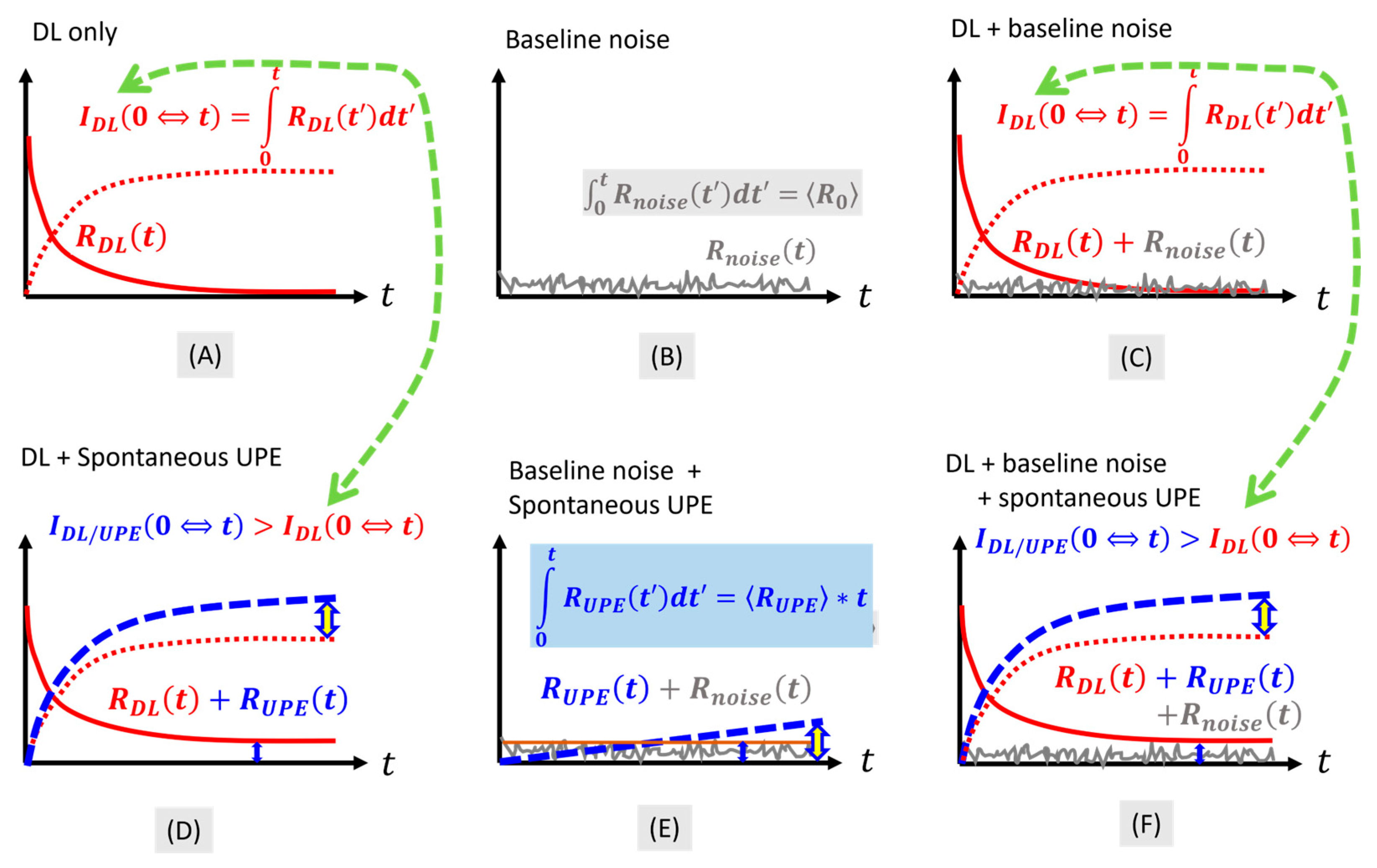
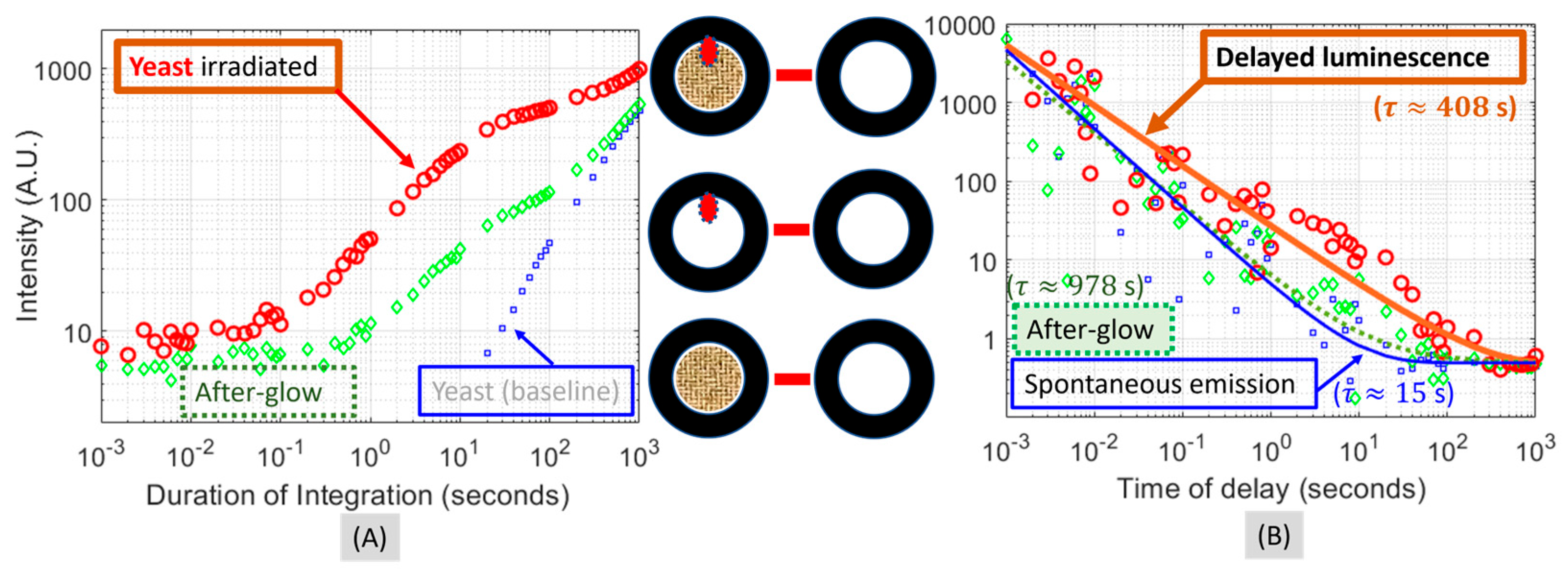
3.4. Time Differentiation of the Time-Integrated Luminescence at Three Conditions of the Sample-Irradiation Setting

The time-integrated luminescence of the three non-baseline conditions shown in Figure 7 are plotted in Figure 8A after subtracting the baseline trace, or the bottom-most trace of Figure 7. The bottom trace marked by the blue squares of the smallest size represents the integration of the spontaneous irradiance from the yeast. As the time of integration increases, this trace, starting noticeably at ~10 s (the smaller values were cut off at the scale), increases steadily at a near-constant slope. The medium trace marked by the green diamonds of the medium size represents the integration of the afterglow irradiance of the illumination-delivery fiber. As the time of integration increases, this trace starts to ascend noticeably at 0.1 s and gradually merges with the bottom trace. The merging of the ascending medium trace with the ascending bottom trace below indicates that the slope of the medium trace was smaller than that of the bottom trace. The top trace marked by the red circles of the largest size represents the integration of the delayed luminescence of the yeast in the presence of the afterglow of the illumination-delivery fiber. This top trace ascends earlier than the medium trace and remains above the medium trace over the entire range of time.

The time differentiation of the time-integrated illuminance of a trace shown in Figure 8A would then correspond to the delayed luminescence at the time of the end of the duration of the integration. The time differentiation results of the three traces of Figure 8A are presented in Figure 8B, with the addition of model-fitting of the respective traces over the time range of 10 μs to 100 s. The three traces were found to be fitted to the following model:

$$R\left(t\right)=A·t^{-b}·exp\left(-\frac{t}{\tau }\right)+\mathsf{\Omega }$$

(13)

The three traces at the descending order, when counted from the top, were fitted by the following models in the form of Equation (13) that gave a goodness-of-fit of 0.92, 0.93, and 0.95, respectively:

$$R_{DL}\left(t\right)=27.48·t^{-0.75}·exp\left(-\frac{t}{407.89}\right)+0.48$$

(14)

$$R_{AG}\left(t\right)=6.32·t^{-0.90}·exp\left(-\frac{t}{977.90}\right)+0.48$$

(15)

$$R_{UPE}\left(t\right)=5.14·t^{-0.98}·exp\left(-\frac{t}{15.32}\right)+0.50$$

(16)

We note that none of the three traces received a good fit using the combination of simple exponential functions indicated by Equation (11). The model form of Equation (13) with which the traces received reasonably good fits contains a hyperbolic function that is multiplied by an exponentially decaying function. Since the hyperbolic function can be expanded to a series of exponentially decaying functions, the model form of Equation (13) is effectively the summation of a series of exponentially decaying functions differing in the rate of temporal decay. This decomposition of a hyperbolic decay trace of a delayed luminescence to multiple phases of exponential decay has been theorized in [3]. One can thus expect that the pattern of the later phase of the luminescence, as depicted in Figure 8B, will be enveloped by an exponential decay with the common or the slowest time constant of the model form of Equation (13). That common time constant may be referred to as a terminal-phase time constant.

The following observations may be made regarding Figure 8B. The bottom-most trace in Figure 8B rests at an apparent residual level of 0.50 (A.U.) after an initial decay of a terminal-phase time constant of 15.32 s. This trace would correspond to the spontaneous photon emission of the yeast when reaching a steady residual value. Comparatively, the medium trace grossly resembles the bottom trace; however, the medium trace reveals a much slower decay with a terminal-phase time constant of 977.90 s and a terminal or residual level not greater than the residual level of the bottom trace. This would correspond to the afterglow of the fiber and the background glow of the chamber excited by the prior fiber-delivered irradiation containing an ultraviolet band. The topmost trace in Figure 8B reveals a decay of a terminal-phase time constant of 407.89 s that descends to the level of the residual value of the bottom-most trace. This topmost trace would correspond to the delayed luminescence of the yeast. To the delayed luminescence of the yeast, the much slower and significantly weaker afterglow would be insignificant in terms of causing any noticeable changes in the temporal course of the delayed luminescence. However, the delayed luminescence would decay to a terminal phase in which the level of the luminescence is even with the residual spontaneous emission of the yeast since no luminescence below the residual level of the spontaneous photon emission would be detectable.

We also note that the terminal phase of the delayed luminescence from one excitation of the single sequence of irradiation acquisition was likely not fully exhausted in the 10 s delay before the next sequence was started. However, under the repetitive settings that differed in only one parameter, which was the time of integration or the duration of acquisition, the difference in the luminescence must represent the effect of that one parameter differing among the repetitive settings. We further note that the method has been demonstrated in measuring the delayed luminescence from a sample like the yeast that was initially significantly stronger than the spontaneous emission to the level of the residual steady-state spontaneous emission. For weaker delayed luminescence such as that would have been associated with a triplet-to-triplet state, this approach may still be applicable; however, the applicability may be compromised by the need to significantly extend the time of integration to accumulate enough photon counts over the noisy baseline. In the case of the sample being made biologically more active than the sample of dry yeast in this work, such as yeast placed in water or with nutrients, one would expect much stronger activities in both the spontaneous residual steady-state photon emission and the delayed luminescence responding to any stress including light. For such sample cases, following the same sequence of interleaved irradiation acquisition will result in a much stronger level of luminescence. With an overall higher level of the time-integrated luminescence to deduce the time differentiation, it may be feasible to resolve finer details of the decay phases of the more active state of the sample in comparison to the dormant state of the sample. Alternatively, the overall stronger luminescence can be probed with a much shorter total time of integration, providing that the terminal-phase time constant is still resolvable by the reduction of the total time of integration.

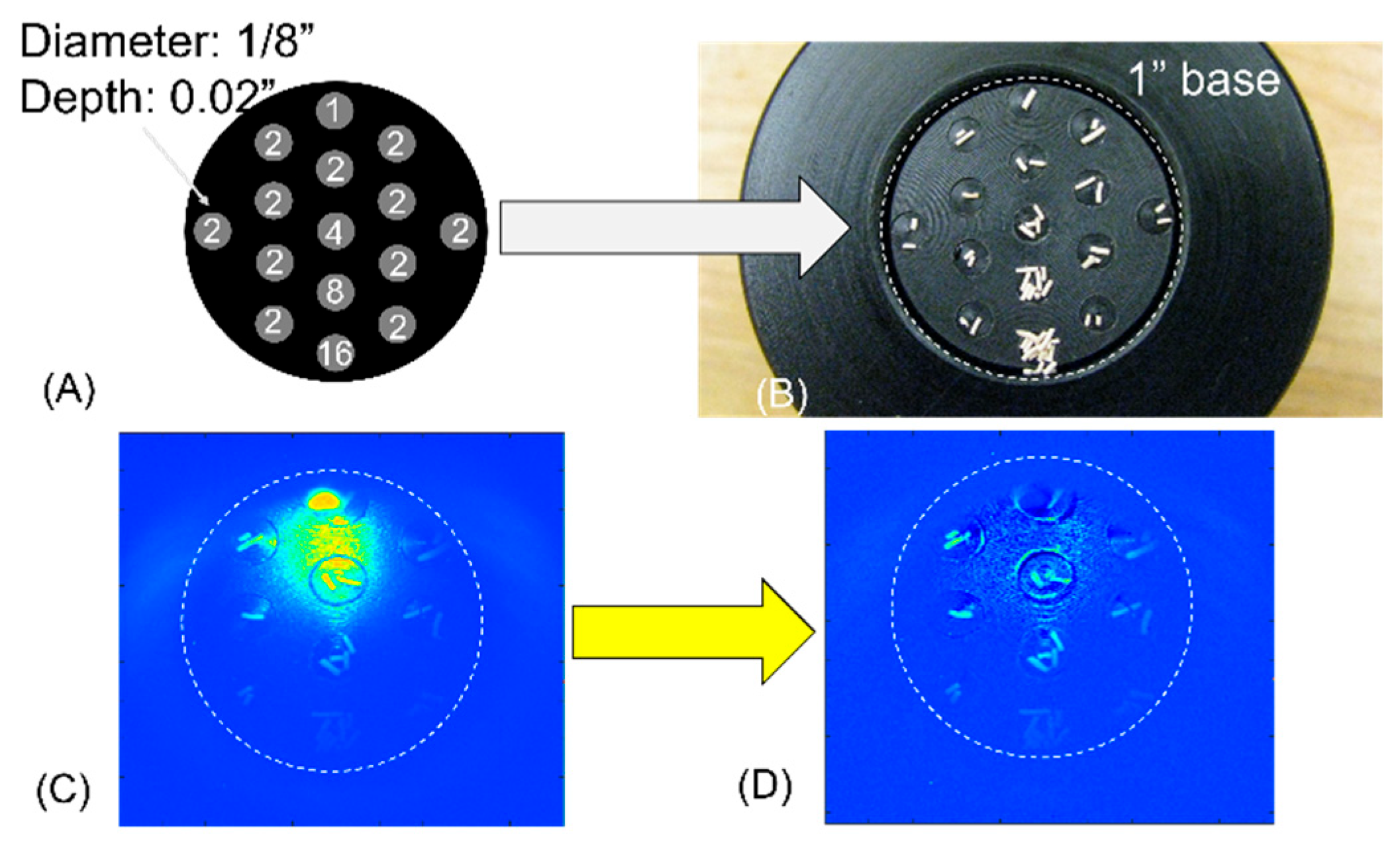
3.5. Spatially Resolved Delayed Luminescence of Individual Grains of The Yeast

An example of the spatially resolved delayed photon emission of the yeast grains in response to photo-irradiation is presented in Figure 9. Grains of the yeast were placed in 16 small cells 1/8″ in diameter that were carved onto a sample platform. Figure 9A shows the layout of the cells, and Figure 9B shows a photograph of the samples placed in the receded cells. The sample platform was held in the custom light-tight chamber for more than 2 h before the illumination. The sample was imaged with the timing sequences shown in Figure 4, up to a total integration time of 1000 s. Figure 9C gave a raw image after the time of integration, wherein the brighter region spreading between the 10 o’clock and the 1 o’clock positions was the residual luminescence of the tip of the fiber after the irradiation to the sample was switched off. That position/extent of the residual luminance of the fiber corresponds to the position of the fiber being reflected by the reflectance standard, as was marked in Figure 5 by the white circle. A baseline image of the integrated background luminescence of the dark chamber was acquired at the same setting, except that no yeast samples were placed in the receded cells. Simple subtraction of the baseline image of the time-integrated acquisition of the empty chamber post-irradiation from the time-integrated acquisition of the yeast-surfaced chamber post-irradiation, as shown in Figure 9C, resulted in Figure 9D, which revealed the delayed luminescence of the individual grains of the yeast. However, the grains of the yeast placed in the cells at the lower 1/3 segment of the FOV were not as clear as those at the middle segment. That was due to the nonuniform irradiation of the light delivered by the fiber to the sample surface that was placed approximately 1″ away from the fiber tip. Additionally, the azimuthal symmetry of the light projected from the fiber was distorted due to the fiber being side-attached to the wall of the sample chamber, which caused wall reflection of the fiber-delivered irradiation. The overall effect was a nonuniform irradiation of or dose to the sample surface, which would cause nonuniform delayed luminescence from the sample of the same photic activity when assessed over the same duration of time after the photic stimulation. Spatially resolved accurate measurement of the true activities of delayed luminescence would require compensating the dose dependency imposed by the nonuniformity of the irradiation.

4. Conclusions

In conclusion, we have demonstrated an irradiation-acquisition interleaved time-integrated imaging to resolve the slow-decay kinetics of delayed luminescence to the level of noise-laden residual spontaneous ultraweak photon emission. To better utilize delayed luminescence for studying the underlying mechanism that may be associated with the dynamic and residual oxidative states of organisms, it will be desirable to acquire the stress-induced delayed luminescence down to the signal level, which may be difficult to differentiate from the noise floor, and to which the steady-state spontaneous photon emission may also be comparable. This, however, is challenging due to the significantly different scales of photon counts in the two types of photon emission. The irradiation-acquisition interleaved time-integrated imaging demonstrated in this work acquired the slow-decay kinetics by first taking integrated acquisition of the kinetics over different lengths of exposure times, then taking the time-derivative of the integrated acquisition. Because integration averages out the random noise and linearly accumulates a weak but steady signal, comparing the difference of the time-integrated luminescence between without and with the irradiation allowed the canceling out of the contribution of both noise and the spontaneous residual photon emission in arriving at a purer trace of the delayed luminescence that could reach to the level of the noise floor. Future works, however, will be necessary to examine if the expense of the total time of acquisition enabling the time of interleaving between acquisition and irradiation may outweigh the benefit of acquiring the delayed luminescence to the phase of spontaneous photon emission that may only be statistically different from the random noise.

References

1. Winkler, R.; Guttenberger, H.; Klima, H. Ultraweak and Induced Photon Emission After Wounding of Plants. Photochem. Photobiol. 2009, 85, 962–965. [Google Scholar] [CrossRef]
2. Footitt, S.; Palleschi, S.; Fazio, E.; Palomba, R.; Finch-Savage, W.E.; Silvestroni, L. Ultraweak Photon Emission from the Seed Coat in Response to Temperature and Humidity—A Potential Mechanism for Environmental Signal Transduction in the Soil Seed Bank. Photochem. Photobiol. 2016, 92, 678–687. [Google Scholar] [CrossRef]
3. Piao, D. On the stress-induced photon emission from organism: II, how will the stress-transfer kinetics affect the photo-genesis? SN Appl. Sci. 2020, 2, 1556. [Google Scholar] [CrossRef]
4. Cifra, M.; Pospíšil, P. Ultra-weak photon emission from biological samples: Definition, mechanisms, properties, detection and applications. J. Photochem. Photobiol. B Biol. 2014, 139, 2–10. [Google Scholar] [CrossRef] [PubMed]
5. Platkov, M.; Tirosh, R.; Kaufman, M.; Zurgil, N.; Deutsch, M. Photobleaching of fluorescein as a probe for oxidative stress in single cells. J. Photochem. Photobiol. B Biol. 2014, 140, 306–314. [Google Scholar] [CrossRef] [PubMed]
6. Kruk, I.; Michalska, T.; Kładna, A.; Berczyński, P.; Aboul-Enein, H.Y. Chemiluminescence investigations of antioxidative activities of some antibiotics against superoxide anion radical. Luminescence 2011, 26, 598–603. [Google Scholar] [CrossRef] [PubMed]
7. Maccarrone, M.; Fantini, C.; Agrò, A.F.; Rosato, N. Kinetics of ultraweak light emission from human erythroleukemia K562 cells upon electroporation. Biochim. Biophys. Acta (BBA)-Biomembr. 1998, 1414, 43–50. [Google Scholar] [CrossRef]
8. Strasser, R.J.; Tsimilli-Michael, M.; Qiang, S.; Goltsev, V. Simultaneous in vivo recording of prompt and delayed fluorescence and 820-nm reflection changes during drying and after rehydration of the resurrection plant Haberlea rhodopensis. Biochim. Biophys. Acta (BBA)-Bioenerg. 2010, 1797, 1313–1326. [Google Scholar] [CrossRef] [PubMed]
9. Oukarroum, A.; Goltsev, V.; Strasser, R.J. Temperature Effects on Pea Plants Probed by Simultaneous Measurements of the Kinetics of Prompt Fluorescence, Delayed Fluorescence and Modulated 820 nm Reflection. PLoS ONE 2013, 8, e59433. [Google Scholar] [CrossRef] [PubMed]
10. Oziembłowski, M.; Trenka, M.; Czaplicka, M.; Maksimowski, D.; Nawirska-Olszańska, A. Selected Properties of Juices from Black Chokeberry (Aronia melanocarpa L.) Fruits Preserved Using the PEF Method. Appl. Sci. 2022, 12, 7008. [Google Scholar] [CrossRef]
11. Gallep, C.D.M.; Robert, D. Time-resolved ultra-weak photon emission as germination performance indicator in single seedlings. J. Photochem. Photobiol. 2020, 1, 100001. [Google Scholar] [CrossRef]
12. Gorączko, W.; Sławiński, J. Secondary Ultraweak Luminescence from Humic Acids Induced by γ-Radiation. Nonlinearity Biol. Toxicol. Med. 2004, 2, 154014204905074. [Google Scholar] [CrossRef]
13. Zhou, B.; Yan, D. Long Persistent Luminescence from Metal–Organic Compounds: State of the Art. Adv. Funct. Mater. 2023, 33, 2300735. [Google Scholar] [CrossRef]
14. Alam, P.; Cheung, T.S.; Leung, N.L.; Zhang, J.; Guo, J.; Du, L.; Kwok, R.T.; Lam, J.W.; Zeng, Z.; Phillips, D.L.; et al. Organic Long-Persistent Luminescence from a Single-Component Aggregate. J. Am. Chem. Soc. 2022, 144, 3050–3062. [Google Scholar] [CrossRef]
15. Kim, J.; Lim, J.; Kim, H.; Ahn, S.; Sim, S.-B.; Soh, K.-S. Scanning Spontaneous Photon Emission From Transplanted Ovarian Tumor of Mice Using a Photomultiplier Tube. Electromagn. Biol. Med. 2006, 25, 97–102. [Google Scholar] [CrossRef] [PubMed]
16. Popp, F.-A.; Li, K.H.; Mei, W.P.; Galle, M.; Neurohr, R. Physical aspects of biophotons. Experientia 1988, 44, 576–585. [Google Scholar] [CrossRef] [PubMed]
17. Burgos, R.C.R.; Červinková, K.; van der Laan, T.; Ramautar, R.; van Wijk, E.P.; Cifra, M.; Koval, S.; Berger, R.; Hankemeier, T.; van der Greef, J. Tracking biochemical changes correlated with ultra-weak photon emission using metabolomics. J. Photochem. Photobiol. B Biol. 2016, 163, 237–245. [Google Scholar] [CrossRef] [PubMed]
18. Gallep, C.M.; Barlow, P.W.; Burgos, R.C.R.; Van Wijk, E.P.A. Simultaneous and intercontinental tests show synchronism between the local gravimetric tide and the ultra-weak photon emission in seedlings of different plant species. Protoplasma 2017, 254, 315–325. [Google Scholar] [CrossRef] [PubMed]
19. Kobayashi, M.; Kikuchi, D.; Okamura, H. Imaging of Ultraweak Spontaneous Photon Emission from Human Body Displaying Diurnal Rhythm. PLoS ONE 2009, 4, e6256. [Google Scholar] [CrossRef] [PubMed]
20. Gałązka-Czarnecka, I.; Korzeniewska, E.; Czarnecki, A.; Sójka, M.; Kiełbasa, P.; Dróżdź, T. Evaluation of Quality of Eggs from Hens Kept in Caged and Free-Range Systems Using Traditional Methods and Ultra-Weak Luminescence. Appl. Sci. 2019, 9, 2430. [Google Scholar] [CrossRef]
21. Lukács, H.; Jócsák, I.; Somfalvi-Tóth, K.; Keszthelyi, S. Physiological Responses Manifested by Some Conventional Stress Parameters and Biophoton Emission in Winter Wheat as a Consequence of Cereal Leaf Beetle Infestation. Front. Plant Sci. 2022, 13, 839855. [Google Scholar] [CrossRef] [PubMed]
22. Piao, D.; McKeirnan, K.L.; Sultana, N.; Breshears, M.A.; Zhang, A.; Bartels, K.E. Percutaneous single-fiber reflectance spectroscopy of canine intervertebral disc: Is there a potential for in situ probing of mineral degeneration? Lasers Surg. Med. 2014, 46, 508–519. [Google Scholar] [CrossRef] [PubMed]
23. Piao, D. Laparoscopic diffuse reflectance spectroscopy of an underlying tubular inclusion: A phantom study. Appl. Opt. 2019, 58, 9689. [Google Scholar] [CrossRef] [PubMed]
Figure 1. Conceptual illustration of the components of photon emission in measuring delayed luminescence. The solid trace refers to a kind of time-varying photon emission, and the dashed line marks the time integration of a kind of time-varying photon emission. (A) Pure delayed luminescence. (B) Random noise over a time duration much longer than its time of variation. (C) Delayed luminescence contaminated with random noise. (D) Delayed luminescence adding to the level of the baseline ultraweak photon emission. (E) Baseline ultraweak photon emission contaminated with random noise. (F) Delayed luminescence adding to the residual ultraweak photon emission contaminated with random noise.
Applsci 14 02392 g001
Figure 2. The system for acquisition of delayed luminescence from a bottom-loaded sample. A laser-driven light source is fiber-guided to a dark chamber for irradiation of the sample. The upper chamber contains an upper segment holding the imaging optics and a CCD camera. The middle chamber contains a structure letting through the 320 μm fiber. The lower segment of the chamber holds the sample. The right panel is an exterior view of the light-tight chamber.
Applsci 14 02392 g002
Figure 3. Top row: the schematic of the master sample holder and the ways of placing samples in the sample holder. Bottom row: The actual samples in the sample holder that can be bottom-loaded to the sample chamber shown in Figure 2. (A) Yeast clusters containing 1–16 grains placed in small cells at a sample platform. (B). Dense clusters of yeast placed on top of a sample platform. (C) A solid scattering phantom was placed amid the dense clusters of yeasts to produce a laterally heterogeneous sample. The arrows mark the corresponding positions or sample-types between a place in the schematic of the top panel and a spot in the photograph of the bottom panel.
Applsci 14 02392 g003
Figure 4. The sequence of interleaving the irradiation and acquisition for repeating the delayed luminescence to be acquired over incrementally increased time of duration of acquisition. The irradiation time was fixed at 1 s. The dark time was fixed at 20 ms. The acquisition time ranged from 1 µs to 1000 s with 10 equal increments over each decade. The post-operation took approximately 10 s. The total sequence in a non-stop mode takes ~2.0 h to complete.
Applsci 14 02392 g004
Figure 5. The response of the imaging system to the luminescence of the sample was measured from reflectance standards differing in reflectivity, under the same illuminance, and acquired at the minimal exposure time (1 us) possible of the CCD imager. (A) shows the image acquired from a reflectance standard of 99% reflectivity. The vertical strip was an artifact that resulted from iterative specular reflection of the diffused light between the surface of the reflectance standard and the imaging optics. The intensity was assessed over two localized regions of approximately 21 pixels each way (horizontally and vertically). One spot was local to the brightest section of the vertical strip, and another spot was beyond the upper tip of the vertical strip, corresponding to the projected position of the illuminating fiber. (B). The intensity assessed at the zone marked by the dashed circle in (A), as a function of the reflectivity of the reflectance standards, is plotted. The inset in (B) shows the focus on the sample surface. The right-pointing arrow in (A) indicates the central spot around which the data corresponding to the plot of (B) were processed.
Applsci 14 02392 g005
Figure 6. Delayed luminescence acquired from yeast over 100 s of exposure time after switching off the irradiation of various durations. The trace of red circles represents the delayed luminescence averaged over the region-of-interest (ROI) corresponding to yeast, whereas the trace of black diamonds represents the delayed luminescence averaged over the ROI corresponding to the solid scattering phantom. The small red elliptical spot at approximately 1 o’clock position represents the residual luminescence (afterglow) of the illumination-delivery fiber.
Applsci 14 02392 g006
Figure 7. Delayed luminescence acquired at four different conditions of the yeast sample and irradiation. (A,B) are the same set of data presented in the logarithmic scale of the abscissa to reveal the patterns happening at times less than 1 s and times greater than 100 s. There are four traces of measurements corresponding to four sets of sample/irradiation combinations. The middle panel illustrates the differences among the four sets using the four annual shapes. The white inner area of the annular shape represents an empty sample chamber. The dense grid-like inner area of the annular shape represents yeast as the sample. The red dot at the 12 o’clock position of the annular shape represents irradiation via the fiber prior to the acquisition of the luminescence from the chamber. The data presented were the average over three sequences performed independently.
Applsci 14 02392 g007
Figure 8. (A) The difference between each of the three non-baseline traces of Figure 7 and the baseline trace. (B) The time differentiation of the three traces shown in (A) with the addition of model fit.
Applsci 14 02392 g008
Figure 9. Imaging of the delayed luminescence of individual grains of yeast. (A) The number of grains placed in each of the receded cells. (B) Photograph of the yeast grains placed in the receded cells. (C) Raw image of the delayed luminescence showing the stronger residual luminescence of the tip of the illuminating fiber that overwhelmed the weak delayed luminescence from the yeast grains. (D) Individual grains in the region-of-interest of (C) that was overwhelmed by the strong residual luminescence of the fiber tip were made to appear after subtracting the baseline luminescence (not shown) that differed from the setting of (C) in only the presence of the grains of yeast.
Applsci 14 02392 g009
Disclaimer/Publisher’s Note: The statements, opinions and data contained in all publications are solely those of the individual author(s) and contributor(s) and not of MDPI and/or the editor(s). MDPI and/or the editor(s) disclaim responsibility for any injury to people or property resulting from any ideas, methods, instructions or products referred to in the content.