Field Telemetry Drilling Dataset Modeling with Multivariable Regression, Group Method Data Handling, Artificial Neural Network, and the Proposed Group-Method-Data-Handling-Featured Artificial Neural Network

Abstract

This paper presents data-driven modeling and a results analysis. Group method data handling (GMDH), multivariable regression (MVR), artificial neuron network (ANN), and new proposed GMDH-featured ANN machine learning algorithms were implemented to model a field telemetry equivalent mud circulating density (ECD) dataset based on surface and subsurface drilling parameters. Unlike the standard GMDH-ANN model, the proposed GMDH-featured ANN utilizes a fully connected network. Based on the considered eighteen experimental modeling designs, all the GMDH regression results showed higher R-squared and minimum mean-square error values than the multivariable regression results. In addition, out of the considered eight experimental designs, the GMDH-ANN model predicts about 37.5% of the experiments correctly, while both algorithms have shown similar results for the remaining experiments. However, further testing with diverse datasets is necessary for better evaluation.

1. Introduction

Swab and surge pressures are created during the drill string tripping out and into the wellbore, respectively. The magnitude of the hydrostatic pressure fluctuation due to the swab/negative and surge/positive depends on, among others, the tripping speed. An unoptimized tripping speed may induce wellbore instability, leading to well collapse or formation fracturing, as well as control issues, which increase the nonproductive time (NPT) and hence the overall drilling budget. The precise prediction of well pressures is crucial, especially in deep-water and horizontal drilling, where a narrow well stability margin poses significant challenges. In addition to tripping speed, fluid properties, geometry, eccentricity, and flow rates also control the well pressure. Moreover, the prediction of the optimum maximum and minimum tripping speeds reduces undesired nonproductive times.

Over the years, researchers have conducted numerous studies of swab and surge phenomena during tripping in and out of the wellbore. They have conducted several experiments and also developed various models based on assumptions such as steady-state and transient conditions, non-slip at the wall, different flow scenarios, fluid rheological properties, well configurations, and operational parameters. Amir et al. (2022) [1,2] extensively reviewed existing swab and surge models, including contributions from Burkhardt (1961) [3], Schuh (1964) [4], Fontenot and Clark (1974) [5], Mitchell (1988) [6], Ahmed (2008) [7], Crespo (2010) [8], Srivastav (2012) [9], Gjerstad (2013) [10], Tang (2016) [11], Fredy (2012) [12], Erge (2015) [13], He (2016) [14], Evren M. (2018) [15], Ettehadi (2018) [16], Shwetank (2020) [17,18], Zakarya (2021) [19], and Amir et al. (2023) [20]. However, these models did not consider all the parameters that affect the swab and surge, and their applicability to estimate experimental data is limited to the specific assumptions and setup conditions.

During drilling and tripping operations, the well pressure is normally determined by the hydrostatic pressure and by the pressure loss due to fluid flow. The equivalent circulation density in specific gravity (sg) is given as (Mitchel et al., 2011) [21]:

$$\mathrm{ECD}={\mathsf{\rho }}_{\mathrm{static}}+\frac{\Delta {\mathrm{P}}_{\mathrm{annulus}}}{0.0981.\mathrm{TVD}}$$

(1)

where $\Delta {\mathrm{P}}_{\mathrm{annulus}}$ is the pressure loss (bar) in the annulus due to fluid flow and ρ_static is the static drilling fluid density (sg). TVD is the true vertical depth (m).

The pump pressure is also determined from the pressure losses across circulation flowlines. The pressure loss in the annulus is given as (Mitchel et al., 2011) [21].

$$\Delta {\mathrm{P} }_{\mathrm{annulus}}=\frac{2{\mathrm{f}\mathsf{\rho }\mathrm{V}}_{\mathrm{Q}}^2}{{\mathrm{D}}_{\mathrm{H}}}\mathrm{L}$$

(2)

where V_Q = Q/A is the velocity of the fluid flow, D_H is the hydraulic fluid flow through the annulus (D_Well–D_Pipe), L is the length of the flow line, and f is the friction factor.

The friction factor f is a function of the Reynolds number, and the surface roughness is given by Haaland (1983) [22]:

$$\frac{1}{\sqrt{\mathrm{f}}}=-1.8\log \left[{\left(\frac{\mathsf{\epsilon }/\mathrm{D}}{3.7}\right)}^{1.11}+\frac{6.9}{\mathrm{Re}}\right]$$

(3)

where ε is the surface roughness coefficient (ε = k/d), k is the surface roughness, and D is the diameter of the pipe.

The friction factor parameter is sensitive, and its prediction is difficult as it is a profile. The theoretical calculation of pressure losses in a wellbore requires knowledge of fluid properties at various temperatures and the shear rates as the fluid flows through each interval of a borehole.

To determine the rheological properties of the drilling fluids and the ECD, there are several models available in the industry’s commercial software. Despite the availability of various mathematical, empirical, and physics-based models currently used in the drilling and well construction sector, incidents related to swab and surge pressures continue to occur. The comparisons of field-measured data with the hydraulic well-flowing models showed discrepancies, and the model required a calibration factor based on measured data (Lohne et al., 2008) [23]. Simulation studies conducted by Amir et al., 2023 [24] showed that the swab and surge prediction of the models were inconsistent and deviated from each other for the considered experimental setup.

In recent years, the application of data-driven modeling has been employed in various sectors, including petroleum drilling. There are several machine learning modeling algorithms. For instance, Amir et al. (2022, 2023) [24,25] utilized machine learning techniques (i.e., linear regression, multivariable regression (MVR), Random Forest, ANN, long-short-term memory (LSTM), and XGboost models) to predict the tripping and drilling operation’s equivalent circulating mud density (ECD), and the results showed satisfactory performance.

In the petroleum industry, among others, ANN algorithms have been applied for prediction such as ROP (Reda Abdel Azim (2020) [26], Ramin Aliyev (2019) [27]), ECD (Husam H. Alkinani (2020) [28], Amir et al., 2021 [24,25]), drilling speed (Ahmad Al-Abduljabbar et al. (2020) [29]), and drilling-fluid-rheological-parameter real-time prediction (Khaled Al-Azani et al. (2018) [30]). In addition, A. Alnmnr (2024) implemented machine learning to investigate Swell Mitigation [31]. RP Ray (2023) studied the importance of data integration in Geotechnical Engineering [32]. E. Gurina (2022) deployed machine learning techniques to predict dysfunctional events in drilling and wells [33].

A literature review indicates the application of the Group Method of Data Handling (GMDH) technique across diverse fields. GMDH is an extended version of multivariable regression that contains non-linear interacting terms. Among others, GMDH has been utilized for accurate log interval value estimation (Mohammed Ayoub (2014) [34]), permeability prediction by Alvin K. Mulashani (2019) [35] and Lidong Zhao (2023) [36], as well as permeability modeling and pore pressure analysis by Mathew Nkurlu (2020) [37]. Additionally, GMDH finds applications in cement compressive strength design (Edwin E. Nyakilla, 2023 [38]), rock deformation prediction (Li et al., 2020 [39]), bubble point pressure estimation by Fahd Saeed Alakbari (2022) and Mohammad Ayoub (2022) [40,41], gas viscosity determination, CO₂ emission modeling (Rezaei et al., 2020 and 2018 [42,43]), the prediction of CO₂ adsorption by Zhou L. (2019) [44] and Li (2017) [45], forecasting stock indices, and modeling power and torque as demonstrated by Ahmadi (2015) [46] and Gao Guozhong (2023) [47], and the prediction of pore pressure by Mgimba (2023) [48].

The GMDH neural network architecture is not as fully connected as that of the commonly used ANN. The modeling performance of the GMDH network in comparison with that of the ANN model is presented in several publications including André et al., 2012 [49]; Bernard et al., 2020 [50]; Ahmadi et al., 2015 [46]; Rezaei et al., 2015 [43].

This study aimed to implement four machine learning algorithms on field drilling data. The first study compared MVR with GMDH to assess the impact of the non-linear interacting features that GMDH has on model prediction. The second study proposed new GMDH-method-generated features that can be utilized as inputs for deep-learning (ANN) modeling, and the networks were fully connected. Then, the newly proposed GMDH-ANN method was compared with a standard ANN that did not include interacting terms. Finally, empirical models were derived from field drilling data by using GMDH and MVR methods.

2. Methodology

The typical machine learning modeling workflow comprises three parts, namely data processing, modeling, and model accuracy performance evaluations. This section presents the details of the description of the dataset and the machine modeling algorithms.

2.1. Description of the Dataset

In this study, therefore, field drilling data acquired through a high-speed (wired drill pipe) telemetry system was used for modeling equivalent circulating density (ECD) based on drilling parameters. Data quality determined the model accuracy performance of the data-driven machine learning modeling. Therefore, the raw data was preprocessed to ensure cleanliness and appropriate feature selection using a correlation heat map to meticulously identify the most suitable features for the modeling process.

2.2. Description of the Machine Learning Algorithms

This section presents the description of the machine learning algorithms implemented in this study that included multivariable regression (MVR), GMDH, ANN, and the proposed fully connected GMDH-featured ANN.

2.2.1. Multivariate Regression

In statistical analysis, researchers actively employ MVR to generate a relationship between the multiple independent variables ${\mathrm{x}}_1,{\mathrm{x}}_2,{\mathrm{x}}_3, \dots ,{\mathrm{x}}_{\mathrm{n}}$, and a single dependent variable ${\mathrm{y}}_{\mathrm{i}}$ (Prentice, 1981) [51]. This technique holds significance in fields where several factors concurrently influence an outcome. MVR has been implemented in several fields and in the petroleum industry. Among others, Amir et al. (2022) [21] applied the method on the field tripping-out dataset.

In this paper, MVR related independent drilling variables/features to predict the target variable, y (ECD). The multiple linear regression model represented the linear combination of weighted features and is expressed as (Anderson T.W., 2003) [52]:

$${\mathrm{y}}_{\mathrm{i}}={\mathsf{\beta }}_0+{\mathsf{\beta }}_1{\mathrm{x}}_1+\dots +{\mathsf{\beta }}_{\mathrm{n}}{\mathrm{x}}_{\mathrm{n}}+\mathsf{\epsilon }$$

(4)

Here, ${\mathrm{y}}_{\mathrm{i}}$ is a dependent variable representing ECD, while ${\mathrm{x}}_1,{\mathrm{x}}_2,{\mathrm{x}}_3,\dots { \mathrm{x}}_{\mathrm{n}}$ different surface and downhole parameters. In Equation (1), β₀ represents the y-intercept (the value of y when all other independent variables are set to 0), β₁ denotes the regression coefficient of the first independent variable ${\mathrm{x}}_1$, ${\mathsf{\beta }}_{\mathrm{n}}$ represents the regression coefficient of the last independent variable ${\mathrm{x}}_{\mathrm{n}}$, and ε is the model error (that describes the degree of variation from the estimate of ${\mathrm{y}}_{\mathrm{i}}$).

The MVR equation can be represented in a concise framework that relates the target, regression variables, regression coefficients, and random errors in the form:

$${\mathrm{y}}_{\mathrm{i}}=\mathrm{X}\mathsf{\beta }+\mathsf{\epsilon }$$

(5)

The model in matrix form can be represented as:

$$\left[\begin{array}{c}{\mathrm{y}}_1\\ {\mathrm{y}}_2\\ ⋮\\ {\mathrm{y}}_{\mathrm{N}}\end{array}\right]=\left[\begin{array}{ccccc}1& {\mathrm{x}}_{11}& \dots & \dots & {\mathrm{x}}_{1\mathrm{M}}\\ 1& {\mathrm{x}}_{21}& \dots & \dots & {\mathrm{x}}_{2\mathrm{M}}\\ ⋮& ⋮& ⋮& ⋮& ⋮\\ 1& {\mathrm{x}}_{\mathrm{N}1}& \dots & \dots & {\mathrm{x}}_{\mathrm{NM}}\end{array}\right]\left[\begin{array}{c}{\mathsf{\beta }}_0\\ {\mathsf{\beta }}_1\\ ⋮\\ {\mathsf{\beta }}_{\mathrm{N}}\end{array}\right]+\left[\begin{array}{c}{\mathsf{\epsilon }}_1\\ {\mathsf{\epsilon }}_2\\ ⋮\\ {\mathsf{\epsilon }}_{\mathrm{N}}\end{array}\right]$$

(6)

Here ${\mathrm{y}}_{\mathrm{i}}$ represents a column vector of the observed values (ECD), $\mathrm{X}$ denotes a matrix of independent variables (each column represents a different drilling variable), $\mathsf{\beta }$ represents a column vector of coefficients, and $\mathsf{\epsilon }$ a column vector of errors.

The optimized set of coefficients. $\left({\mathsf{\beta }}_0,{\mathsf{\beta }}_1,\dots ,{\mathsf{\beta }}_{\mathrm{n}}\right)$ that minimizes the sum of squared differences between the observed ${\mathrm{y}}_{\mathrm{i}}$ and predicted values from the regression function is described in Equation (4).

$$\mathrm{S}\mathrm{S}\mathrm{R}=\underset{{\mathsf{\beta }}_0,{\mathsf{\beta }}_1,\dots ,{\mathsf{\beta }}_{\mathrm{n}}}{\mathrm{m}\mathrm{i}\mathrm{n}} \sum _{\mathrm{i}=1}^{\mathrm{N}} {\left({\mathrm{y}}_{\mathrm{i}}-\left({\mathsf{\beta }}_0+{\mathsf{\beta }}_1{\mathrm{X}}_{1\mathrm{i}}+{\mathsf{\beta }}_2{\mathrm{X}}_{2\mathrm{i}}+\dots +{\mathsf{\beta }}_{\mathrm{n}}{\mathrm{X}}_{\mathrm{n}\mathrm{i}}\right)\right)}^2$$

(7)

The solution involves minimizing the sum of squared errors, leading to the estimated coefficients:

$$\hat{\mathsf{\beta }}={\left({\mathrm{X}}^{\mathrm{T}}\mathrm{X}\right)}^{-1}{\mathrm{X}}^{\mathrm{T}}{\mathrm{y}}_{\mathrm{i}}$$

(8)

Here, $\hat{\mathsf{\beta }}$ is the vector of estimated coefficients$\left({\hat{\mathsf{\beta }}}_0,{\hat{\mathsf{\beta }}}_1,\dots ,{\hat{\mathsf{\beta }}}_{\mathrm{n}}\right)$, ${\mathrm{X}}^{\mathrm{T}}$ is the transpose of matrix $\mathrm{X}$, and ${\left({\mathrm{X}}^{\mathrm{T}}\mathrm{X}\right)}^{-1}$ is the inverse of the product of the transpose of $\mathrm{X}$ and $\mathrm{X}$.

The estimated coefficients are plugged back into the original equation, yielding the final multiple regression equation:

$$\mathrm{E}\hat{\mathrm{C}}\mathrm{D}={\hat{\mathsf{\beta }}}_0+{\hat{\mathsf{\beta }}}_1{\mathrm{X}}_1+{\hat{\mathsf{\beta }}}_2{\mathrm{X}}_2+\dots +{\hat{\mathsf{\beta }}}_{\mathrm{n}}{\mathrm{X}}_{\mathrm{n}}$$

(9)

2.2.2. Group Method Data Handling (GMDH) Algorithm

Alexey G. Ivakhnenko [53] developed GMDH in 1971 as a self-organizing artificial neural network (ANN) for modeling complex systems with multiple variables and nonlinear relationships between inputs and outputs. The relationship between the output and input variables is mathematically described using a process called the Kolmogorov–Gabor polynomial [53]:

$$\begin{array}{c}\mathrm{y}={\mathrm{a}}_0+{\displaystyle \sum _{\mathrm{i}=1}^{\mathrm{n}}} {\mathrm{a}}_{\mathrm{i}}{\mathrm{x}}_{\mathrm{i}}+{\displaystyle \sum _{\mathrm{i}=1}^{\mathrm{n}}} {\displaystyle \sum _{\mathrm{j}=1}^{\mathrm{n}}} {\mathrm{a}}_{\mathrm{i}\mathrm{j}}{\mathrm{x}}_{\mathrm{i}}{\mathrm{x}}_{\mathrm{j}}+{\displaystyle \sum _{\mathrm{i}=1}^{\mathrm{n}}} {\displaystyle \sum _{\mathrm{j}=1}^{\mathrm{n}}} {\displaystyle \sum _{\mathrm{k}=1}^{\mathrm{n}}} {\mathrm{a}}_{\mathrm{i}\mathrm{j}\mathrm{k}}{\mathrm{x}}_{\mathrm{i}}{\mathrm{x}}_{\mathrm{j}}{\mathrm{x}}_{\mathrm{k}}+\dots \\ \end{array}$$

(10)

In Equation (7), $\mathrm{n}$ represents the number of input variables, $\left({\mathrm{x}}_1,{\mathrm{x}}_2,\dots ,{\mathrm{x}}_{\mathrm{n}}\right)$ stands for the input features, and ($\left.{\mathrm{a}}_0,{\mathrm{a}}_1,\dots ,{\mathrm{a}}_{\mathrm{n}}\right)$ the coefficients. The Kolmogorov–Gabor polynomial arrangement involving only two parameters can be expressed as [53]:

$${\hat{\mathrm{y}}}_{\mathrm{i}}={\mathrm{a}}_{\mathrm{o}}+{\mathrm{a}}_1{\mathrm{x}}_{\mathrm{i}}+{\mathrm{a}}_2{\mathrm{x}}_{\mathrm{j}}++{\mathrm{a}}_3{\mathrm{x}}_{\mathrm{i}}^2+{\mathrm{a}}_4{\mathrm{x}}_{\mathrm{j}}^2+{\mathrm{a}}_5{\mathrm{x}}_{\mathrm{i}}{\mathrm{x}}_{\mathrm{j}}$$

(11)

For two features having an M dataset, using Equation (11), the following matrix can be generated by relating the input with the output [53].

$$\left[\begin{array}{c}{\mathrm{y}}_1\\ {\mathrm{y}}_2\\ ⋮\\ {\mathrm{y}}_{\mathrm{N}}\end{array}\right]=\left[\begin{array}{c}\begin{array}{cc}\begin{array}{ccc}1& {\mathrm{x}}_{1\mathrm{p}}& {\mathrm{x}}_{1\mathrm{q}}\end{array}& \begin{array}{ccc}{\mathrm{x}}_{1\mathrm{p}}{\mathrm{x}}_{1\mathrm{q}}& {\mathrm{x}}_{1\mathrm{p}}^2& {\mathrm{x}}_{1\mathrm{q}}^2\end{array}\\ \begin{array}{ccc}1& {\mathrm{x}}_{2\mathrm{p}}& {\mathrm{x}}_{2\mathrm{q}}\end{array}& \begin{array}{ccc}{\mathrm{x}}_{2\mathrm{p}}{\mathrm{x}}_{2\mathrm{q}}& {\mathrm{x}}_{2\mathrm{p}}^2& {\mathrm{x}}_{2\mathrm{p}}^2\end{array}\end{array}\\ \begin{array}{cc}\begin{array}{ccc}⋮& ⋮& ⋮\end{array}& \begin{array}{ccc}⋮& ⋮& ⋮\end{array}\\ \begin{array}{ccc}1& {\mathrm{x}}_{\mathrm{M}\mathrm{p}}& {\mathrm{x}}_{\mathrm{M}\mathrm{p}}\end{array}& \begin{array}{ccc}{\mathrm{x}}_{\mathrm{M}\mathrm{p}}{\mathrm{x}}_{\mathrm{M}\mathrm{q}}& {\mathrm{x}}_{\mathrm{M}\mathrm{p}}^2& {\mathrm{x}}_{\mathrm{M}\mathrm{q}}^2\end{array}\end{array}\end{array}\right]\left[\begin{array}{c}{\mathrm{a}}_{\mathrm{o}}\\ {\mathrm{a}}_1\\ ⋮\\ {\mathrm{a}}_{\mathrm{N}}\end{array}\right]$$

(12)

Representing the y_i column by Y, the input features part of the matrix by X, and the coefficient matrix as A. Equation (12) can be written in short form as:

$$\mathrm{Y}=\mathrm{XA}$$

(13)

By using matrix inversion, the coefficient can be computed from X and Y as [53]:

$$\mathrm{A}={\left({\mathrm{X}}^{\mathrm{T}}\mathrm{X}\right)}^{-1}{\mathrm{X}}^{\mathrm{T}}.\mathrm{Y}$$

(14)

2.2.3. Artificial Neural Network

An artificial neural network (ANN), also known as a neuron network, is a systems mathematical model that simulates biological neural networks that operate in the human brain and are capable of learning, prediction, and recognition (Agatonovic-Kustrin and Beresford, 2000) [54]. ANN uses nodes, like neurons, building the same sorts of complex interconnections between them (synapses).

Figure 1 shows the standard multilayer perceptron (ANN) neural network algorithms that use two features, two hidden layers, and one target. The input features are any two drilling parameters (x₁ and x₂) and the target (y, ECD). These input features and targets are used for the multivariable and ANN algorithms.

The ANN computation is built based on forward- and backpropagation networks. During the forward feed, the neurons compute the sum of the weighted inputs and bias. The transfer function will then convert the computed signal to an output signal. In this study, for the ANN and proposed GMDH-ANN algorithms’ comparison purpose, the Rectified Linear Unit (ReLu) transfer function was selected in the hidden layers. The forward feed process finally computes the model prediction and loss function as the mean squared error between the model prediction ($\widehat{{\mathrm{y}}_{\mathrm{j}}}$) and the actual output (${\mathrm{y}}_{\mathrm{j}}$).

During backpropagation, training neural network algorithms uses the loss function to improve/update the weights and bias values of the model, which minimizes errors between target values and actual outputs. The process of optimization was carried out until reaching the considered epochs that resulted in a satisfactory model accuracy. The standard method of backpropagation was performed based on a gradient descent method. There are several gradient-descent-based optimizers. However, an Adam optimizer was utilized to evaluate and compare the proposed GMDH-ANN performance with the ANN.

2.2.4. Proposed GMDH-Featured Artificial Neural Network Modeling

Figure 2 illustrates the contrast in architecture between the ANN and GMDH networks. It shows that ANN is a fully connected network, while the GMDH neural network is not. Researchers have compared the performance of the GMDH network modeling with that of the ANN model. Among others, readers may refer to these references (André et al., 2012 [45]; Bernard et al., 2020 [49]; Ahmadi et al., 2015 [42]; Rezaei et al., 2015 [38]).

This article proposes a fully connected network new GMDH-featured ANN model, as illustrated in Figure 3. The standard ANN (Figure 1) uses two drilling parameters (x₁ and x₂). To include the nonlinear and features’ interacting effects, the proposed GMDH used five input features that were generated from the two features (x₁ and x₂). These are x_1,, x₂, x₁², x₂², and x_1x x₂. Figure 3 illustrates the architecture along the input features to the proposed GMDH-featured ANN model.

2.3. Model Accuracy Performance Evaluation

To assess the accuracy of the model performance, the commonly used statistical parameters, namely mean squared error (MSE) and regression coefficients (R²) were employed (Montgomery (2019) [55].

2.3.1. Mean Square Error (MSE)

The mean square error (MSE) evaluates the average squared difference between observed and predicted values. When a model exhibits no error, the MSE equals zero. As the model error increases, its value increases. Recognizing the mean square error as the mean square deviation (MSD) denotes the portion of variation that the regression model does not explain.

$$\mathrm{MSE}=\frac{1}{\mathrm{N}}{\displaystyle \sum }_{\mathrm{i}=1}^{\mathrm{N}}{\left({\mathrm{y}}_{\mathrm{i}}^{\mathrm{predicted}}-{\mathrm{y}}_{\mathrm{i}}^{\mathrm{Actual}}\right)}^2$$

(15)

2.3.2. Regression Coefficient (R²)

R-squared (R²), also referred to as the coefficient of determination, quantifies the extent of variance in the dependent variable (output/target) that can be explained by the independent variable (input features). R² values range from 0 to 1. Scoring the R² value 1 indicates that the input features correlate with the target 100% and provide the best fit. In contrast, 0 indicates no correlation between the input and target. Mathematically, R² is computed as:

$${\mathrm{R}}^2=1-\frac{{{\displaystyle \sum }}_{\mathrm{i}=1}^{\mathrm{N}}{\left({\mathrm{y}}_{\mathrm{i}}^{\mathrm{predicted}}-{\mathrm{y}}_{\mathrm{i}}^{\mathrm{Actual}}\right)}^2}{{{\displaystyle \sum }}_{\mathrm{i}=1}^{\mathrm{N}}{\left({\mathrm{y}}_{\mathrm{Actual}}^{\mathrm{Mean}}-{\mathrm{y}}_{\mathrm{i}}^{\mathrm{Actual}}\right)}^2}$$

(16)

3. Results

This section provides detailed information about the data preprocessing, experimental designs, modeling and performance evaluations, comparisons, and the presentation of the results with accompanying illustrations.

3.1. Data Preprocessing

The measured drilling data was obtained from one of the Norwegian Oil and Gas Exploration operators. Employing the Pandas library, the necessary data preprocessing and feature selection were performed. The final input feature selection was based on a medium correlation factor, which is a correlation factor higher than 0.35. This was just for model performance evaluation purposes. Applying the selection criteria, out of the fifteen available features, the number of input features was reduced to eight and labeled as D1–D8. The target ECD was labeled as D9, as shown in

Table 1. Correlation coefficients of the selected dataset.

	D1	D2	D3	D4	D5	D6	D7	D8	D9
D1	1
D2	0.661	1
D3	0.267	0.567	1
D4	−0.219	−0.572	−0.995	1
D5	0.849	0.548	0.189	−0.152	1
D6	−0.774	−0.782	−0.317	0.300	−0.424	1
D7	0.569	0.125	−0.203	0.269	0.274	−0.530	1
D8	0.647	0.184	−0.187	0.260	0.411	−0.524	0.898	1
D9	0.835	0.686	0.405	−0.378	0.467	−0.925	0.535	0.535	1

.

Table 2. Input features (D1–D8) and target variable (D9).

Data Label	Name	Input/Target
D1	Pump Pressure	Input Features
D2	Bit Weight
D3	Block Height
D4	Bit Position
D5	Flow Injection Rate
D6	Hook Load
D7	Rate of Penetration (ROP)
D8	Revolution per Minute (RPM)
D9	DHT001 EMW	Target Parameter

details the naming conventions of the labeled features D1–D9. Figure 4 displays the Min–Max normalized dataset scaled according to Equation (17) (Yanchang et al., 2014) [56].

$$\mathrm{x} \prime =\frac{\mathrm{x}-\min \left(\mathrm{x}\right)}{\max \left(\mathrm{x}\right)-\min \left(\mathrm{x}\right)}$$

(17)

where, x represents the measured values, while min(x) and max(x) denote the minimum and maximum values, respectively.

3.2. Experimental Design and Results

As indicated in the correlation in Table 1, D1 and D6 demonstrated a higher correlation with the target parameter (D9). Hence, utilizing D1 and D6 as input features, as well as the combination of either D1 or D6 with the other features, Experiment A (#1–7) and Experiment B (#8–13) were designed to assess the performance of MVR and GMDH. Furthermore, the design of Experiment C (#14–18) involved the selection of two features that did not include D1 or D6.

Table 3. Experiment A, B, and C designs used for GMDH and MVR modeling.

Experiment A	Input Features		Output
#1	D1	D6	D9
#2	D2	D6
#3	D3	D6
#4	D4	D6
#5	D5	D6
#6	D7	D6
#7	D8	D6
Experiment B	Input Features		Output
#8	D2	D1	D9
#9	D3	D1
#10	D4	D1
#11	D5	D1
#12	D7	D1
#13	D8	D1
Experiment C	Input Features		Output
#14	D2	D8	D9
#15	D3	D8
#16	D4	D8
#17	D5	D8
#18	D4	D5

details the designed experiments.

3.2.1. Comparison of GMDH vs. MVR

Figure 5, Figure 6 and Figure 7 show the results obtained from the experiments. The model performance assessment was performed by calculating the regression coefficient. Comparing the three experiments, GMDH modeling achieved a higher R² value than MVR modeling. This could be due to the interacting terms.

Figure 8, Figure 9, Figure 10 and Figure 11 display the selected experimental designs that compared GMDH predictions with measured ECD values. The model captured the data, with Experiment #11 performing exceptionally well. This experimental features (standpipe pressure and flow injection rate) strongly correlated with ECD. Since the flow rate influenced ECD, this correlation likely contributed to the accurate prediction. Standpipe pressure and flow were measured at the surface, whereas ECD was measured downhole. The ECD was calculated/measured based on the pressure losses in the annulus. The presence of the input feature allowed a good prediction of the downhole ECD. More modeling and testing are required to verify the application of these features for downhole ECD estimation.

3.2.2. Comparison of GMDH-Featured ANN vs. Normal-Featured ANN

Figure 1 and Figure 3 depict the two different networks and their modeling performances were evaluated. The standard ANN model used two input parameters (e.g., D1 and D2), while the proposed GMDH-ANN model modified the standard features by incorporating three additional nonlinear feature terms (D1, D2, D1 × D2, D1², and D2²).

The networks were built with two hidden layers comprising five nodes. The Adam optimizer and ReLU activation function were selected without performing detailed hyperparameter tuning.

Table 4. Input feature selection for the normal ANN and GMDH-featured ANN.

Experiment	Feature of ANN Model	Features
#1a	Normal-featured ANN	D1	D2
#1b	GHDH-featured ANN	D1	D2	D1 × D2	(D1)2	(D2)2
#2a	Normal-featured ANN	D1	D6
#2b	GHDH-featured ANN	D1	D6	D1 × D6	(D1)2	(D6)2
#3a	Normal-featured ANN	D1	D5
#3b	GHDH-featured ANN	D1	D5	D1 × D5	(D1)2	(D5)2
#4a	Normal-featured ANN	D2	D8
#4b	GHDH-featured ANN	D2	D8	D2 × D8	(D2)2	(D8)2
#5a	Normal-featured ANN	D3	D8
#5b	GHDH-featured ANN	D3	D8	D3 × D8	(D3)2	(D8)2
#6a	Normal-featured ANN	D4	D8
#6b	GHDH-featured ANN	D4	D8	D4 × D8	(D4)2	(D8)2
#7a	Normal-featured ANN	D5	D8
#7b	GHDH-featured ANN	D5	D8	D5 × D8	(D5)2	(D8)2
#8a	Normal-featured ANN	D4	D5
#8b	GHDH-featured ANN	D4	D5	D4 × D5	(D4)2	(D5)2

provides the experimental designs for the two networks. Furthermore, given the unsatisfactory model results observed in Experiment C as displayed in Figure 7, four additional experiments were designed (#5a,b to #8a,b) to evaluate the two networks’ modeling performances.

The summary of the modeling results is provided in

Table 5. Modeling result summary of normal ANN and GMDH-featured ANN.

Experiment	Feature of ANN Model	R2	MSE
#1a	Normal-featured ANN	0.83	0.164
#1b	GHDH-featured ANN	0.96	0.04
#2a	Normal-featured ANN	0.97	0.026
#2b	GHDH-featured ANN	0.98	0.018
#3a	Normal-featured ANN	0.98	0.018
#3b	GHDH-featured ANN	0.98	0.019
#4a	Normal-featured ANN	0.87	0.125
#4b	GHDH-featured ANN	0.87	0.123
#5a	Normal-featured ANN	0.78	0.213
#5b	GHDH-featured ANN	0.87	0.121
#6a	Normal-featured ANN	0.82	0.179
#6b	GHDH-featured ANN	0.82	0.179
#7a	Normal-featured ANN	0.57	0.432
#7b	GHDH-featured ANN	0.56	0.437
#8a	Normal-featured ANN	0.69	0.303
#8b	GHDH-featured ANN	0.75	0.247

. Among the eight considered test designs, the GMDH-modified ANN had an improved performance compared with the regular ANN for the (#1b, #5b, and #8b) features. Both networks showed similar results for the remaining designs. The comparisons demonstrated that including interacting terms as part of the input features improved the model performance. Figure 12a,b and Figure 13a,b illustrate the ANN and GMDH-featured ANN results for experiment designs #1 and #5.

4. Discussion

Accurately predicting the equivalent circulating density (ECD) during tripping in/out and drilling operations is crucial in ensuring safe and cost-effective well drilling. There are several empirical and physics-based hydraulics models available in the literature [3,4,5,6,7,8,9,10,11,12,13,14,15,16,17,18,19,20]. However, the application of the models is limited to the considered assumptions and model controlling parameters. Therefore, it is common to practice calibrating the model with a measured dataset (Lohne et al., 2008) [23]. Recent research has focused on using data-driven modeling techniques applied in diverse fields including the petroleum industry.

This study explored the performance of multivariable regression (MVR), the Group Method of Data Handling (GMDH), a standard Multilayered Perceptron (ANN), and the proposed GMDH-featured ANN model to predict ECD based on drilling parameters.

Before implementing the machine learning algorithms, the field drilling dataset was preprocessed to make it clean and to select the appropriate features. The data used in this study included surface and downhole parameters. Appropriate Python libraries were employed for data preprocessing and feature selection.

The first part of the study compared multivariable regression with the GMDH regression. The multivariable regression related two or more independent variables with the target variable. The nature of the regression was an independent linear combination of the variables. However, input features may have nonlinearly varied with the target parameter. Moreover, the input parameters may have had an interaction effect on the target parameters. To study these effects, the GMDH regression was considered and compared with the multivariable regression. The application of the GMDH network has been implemented in several fields [34,35,36,37,38,39,40,41,42,43,44]. 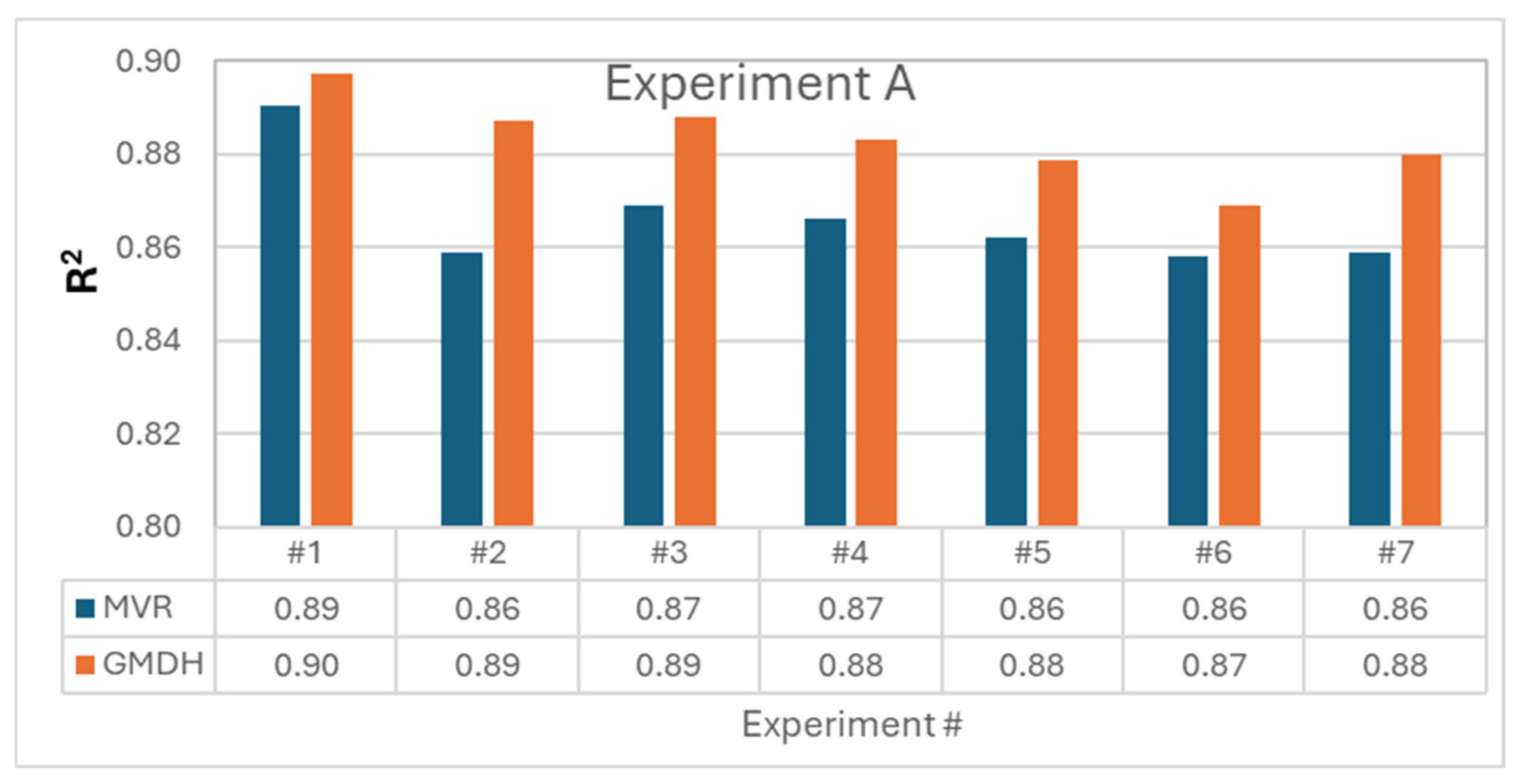The GMDH algorithm, as described in several references [34,35,46,53], utilizes multiple inputs to identify the best combination and generates a quadratic polynomial. An external criterion determines the selection of this optimal combination of two features. Two input features were selected to compare the GMDH method (Equation (8) with MVR (Equation (1)). A total of 18 experiments were designed (Table 3 in Section 3). 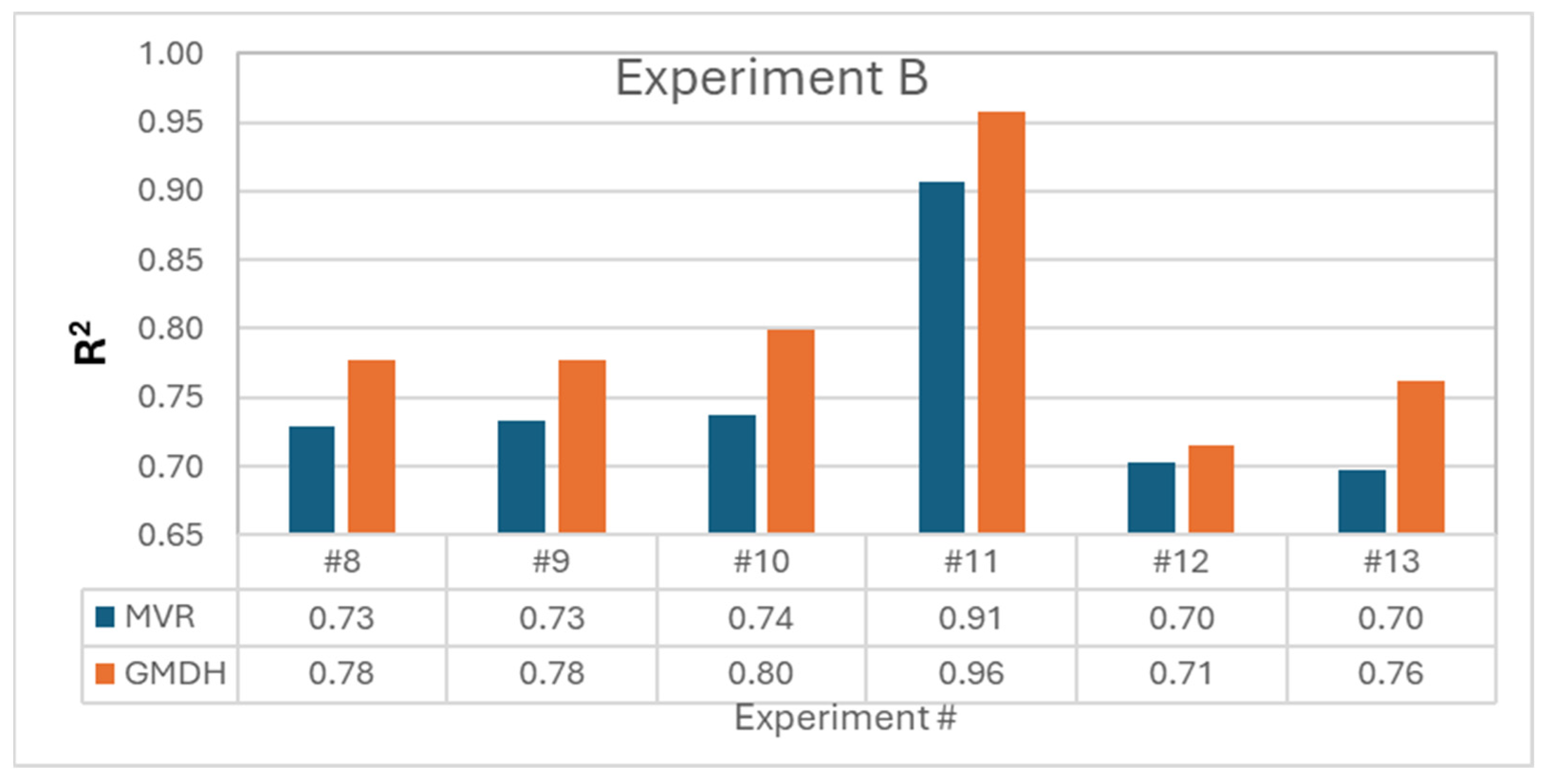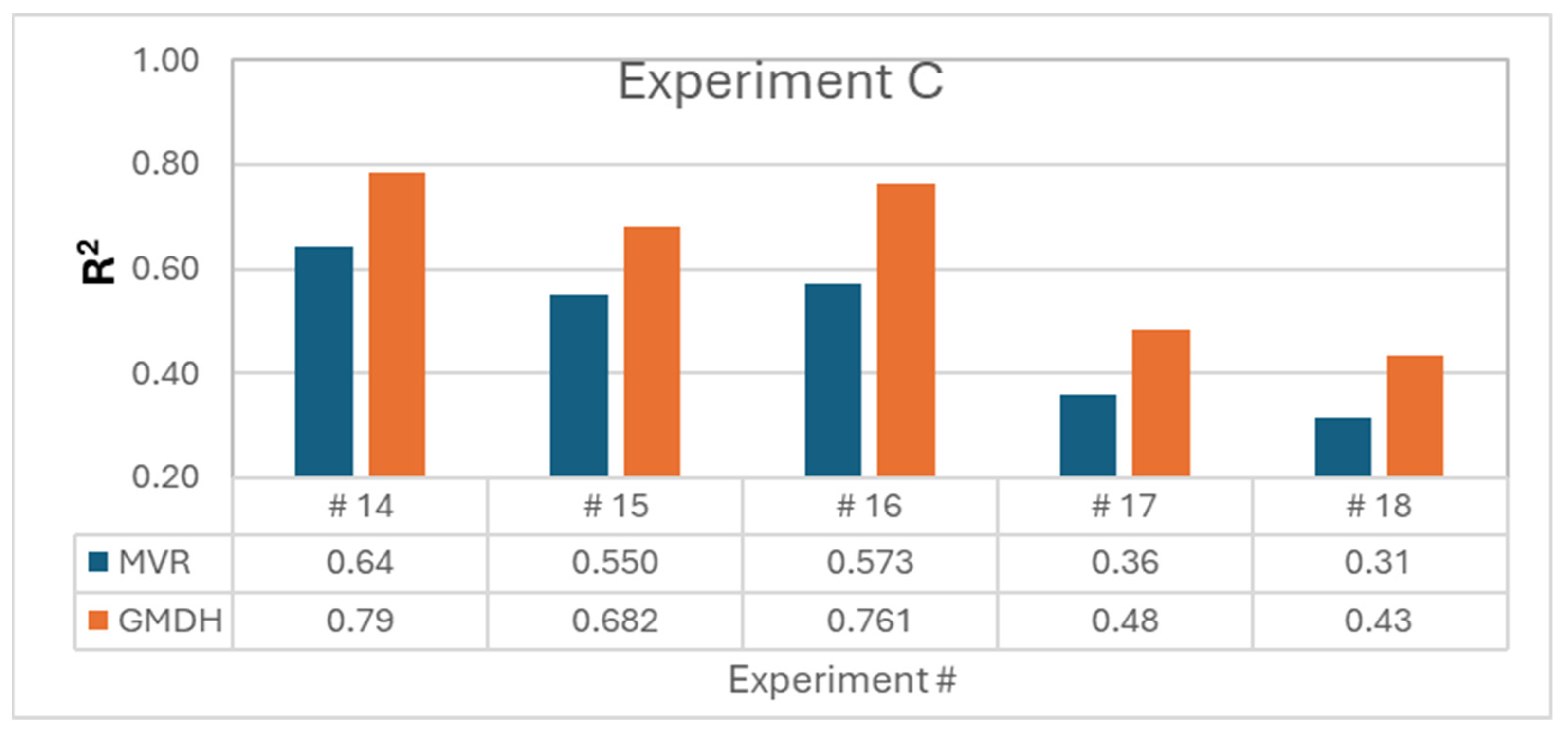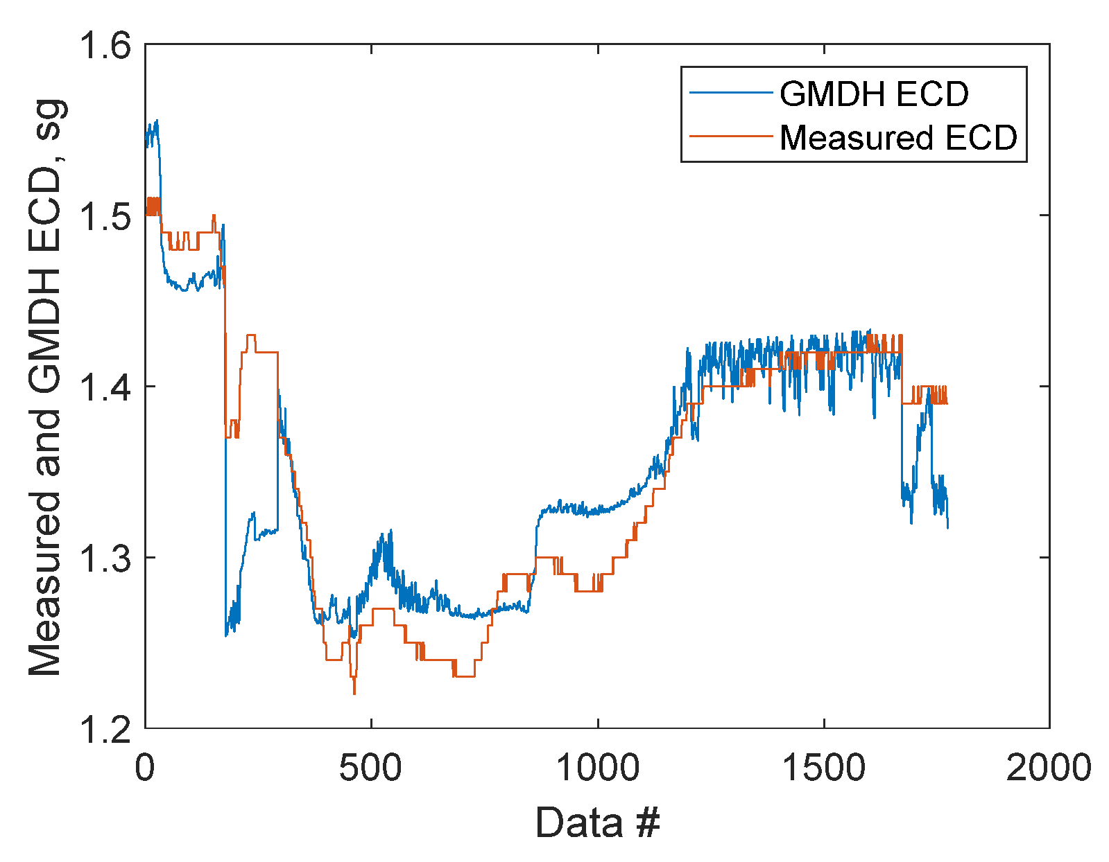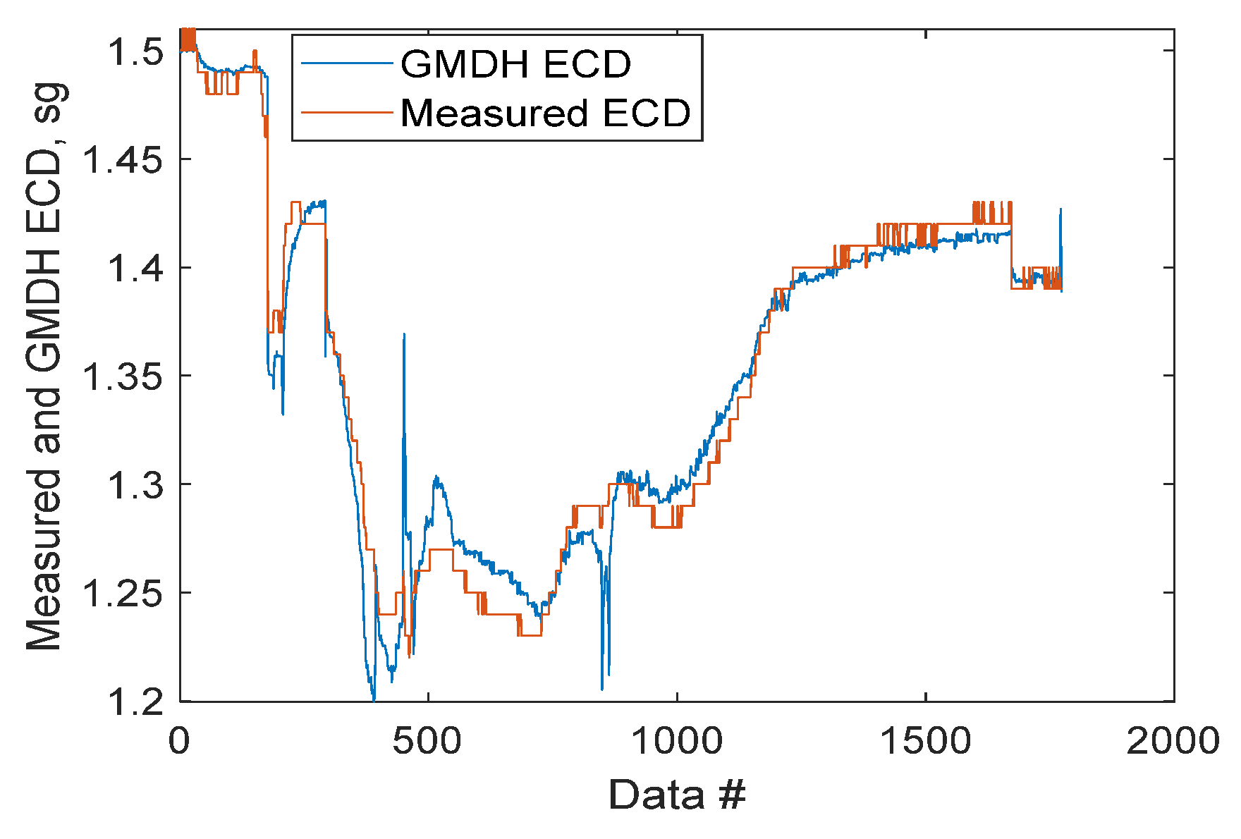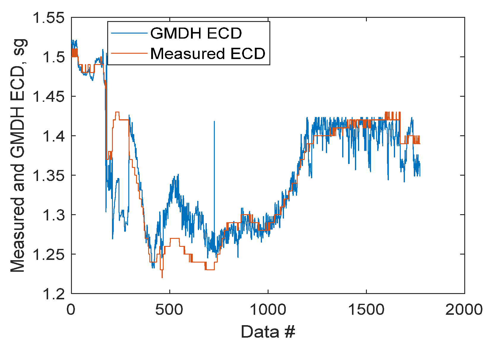Figure 5, Figure 6 and Figure 7 offer a comparison of the results obtained from the experiments. The results showed that all the GMDH models predicted a higher R² compared to the multivariable regression (MVR). This indicated that the nonlinear and interaction terms had a significant effect on the ECD prediction. The degree of the model accuracy performance depended on the correlation of the features with the target variable.

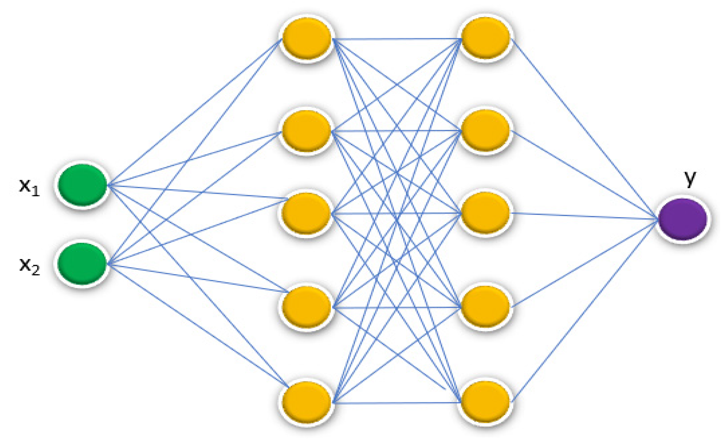
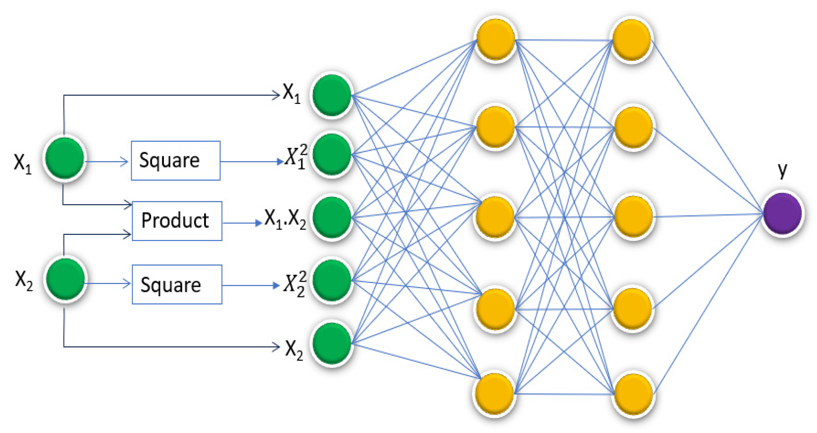
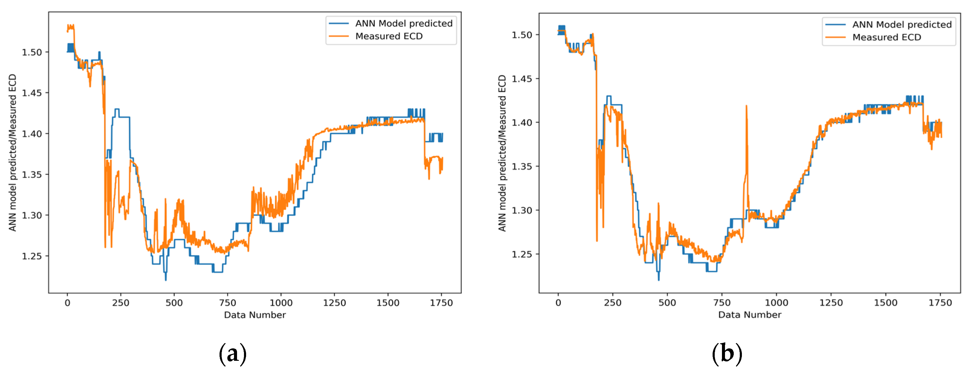
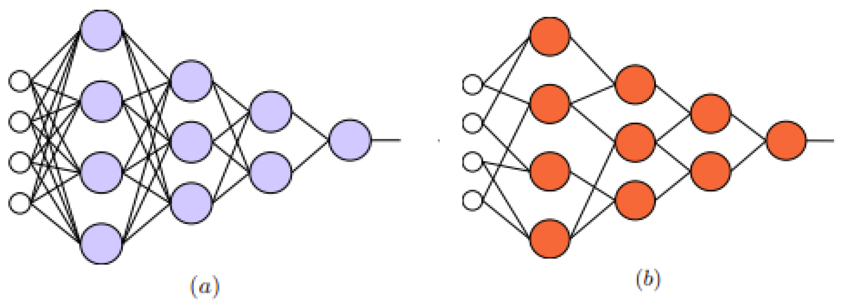
The second part of this study involved comparing the performance of the standard ANN and the proposed GMDH-featured ANN. To ensure consistency in the comparison, both the proposed GMDH-featured ANN (Figure 3) and the fully connected ANN models (Figure 1) were developed, unlike the standard GMDH network where neurons are not fully connected (Figure 2b). The ANN used only two features, and the proposed GMDH-featured ANN had five inputs generated from the two selected features. Out of the eight experimental designs (Table 4), three of the designs showed that the proposed GMDH-featured ANN exhibited a higher model performance as compared with the ANN, whereas the remaining five designs were the same as shown in Table 5. This could have been due to the insignificant impact of the nonlinear and interacting terms.

Table 6. Comparisons of the four ML algorithms results.

Experiment	Output/Input Features		ML Algorithms	R2
	Output	Input
#1	D9	D1  D2	MVR	0.73
		D1  D2	GMDH	0.78
		D1  D2	Normal-featured ANN	0.83
		D1  D2  D1 × D2  (D1)2  (D2)2	GHDH-featured ANN	0.96
#5	D9	D3  D8	MVR	0.55
		D3  D8	GMDH	0.68
		D3  D8	Normal-featured ANN	0.78
		D3  D8  D3 × D8  (D3)2  (D8)2	GHDH-featured ANN	0.87
#8	D9	D4  D5	MVR	0.31
		D4  D5	GMDH	0.43
		D4  D5	Normal-featured ANN	0.69
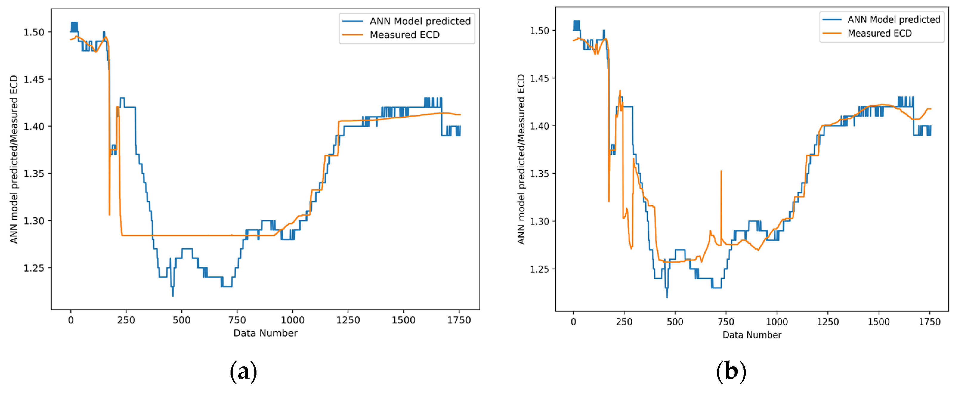
		D4  D5  D4 × D5  (D4)2   (D5)2	GHDH-featured ANN	0.75

displays the input features of the standard ANN and the modeling results obtained from the selected three experiments #1, #5, and #8. Table 5 provides a summary of the model results, showing that the proposed GMDH-featured ANN achieved the R² values of 0.96, 0.87, and 0.75, respectively, compared to the regular ANN with performance accuracies of 0.83, 0.78, and 0.69, respectively. These results indicated that the proposed GMDH-feature ANN had an enhanced performance compared to the regular ANN. However, more experiments need to be performed to examine the model’s performance for other transfer/optimizers and hyperparameters. This will be studied in future work.

Based on the GMDH and MVR, the mathematical model derived from Tests #1, #5, and #8 shown in Table 6 is summarized in

Table 7. Test #1 GMDH and MVR coefficients with input (D1 = pump pressure, and D2 = weight on the bit).

GMDH	xi = D1 and xj = D2	MVR	xi = D1 and xj = D2
Coefficient	Values	Coefficient	Values
a0	1.494609	β0	1.234896
a1	0.001905	β1	0.001227
a2	0.056985	β2	0.007881
a3	0.000009
a4	0.003414
a5	−0.000188
R2	0.78	R2	0.72

,

Table 8. Test #5 GMDH and MVR coefficients with input (D3 = block height, D8 = RPM).

GMDH	xi = D3 and xj = D8	MVR	xi = D3 and xj = D8
Coefficient	10³×	Coefficient	Values
a0	−0.497074	β0	0.958565
a1	0.160636	β1	0.013871
a2	0.010814	β2	0.003009
a3	−0.002787
a4	0.000033
a5	−0.000809
R2	0.68	R2	0.55

and

Table 9. Test #8 GMDH and MVR coefficients with inputs (D4 = bit position and D5 = flow in).

GMDH	xi = D4 and xj = D5	MVR	xi = D4 and xj = D5
Coefficient	10³×	Coefficient	Values
a0	6.812333	β0	19.234220
a1	−0.005875	β1	−0.007818
a2	−0.000025	β2	0.000106
a3	0.0000013
a4	0.0000000002
a5	0.00000001
R2	0.44	R2	0.31

. The GMDH model given in Equation (11) is a function of input data (x_i and x_j) and has six coefficients a₀ to a₅. Similarly, the MVR model shown in Equation (4) has input data (x_i and x_j) with three coefficients β₀ to β₂.

The regression coefficients obtained from the GMDH and MVR were rounded to decimal digits and presented in Table 7, Table 8 and Table 9. Moreover, during MVR modeling, the p-test values of the coefficients of all the experiments showed less than 5%. Hence, the MVR model was statistically significant.

5. Conclusions

The reviewed literature studies indicated that the applications of data-driven modeling have shown satisfactory performance in diverse fields. In this study, a total of four machine learning algorithms were employed to model field drilling datasets and to compare their performances.

Based on the considered modeling setup, the results showed that

➢

the GMDH model exhibited a higher model prediction as compared to the MVR. This could have been due to the impact of the interacting features.

➢

the proposed GMDH-featured ANN model prediction was better than the ANN for about 37.5% of the experiments. For the remaining, both methods’ predictions were the same.

The proposed GMDH-featured ANN model demonstrated exemplary performance based on the considered dataset. However, in future work, additional modeling with diverse datasets will be conducted to evaluate the model performance and limitations. Furthermore, the commonly used fully-unconnected-GMDH-based network will be compared with the proposed methodology.