An Improved Sparrow Search Algorithm for the Optimization of Variational Modal Decomposition Parameters

Abstract

Variational modal decomposition (VMD) is frequently employed for both signal decomposition and extracting features; however, the decomposition outcome is influenced by the quantity of intrinsic modal functions (IMFs) and the specific parameter values of penalty factors. To tackle this issue, we propose an algorithm based on the Halton sequence and the Laplace crossover operator for the sparrow search algorithm–VMD (HLSSA-VMD) to fine-tune the parameters of VMD. First, the population initialization by the Halton sequence yields higher-quality initial solutions, which effectively addresses the issue of the algorithm’s sluggish convergence due to overlapping and the lack of diversity of the initial solutions. Second, the introduction of the Laplace crossover operator (LX) to perturb the position of the best individual in each iteration helps to prevent the algorithm from becoming ensnared in a local optimum and improves the convergence speed of the algorithm. Finally, from the simulation of 17 benchmark test functions, we found that the HLSSA exhibited superior convergence accuracy and accelerated convergence pace, as well as better robustness than the particle swarm optimization (PSO) algorithm, the whale optimization algorithm (WOA), the multiverse optimization (MVO) algorithm, and the traditional sparrow search algorithm (SSA). In addition, we verified the effectiveness of the HLSSA-VMD algorithm on two simulated signals and compared it with PSO-VMD, WOA-VMD, MVO-VMD, and SSA-VMD. The experimental findings indicate that the HLSSA-VMD obtains better parameters, confirming the superiority of the algorithm.

1. Introduction

As science and technology advance swiftly, and with the continuous evolution of social needs, optimization algorithms are becoming increasingly crucial in solving complex problems in various fields. From mechanical design and manufacturing to artificial intelligence, the rapid progress in these fields not only promotes the development of industry but also triggers the demand for optimization algorithms to be more efficient and innovative [1].

Within signal decomposition, numerous techniques have been developed for extracting fault features. Common algorithms include wavelet transform (WT) [2], empirical mode decomposition (EMD) [3], empirical wavelet transform (EWT) [4], and the local mean decomposition (LMD) [5], among others. Although these algorithms are widely applied and play a positive role in many fields, they also exhibit certain issues that impact the effectiveness of signal decomposition. When using WT for signal processing, the fixed choice of mother wavelet leads to a lack of flexibility and less applicability when dealing with different types of signals. EMD suffers from severe mode mixing and endpoint effects when decomposing signals. Although the LMD method efficiently mitigates the emergence of over- and under-envelopes in EMD decomposition, it continues to demonstrate endpoint effects. The limited adaptability and robustness of EWT restrict its capability for signal decomposition.

In 2014, Dragomiretskiy proposed VMD [6], a method with both a strong theoretical basis and notable robustness in extracting fault features in complex environments, such as strong noise. This algorithm has found application across diverse fields and has shown excellent performance [7,8,9]. However, the VMD algorithm itself has limitations, and the effectiveness of its decomposition may be affected by both the quantity of intrinsic mode functions (IMFs), denoted as K, and the parameter α for the penalty factor. With inappropriate parameter settings, issues such as mode mixing may arise when employing the VMD algorithm in signal processing. To address the shortcomings of the VMD algorithm, many researchers opt to employ swarm intelligence optimization algorithms for parameter tuning. Li et al. [10] utilized a genetic algorithm for the adaptive searching of optimal parameters for VMD, while Liu et al. [11] utilized the grey wolf algorithm to acquire the optimal parameters for VMD. Other swarm intelligence algorithms used for optimizing VMD parameters include the PSO [12], WOA [13], multiverse optimization (MVO) algorithm [14], sailfish optimization (SFO) algorithm [15], Archimedes optimization algorithm (AOA) [16], etc.

In 2020, Xue et al. [17] introduced the SSA, known for its computational efficiency, simplicity of implementation, and ease of scalability. According to Xue et al.’s analysis, the SSA demonstrates superior performance compared to several established algorithms like the PSO, GWO, and gravity search algorithm (GSA) regarding convergence accuracy, convergence speed, and robustness. Nevertheless, akin to other swarm intelligence algorithms, the SSA may suffer from low initial solution quality, and in solving complex optimization problems, it may experience a decrease in population diversity and vulnerability to becoming trapped in local optima toward the later stages of the solution process. Researchers have addressed the aforementioned issues and achieved positive results through various studies. Gao et al. [18] proposed a multistrategy enhanced evolutionary sparrow search algorithm (ESSA), integrating tent map chaos during the initialization phase to expedite convergence speed and improve convergence accuracy. Geng et al. [19] introduced chaotic back-propagation learning and dynamic weights to prevent the SSA from being entrapped in local optima. Wu et al. [20] combined Levy flights and nonlinear inertia weight to present an improved SSA. Xiong et al. [21] introduced a fractional-order chaotic improved SSA, demonstrating higher convergence accuracy than the SSA. Sun et al. [22] implemented CAT chaotic mapping to initialize a population and explored the initial population’s randomness and searchability. Han et al. [23] used sin chaotic mapping to initialize the sparrow population, aiming to improve the quality of initial solutions. Liu et al. [24] introduced circular chaotic mapping into the SSA, enhancing the algorithm’s capacity for global exploration during population initialization. They additionally introduced the t-distribution in the formula for updating the positions of sparrows across various iteration cycles, aiding the algorithm in avoiding local optima.

The current research places significant emphasis on the population initialization process in the SSA since the population’s quality distribution significantly influences the efficacy of the search for the global optimum. In the early stages of the algorithm, a well-designed population initialization process can effectively improve the algorithm’s capability for global exploration. Chaos mapping is a frequently used approach in the existing literature on initialization, as mentioned above. However, chaotic systems are highly sensitive to starting conditions and display unpredictable randomness. Additionally, chaotic mapping algorithms involve complex mathematical operations, leading to increased computational costs.

In this paper, we propose the Halton sequence for population initialization. In comparison to the aforementioned methods, the Halton sequence ensures a more uniformly distributed initial population across the entire space and lacks random components, making it more robust. Moreover, its lower sensitivity to initial conditions and parameters enhances its reliability in algorithm applications. The crossover operator plays a crucial role in optimization algorithms by promoting population diversity and exploring the search space. The Laplace crossover operator (LX) is a particularly unique crossover operator that has been applied in various fields [25,26]. Deep et al. [27] first introduced the LX in 2007 and applied it to genetic algorithms (GAs). Experimental results demonstrated that the LX-GA outperformed other types of GAs. Consequently, in many studies related to GAs, researchers tend to utilize the LX for performing crossover operations [28,29]. The LX is suitable for optimization problems involving continuous parameters and generates random numbers based on the Laplace distribution, exhibiting good randomness and perturbation properties. Additionally, the basic operation of the LX is based on the Laplace distribution, requiring minimal parameter tuning. Considering the numerous advantages of the LX, in this study, we utilized the LX to disturb the position of the best individual at each iteration with the goal of improving the algorithm’s ability for local exploration and preventing the population from becoming ensnared in local optima. The primary contributions of this paper are outlined as follows:

(1)

In the sparrow initialization stage, cleverly utilizing the Halton sequence to generate initial solutions effectively improves the quality of the initial solutions, thereby significantly enhancing the algorithm’s robustness. This initialization strategy not only aids in a more evenly distributed set of initial solutions across the entire solution space but also reduces the algorithm’s sensitivity to initial conditions.

(2)

Introducing the Laplace crossover operator to cleverly perturb the position of the best individual in each iteration successfully mitigates the possibility of the algorithm becoming ensnared in local optima while significantly improving the convergence speed. By incorporating this effective local search strategy during the optimization process, we effectively expanded the algorithm’s exploration range in the solution space.

(3)

We extensively validated the effectiveness and outstanding performance of the algorithm on 17 benchmark functions. Moreover, the enhanced algorithm was effectively employed in optimizing parameters for the VMD algorithm, ultimately achieving satisfactory results and thus highlighting the practical value of this algorithm.

The remainder of the paper is organized as follows: Section 2 outlines the pertinent theoretical approaches contributing to our understanding. Section 3 provides a comprehensive description of the method proposed in this paper. Section 4 validates the proposed methodology. Finally, Section 5 presents the conclusions of this study, along with suggestions for future work.

2. The Principles of SSA

In the SSA, a population consisting of n sparrows can be represented in the following form:

$$X=\left[\begin{array}{cccc}{x}_{1,1}& x_{1,2}& \cdots & x_{1,d}\\ x_{2,1}& x_{2,2}& \cdots & x_{2,d}\\ ⋮& ⋮& ⋮& ⋮\\ x_{n,1}& x_{n,2}& \cdots & x_{n,d}\end{array}\right]$$

(1)

where d represents the dimensionality of the problem to be solved. The fitness values of all sparrows can be represented in the following form:

$$F_X=\left[\begin{array}{c}f([x_{1,1} x_{1,2} \cdots x_{1,d}])\\ f([x_{2,1} x_{2,2} \cdots x_{2,d}])\\ ⋮\\ ⋮\\ f([x_{n,1} x_{n,2} \cdots x_{n,d}])\end{array}\right]$$

(2)

where f represents an individual’s fitness value, and $F_X$ represents the fitness value of all sparrows.

The primary task of the founder in the sparrow population is to search for food in the environment, providing the entire population with the location and direction of the discovered food. Since founders are more likely to find food, the fitness values of producers are superior, and their position in the entire solution space is close to the location of the optimal solution. During each iteration of the search process, the founder updates its position while searching for food, and the specific calculation is expressed with the following equation:

$$X_{i,j}^{t+1}=\left\{\begin{array}{l}{X}_{i,j}^t\cdot \exp (-\frac{i}{\alpha \cdot ite{r}_{\max }}) if R_2<ST\\ X_{i,j}^t+Q\cdot Lif R_2\ge ST\end{array}\right.$$

(3)

where t denotes the current iteration number; j = 1, 2, 3, ..., d; $ite{r}_{\max }$ represents the current maximum iteration count; $X_{ij}$ represents the position of the i-th sparrow along the j-th dimension; and $\alpha \in (0,1)$ is the uniform random number. $R_2$($R_2\in \left[0,1\right]$) and ST ($ST\in \left[0.5,1\right]$) denote the warning value and safety value, respectively. Q is a randomly generated number following a normal distribution, and L represents a $1\times d$ matrix, where every element in the matrix is equal to 1.

$R_2<ST$ indicates that, in the foraging environment, there are no predators present, allowing the founder to explore freely and extensively. However, $R_2\ge ST$ indicates that certain sparrows within the population have detected predators and signaled warnings to other members. Consequently, all sparrows must promptly relocate to alternative safe locations for foraging.

While foraging, certain scroungers consistently observe the founder. Upon realizing that the founder has discovered superior food, they promptly abandon their current position to vie for the food. The position update process for scroungers is outlined as follows:

$$X_{i,j}^{t+1}=\left\{\begin{array}{l}Q\cdot \exp (\frac{X_{worst}-X_{i,j}^t}{i^2})if i>n/2\\ X_P^{t+1}+\left|X_{i,j}^t-X_P^{t+1}\right|\cdot A^{+}\cdot L otherwise\end{array}\right.$$

(4)

where $X_P$ represents the current optimal position held by the founder; $X_{worst}$ represents the current globally worst position; A is a $1\times d$ matrix consisting of elements randomly assigned values of either 1 or −1; and $A^{+}=A^T{(A{A}^T)}^{-1}$. When $i>n/2$, the i-th joiner with a lower fitness value has not yet secured food and is in a highly hungry state. Consequently, it must relocate to another area for foraging to replenish its energy.

In the simulation experiments, the proportion of sparrows exhibiting danger perception was determined to range between 10% and 20% of the total population. Their initial positions are randomly distributed throughout the entire population, and their mathematical representation is as follows:

$$X_{i,j}^{t+1}=\left\{\begin{array}{l}{X}_{best}^t+\beta \cdot \left|X_{i,j}^t-X_{best}^t\right| if f_i>f_g\\ X_{i,j}^t+K\cdot (\frac{\left|X_{i,j}^t-X_{worst}^t\right|}{(f_i-f_w)+\epsilon }) if f_i=f_g\end{array}\right.$$

(5)

where $X_{best}$ represents the present global optimal position; $\beta$ represents the step size control parameter, with its value being a randomly generated number following a normal distribution with a mean of 0 and a variance of 1; $K\in (-1,1)$ is the uniform random number; $f_i$ is the fitness score of the present sparrow individual; $f_g$ and $f_w$ represent the current global best and worst fitness values, respectively; and $\epsilon$ is a numerically small constant to prevent division by zero. When $f_i>f_g$, the sparrow is at the population boundary and susceptible to predator attacks, signifying that the sparrow’s position is the safest at this point. When $f_i=f_g$, sparrows in the centroid of the population have detected danger, so they need to converge with other sparrows to minimize the threat of predation.

3. Improved SSA Based on Halton Sequence and LX

3.1. Population Initialization Based on the Halton Sequence

The Halton sequence [30,31,32] is a common multidimensional low-discrepancy sequence with an optimal order difference of $N^{-1}{\left(\log \left(N\right)\right)}^d$, where d is the dimension. As shown in Figure 1, the solutions generated with the Halton sequence are more uniformly distributed in space than those generated using random initialization.

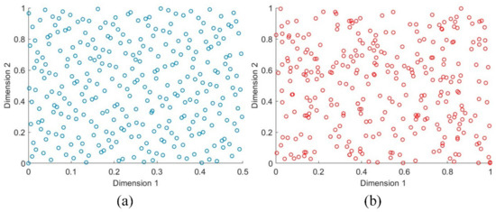
Figure 1. (a) Halton sequence initialization; (b) random sequence initialization.

The definition of the Halton sequence is based on the inverse radical function, and its defining function is expressed as follows:

$${\varphi }_p(n)=\frac{b_0}{p}+\frac{b_1}{p^2}+\cdots +\frac{b_m}{p^{m+1}}$$

(6)

where p is a prime number, and $b_k$ is the k-th digit of n in the base-b expansion ($0\le k\le m$).

$$n=b_0+b_{1}p+\cdots +b_m{p}^m$$

(7)

The Halton sequence in d dimensions can be represented with the following formula:

$$HaltonSe{t}_n=\left({\varphi }_{p_1}\left(n\right),{\varphi }_{p_2}\left(n\right),\cdots ,{\varphi }_{p_d}\left(n\right)\right)$$

(8)

The initial positions for the population can be generated using the following formula:

$$x_{i,j}=l{b}_j+HaltonSe{t}_n\times \left(u{b}_j-l{b}_j\right)$$

(9)

where $l{b}_j$ and $u{b}_j$ denote the lower and upper limits of the positions of the sparrow population in the j-th dimension ($1\le i\le n,1\le j\le d$).

3.2. Optimal Position Perturbation Based on LX

The LX generates a pair of offspring, $y_1=\left(y_1^1,y_1^2,\cdots ,y_1^a\right)$ and $y_2=\left(y_2^1,y_2^2,\cdots ,y_2^a\right)$, from a pair of parents, namely $x_1=\left(x_1^1,x_1^2,\cdots ,x_1^a\right)$ and $x_2=\left(x_2^1,x_2^2,\cdots ,x_2^a\right)$. The descendants produced by the LX are symmetrically positioned relative to the parents. LX random numbers are determined according to the following rules [27]:

$$l_s=\left\{\begin{array}{l}p-q{\log }_e\left(u_s\right) v_s\le 1/2\\ p+q{\log }_e\left(u_s\right) v_s>1/2\end{array}\right.$$

(10)

where $u_s$ and $v_s$ are two random numbers uniformly distributed within the range [0, 1]; $p\in R$ is the location parameter, which can be used to control the distribution of the offspring positions in the search space; and $q>0$ is the scale parameter. A smaller q value results in offspring positions being closer to the parents, while a larger q value leads to offspring positions being farther from the parents. In this study, the value of q was 1, and the value of p was 0. The rules for offspring generation are as follows:

$$\begin{array}{l}{y}_1^s=x_1^s+l_s\left|x_1^s-x_2^s\right|\\ y_2^s=x_2^s+l_s\left|x_1^s-x_2^s\right|\end{array}$$

(11)

If the range of offspring positions exceeds the search space, i.e., $y_j<l{b}_j$ or $y_j>u{b}_j$, then $y_j$ is set to a random number from the interval $\left[l{b}_j,u{b}_j\right]$.

The pseudocode of HLSSA is shown in Algorithm 1.

Algorithm 1 Pseudocode of HLSSA

1. set t = 0

2. Initialize the population using Equation (9).

3. compute the fitness value for each sparrow individual using the fitness function, and then arrange them in order, noting the best position $X_{best}$ and best fitness value $f_g$.

4. While (t < $ite{r}_{\max }$)

determine the proportion of founders PD1, the ratio of scroungers PD2 and the proportion of sparrows with danger perception PD3

For i = 1: PD1

Update the founders positions based on Formula (3).

End for

For i = 1: PD2

Update the scroungers positions based on Formula (4).

End for

For i = 1: PD3

Update the sparrows with danger perception positions based on Formula (5).

End for

Calculate the fitness value for each sparrow and select the best one.

Disturb the optimal position according to Formula (11) and compute its fitness value. Compare the fitness values before and after the disturbance and choose the better one.

t = t + 1

End while

5. Return $X_{best}$,$f_g$

4. Method Validation

To assess the effectiveness of the enhanced algorithm, two sets of comparative experiments were devised in this study. In the initial set of experiments, we selected seven unimodal test functions, characterized by having only one extremum, to verify the algorithm’s convergence speed, optimization accuracy, and local search capability. The second set of experiments involved the selection of five multimodal test functions, characterized by having multiple local extremum points, to examine the algorithm’s performance in escaping local optima and possessing global exploration capabilities. To reduce the bias in single-run results, we conducted 30 iterations for each function and documented their optimal values, mean values, and standard deviations. Simultaneously, we compared the improved algorithm with the PSO, MVO, WOA, and SSA. Table 1 provides the detailed parameter settings of each algorithm. All experiments were executed on a computer featuring an Intel i7 processor operating at 2.30 GHz and 16 GB of RAM, utilizing the MATLAB 2023a environment. This experimental design and environment setup aimed to comprehensively and reliably evaluate algorithm performance and facilitate an objective comparison.

Table 1. Details of algorithm parameter settings.

Algorithm	Parameters
PSO	Particle count: 30; max iterations: 500; learning factors: c1 = c2 = 1.5; inertia weight: w = 0.7;
MVO	number of universes: 30; maximum iteration count: 500; probability for the existence of wormholes: $WEP\in \left[0.2,1\right]$
WOA	Number of whales: 30; maximum iteration count: 500;
SSA	population size: 30; maximum iteration count: 500; warning value: ST = 0.6; the proportion of founders: PD = 0.7, the rest are joiners; the ratio of sparrows aware of the presence of sparrows that sense danger and sound the alarm: SD = 0.2
HLSSA	Population size: 30; maximum iteration count: 500; warning value: ST = 0.6; the proportion of founders: PD = 0.7, the rest are joiners; the ratio of sparrows of the presence of sparrows that sense danger and sound the alarm: SD = 0.2; Halton sequence parameters: Skip = 0, Leap = 1; LX parameters: p = 0.5, q = 1

4.1. Unimodal Test Function Experiments

Evaluating algorithm performance using test functions with known global optimal values is a common approach in this field. Unimodal test functions are particularly useful for validating algorithm performance in local search, as these functions contain only one global optimum without other local optima. Table 2 provides the formulas, dimensions, search space, and global optimal values for unimodal test functions. The optimal value represents the global minimum value, and the search space refers to the range of $x_i$.

Table 2. Details of unimodal benchmark functions.

Benchmark Functions	n (Dimension)	Search Space	Optimal Value
$F_1(x)={\displaystyle \sum _{i=1}^n{x}_i^2}$	30	[−100, 100]	0
$F_2(x)={\displaystyle \sum _{i=1}^n\left|x_i\right|}+{\displaystyle \prod _{i=1}^n\left|x_i\right|}$	30	[−10, 10]	0
$F_3(x)={{\displaystyle {\sum }_{i=1}^n({\displaystyle {\sum }_{j=1}^i{x}_j})}}^2$	30	[−100, 100]	0
$F_4(x)={\max }_i\left\{\left|x_i\right|,1\le i\le n\right\}$	30	[−100, 100]	0
$F_5(x)={\displaystyle {\sum }_{i=1}^{n-1}\left[100{\left(x_{i+1}-x_i^2\right)}^2+{\left(x_i-1\right)}^2\right]}$	30	[−30, 30]	0
$F_6(x)={{\displaystyle {\sum }_{i=1}^n\left(\left[x_i+0.5\right]\right)}}^2$	30	[−100, 100]	0
$F_7(x)={\displaystyle {\sum }_{i=1}^{n}i{x}_i^4}+random\left[0,1\right)$	30	[−1.28, 1.28]	0

4.1.1. Experimental Results

Table 3 presents the optimization outcomes for the five algorithms; the “Best” column lists the best fitness values. Figure 2, Figure 3, Figure 4, Figure 5, Figure 6, Figure 7 and Figure 8 present three-dimensional plots and convergence curves for the seven benchmark functions. In Figure 2a, Figure 3a, Figure 4a, Figure 5a, Figure 6a, Figure 7a and Figure 8a, n = 2 for the purpose of displaying the two-dimensional surface of the functions. In the results shown in Figure 2b, Figure 3b, Figure 4b, Figure 5b, Figure 6b, Figure 7b and Figure 8b, the value of n is 30.

Table 3. Results of optimizing seven unimodal benchmark functions using the five algorithms.

Function	Algorithm	Best	Average	STD	Variance
F1	PSO	0.00033	0.002926391	0.00251	6.302 × 10−6
	MVO	0.0060158	0.013780395	0.006517521	4.24781 × 10−5
	WOA	1.88 × 10−85	1.47 × 10−74	2.98625 × 10−74	8.9177 × 10−148
	SSA	0	5.54 × 10−86	1.9214×10−85	3.6918 × 10−170
	HLSSA	0	0	0	0
F2	PSO	0	0	0	0
	MVO	0.016637	0.03681265	0.011406764	0.000130114
	WOA	9.31 × 10−57	4.58 × 10−51	1.31735 × 10−50	1.7354 × 10−100
	SSA	0	1.26 × 10−45	3.79338 × 10−45	1.43898 × 10−89
	HLSSA	0	0	0	0
F3	PSO	0.01202	0.12741265	0.1465195	0.021467964
	MVO	0.010296	0.12150025	0.089212352	0.007958844
	WOA	1.51	4.33 × 104	12,839.5126	164,853,083.9
	SSA	0	1.89 × 10−62	8.23118 × 10−62	6.7752 × 10−123
	HLSSA	0	0	0	0
F4	PSO	0.01247	0.18308305	0.124116834	0.015404989
	MVO	0.042594	0.09646565	0.035631193	0.001269582
	WOA	0.132006517	36.21277267	30.75549409	945.9004169
	SSA	0	2.10 × 10−48	8.89079 × 10−48	7.90461 × 10−95
	HLSSA	0	0	0	0
F5	PSO	6.3088	33.794385	41.36261671	1710.866061
	MVO	6.8941	137.409115	203.9184648	41,582.74029
	WOA	27.05372992	27.97991864	0.501056388	0.251057504
	SSA	9.40 × 10−8	6.21 × 10−5	9.98646 × 10−5	9.97294 × 10−9
	HLSSA	2.75 × 10−9	1.75 × 10−6	2.57505 × 10−6	6.63087 × 10−12
F6	PSO	0.00020952	0.00419352	0.004367111	1.90717 × 10−5
	MVO	0.0037676	0.01302205	0.005310819	2.82048 × 10-5
	WOA	0.141565425	0.423901093	0.233104106	0.054337524
	SSA	6.86 × 10−10	2.96 × 10−7	3.99442 × 10−7	1.59554 × 10−13
	HLSSA	2.67 × 10−13	3.25 × 10−9	2.99447 × 10−9	8.96684 × 10−18
F7	PSO	0.00015349	0.000624792	0.000462511	2.13917 × 10−7
	MVO	0.0013722	0.003321475	0.001558795	2.42984 × 10−6
	WOA	3.21249 × 10−5	0.005392808	0.005106315	2.60745 × 10−5
	SSA	0.000066649	0.000400385	0.000294376	8.66569 × 10−8
	HLSSA	2.09 × 10−6	4.91 × 10−5	2.81604 × 10−5	7.93008 × 10−10

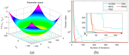
Figure 2. (a) Three-dimensional plot of F₁; (b) convergence curve.

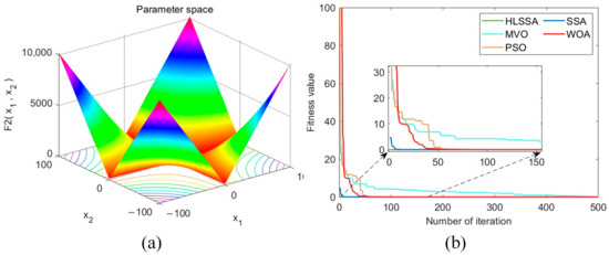
Figure 3. (a) Three-dimensional plot of F₂; (b) convergence curve.

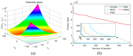
Figure 4. (a) Three-dimensional plot of F₃; (b) convergence curve.

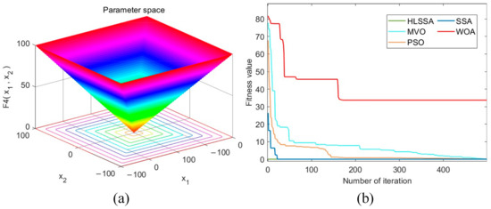
Figure 5. (a) Three-dimensional plot of F₄; (b) convergence curve.

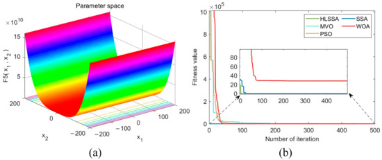
Figure 6. (a) Three-dimensional plot of F₅; (b) convergence curve.

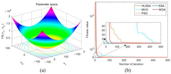
Figure 7. (a) Three-dimensional plot of F₆; (b) convergence curve.

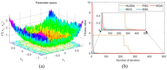
Figure 8. (a) Three-dimensional plot of F₇; (b) convergence curve.

4.1.2. Analysis of the Results

Convergence accuracy analysis: As depicted in Table 3, using the HLSSA, we successfully determined the optimal values for test functions F₁ to F₄. Although they did not reach the optimal values for F₅ to F₇, the algorithm’s performance in terms of the obtained optimal values, averages, and standard deviations was significantly better than the PSO, MVO, WOA, and SSA. This indicates that the HLSSA has stronger optimization capabilities when solving unimodal test functions.

Stability analysis: According to the standard deviation (STD) test data in Table 3, the HLSSA had STD values of 0 for F₁ to F₄ and the lowest STD values for F₅ to F₇. This suggests that the HLSSA has better stability on unimodal test functions than other algorithms.

Convergence speed analysis: As shown in Figure 2, Figure 3, Figure 4, Figure 5, Figure 6, Figure 7 and Figure 8, the HLSSA had an absolute advantage in convergence speed on test functions F₁ to F₇. On test functions F₁ to F₄ and F₆, HLSSA yielded the optimal values at the beginning of the iterations, indicating that initialization based on the Halton sequence helps the algorithm obtain better initial solutions.

In summary, the proposed HLSSA exhibited stronger optimization capabilities, faster convergence speed, and greater stability when dealing with unimodal functions. This study proposes an efficient and reliable algorithm for unimodal test function optimization problems.

4.2. Multimodal Test Function Experiments

Multimodal test functions typically contain many local optimum values, making them more challenging and difficult to use for finding the global optimum. Therefore, testing on such functions allows for a more comprehensive evaluation of the algorithm’s exploration capabilities and potential to escape local optima. Table 4 provides the formulas, dimensions, search spaces, and global optimal values for multimodal test functions.

Table 4. Details of multimodal benchmark functions.

Benchmark Functions	n (Dimension)	Search Space	Optimal Value
$F_8(x)={\displaystyle {\sum }_{i=1}^n-x_i\sin \left(\sqrt{\left|x_i\right|}\right)}$	30	[−500, 500]	−12,569.5
$F_9(x)={\displaystyle {\sum }_{i=1}^n\left[x_i^2-10\cos (2\pi x_i)+10\right]}$	30	[−5.12, 5.12]	0
$\begin{array}{l}{F}_{10}(x)=-20\exp (-0.2\sqrt{\frac{1}{n}{\displaystyle \sum _{i=1}^n{x}_i^2}})-\\ \exp (\frac{1}{n}{\displaystyle \sum _{i=1}^n\cos (2\pi x_i)})+20+e\end{array}$	30	[−32, 32]	0
$F_{11}(x)=\frac{1}{4000}{\displaystyle \sum _{i=1}^n{x}_i^2-{\displaystyle \prod _{i=1}^n\cos (\frac{x_i}{\sqrt{i}})}}+1$	30	[−600, 600]	0
$\begin{array}{l}{F}_{12}(x)=\frac{\pi }{n}\{10\sin (\pi y_1)+{\displaystyle \sum _{i=1}^{n-1}{(y_i-1)}^2}[1+10{\sin }^2(\pi y_{i+1})+\\ (y_n-1{)}^2]\}+{\displaystyle \sum _{i=1}^{n}u(x_i,10,100,4),y_i=1+\frac{x_i+1}{4}},\\ u(x_i,a,k,m)=\left\{\begin{array}{l}k(x_i-a{)}^m,x_i>a\\ 0,-a<x_i<a\\ k(-x_i-a{)}^m, x_i<-a\end{array}\right.\end{array}$	30	[−30, 30]	0

4.2.1. Experimental Results

Table 5 presents the optimization results for the five algorithms, and Figure 9, Figure 10, Figure 11, Figure 12 and Figure 13 depict the three-dimensional plots and convergence plots for the five test functions. In Figure 9a, Figure 10a, Figure 11a, Figure 12a and Figure 13a, n = 2 for the purpose of displaying the two-dimensional surface of the functions. In the results shown in Figure 9b, Figure 10b, Figure 11b, Figure 12b and Figure 13b, the value of n is 30.

Table 5. Optimization results of the five algorithms on five unimodal benchmark functions.

Function	Algorithm	Best	Average	STD	Variance
F8	PSO	−1880.0986	−2524.558865	377.4638744	142,478.9765
	MVO	−2154.8354	−3008.179335	380.7394914	144,962.5603
	WOA	−1.26 × 104	−1.03 × 104	1727.512209	2,984,298.431
	SSA	−12,569.0584	−10,417.30763	2201.824506	4,848,031.157
	HLSSA	−12,569.5	−12,569.5	1.81899 × 10−12	3.30872 × 10−24
F9	PSO	6.0018	23.206275	14.66438476	215.0441805
	MVO	6.9718	15.52885	5.804935452	33.6972756
	WOA	0	0	0	0
	SSA	0	0	0	0
	HLSSA	0	0	0	0
F10	PSO	0.015674	1.260136	0.819697672	0.671904273
	MVO	0.028273	0.20785755	0.48086254	0.231228782
	WOA	4.44 × 10−16	4.53 × 10−15	2.58031 × 10−15	6.65799 × 10−30
	SSA	4.44 × 10−16	4.44 × 10−16	9.86076 × 10−32	9.72346 × 10−63
	HLSSA	4.44 × 10−16	4.44 × 10−16	9.86076 × 10−32	9.36772 × 10−33
F11	PSO	0.024742	0.12481485	0.068084759	0.004635534
	MVO	0.17882	0.312224	0.124271598	0.01544343
	WOA	0	0.02551	0.07007949	0.004911135
	SSA	0	0	0	0
	HLSSA	0	0	0	0
F12	PSO	0.00068858	0.126635751	0.326288108	0.10646393
	MVO	0.00029349	0.107082826	0.28195128	0.079496524
	WOA	0.0052	0.021755	0.022362323	0.000500073
	SSA	1.14 × 10−10	7.83 × 10−8	1.24041 × 10−7	1.53862 × 10−14
	HLSSA	1.44 × 10−13	2.57 × 10−9	2.7137 × 10−9	7.36418 × 10−18

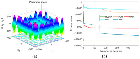
Figure 9. (a) Three-dimensional plot of F₈; (b) convergence curve.

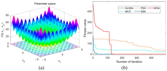
Figure 10. (a) Three-dimensional plot of F₉; (b) convergence curve.

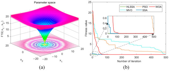
Figure 11. (a) Three-dimensional plot of F₁₀; (b) convergence curve.

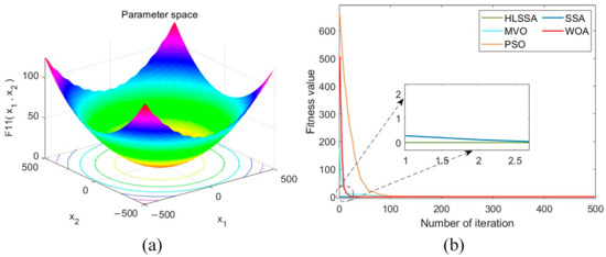
Figure 12. (a) Three-dimensional plot of F₁₁; (b) convergence curve.

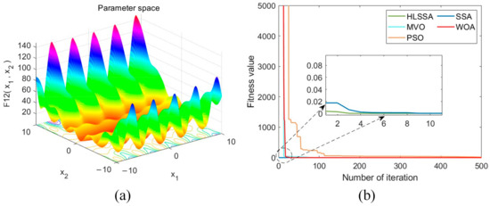
Figure 13. (a) Three-dimensional plot of F₁₂; (b) convergence curve.

4.2.2. Analysis of the Results

Convergence accuracy analysis: As shown in Table 5, the HLSSA successfully yielded the optimal values for test functions F₈, F₉, and F₁₁, and its optimization performance was significantly better than the PSO, MVO, and WOA. Although the HLSSA did not yield the optimal values for F₁₀ and F₁₂, its performance in terms of the obtained optimal values, averages, and standard deviations was still better than other algorithms. For F₉, F₁₀, and F₁₁, the SSA performed similarly to the HLSSA, but regarding the other two functions, the SSA was more prone to becoming entrapped in local optima. Overall, the HLSSA exhibited stronger global search capabilities when solving multimodal test functions, confirming the effectiveness of LX perturbation in helping the SSA escape local optima.

Stability analysis: According to the standard deviation (STD) data in Table 5, the HLSSA exhibited comparable performance to the SSA considering F₉, F₁₀, and F₁₁. However, in terms of the remaining multimodal test functions, the HLSSA revealed consistently lower STD values, indicating better stability on multimodal test functions.

Convergence speed analysis: As shown in Figure 9, Figure 10, Figure 11, Figure 12 and Figure 13, the HLSSA had an absolute advantage in convergence speed on the five multimodal test functions, and the initial solutions obtained were very close to the optimal values. This suggests that the HLSSA demonstrates accelerated convergence when addressing high-dimensional complex problems.

In summary, the HLSSA exhibited enhanced convergence accuracy, accelerated convergence speed, and improved stability when dealing with high-dimensional multimodal problems. Compared to the basic SSA, the HLSSA achieved significant improvements in performance.

4.3. HLSSA-VMD Algorithm Validation

Variational mode decomposition (VMD) is one of the most commonly used methods in the field of signal decomposition, and its decomposition performance is often heavily influenced by the number of modes (K) and the quadratic penalty term (α). Improper parameter settings can lead to information loss and frequency aliasing. Researchers typically employ optimization algorithms for parameter tuning, yet different optimization algorithms yield varying degrees of effectiveness in optimization. This section presents two sets of simulated signals for validating the effectiveness of the HLSSA-VMD algorithm. A comparative analysis was conducted with the PSO-VMD, WOA-VMD, MVO-VMD, and SSA-VMD to further highlight the superior performance of the HLSSA-VMD algorithm.

The first set of simulated signals we constructed is the simulated signal representing an outer race fault in a bearing, denoted as x(t). The construction formula is as follows [33]:

$$\left\{\begin{array}{l}x(t)=x_1(t)+x_2(t)+x_3(t)+n(t)\\ x_1(t)=A{e}^{-\xi 2\pi f_{n}t}\sin (2\pi f_n\sqrt{1-{\xi }^{2}t})\\ x_2(t)={\displaystyle \sum _{i=1}^M{l}_i\sin (2\pi f_i^{1}t+{\theta }_i)}\\ x_3(t)={\displaystyle \sum _{i=1}^N{k}_i\sin (2\pi f_i^{2}t+{\phi }_i)}\end{array}\right.$$

(12)

where $f_n$ is the natural frequency; $\xi$ is the damping coefficient; A is the amplitude of the pulse fault; and n(t) is Gaussian white noise with an SNR of −10 dB.

The detailed information of the simulated signal is shown in Table 6, with a sampling frequency of 20 KHz and a number of 4096 data samples. Figure 14a,b display the initial state and the state after adding Gaussian white noise to the simulated bearing fault signal, respectively.

Table 6. The detailed parameters of the simulated signal.

Signal	Parameters
$x_1(t)$	A	$\xi$	$f_n$ (Hz)
	3	0.02	2600
$x_2(t)$	M	l	$f_1^1$ (Hz)	${\theta }_1$
	1	0.025	70	0
$x_3(t)$	N	k	$f_1^2$ (Hz)	${\phi }_1$
	1	0.035	100	0

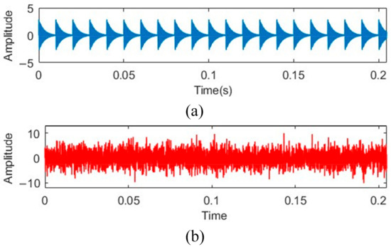
Figure 14. Two states of the bearing outer ring fault signal: (a) original state; (b) state after adding noise.

We employed envelope entropy minimization as the fitness function for optimizing VMD parameters through the HLSSA. Envelope entropy reflects the sparsity traits of the original signal. When the obtained intrinsic mode functions (IMFs) after decomposition have more noise and less feature information, the envelope entropy value is larger. Conversely, when there is less noise and more feature information in the decomposed IMFs, the envelope entropy value is smaller. Currently, many studies use envelope entropy as the objective function for optimizing VMD parameters.

The search range for K was [1, 10], and the search range for α was [100, 3000]. Figure 15 illustrates the iterative optimization process for the five algorithms, and Table 7 presents the optimal solutions obtained with these algorithms.

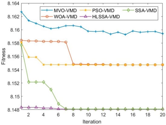
Figure 15. The iterative optimization process of the five algorithms.

Table 7. The optimization results obtained with the five algorithms.

Methods	Fitness	[K, α]
MVO-VMD	8.15943	[6, 1033]
PSO-VMD	8.15474	[6, 1097]
WOA-VMD	8.15474	[6, 1097]
SSA-VMD	8.14811	[6, 1236]
HLSSA-VMD	8.14811	[6, 1236]

From Table 7, it is evident that both the SSA and HLSSA demonstrated superior performance in terms of convergence accuracy. However, as shown in Figure 15, the HLSSA outperformed the SSA regarding initialization and convergence speed. This indicates that the proposed improvement to the SSA is effective, and the HLSSA demonstrates higher-quality initialization, faster convergence speed, and superior convergence accuracy.

The second set of simulated signals consisted of three signals with different frequencies that were superimposed at different time intervals. To simulate real-world signals more accurately, Gaussian white noise was added to the signal s. The construction process of signal s is as follows:

$$\begin{array}{l}{s}_1=1.5\sin (100\pi t)\\ s_2=2\sin (300\pi t)\\ s_3=\sin (500\pi t)\\ s_4=2.5\sin (700\pi t)\\ s=s_1+s_2+s_3+s_4+s_5\end{array}$$

(13)

where $s_5$ is a Gaussian white noise signal with a mean of 0 and a standard deviation of 1.

Figure 16a is a visual representation of each simulated signal. Signal $s_1$ had an amplitude of 1.5, a frequency of 50 Hz, and a duration of 0–1 s; signal $s_2$ had an amplitude of 2, a frequency of 150 Hz, and a duration of 0.35–0.65 s; signal $s_3$ had an amplitude of 1.5, a frequency of 250 Hz, and a duration of 0.15–0.5 s; and signal $s_4$ had an amplitude of 2.5, a frequency of 350 Hz, and a duration of 0.4–0.8 s. Figure 16b shows the amplitude–frequency plot obtained by performing a Fourier transform on the synthesized signal s. Figure 16b demonstrates that the synthesized signal s contained the frequencies corresponding to the simulated signals $s_1-s_4$.

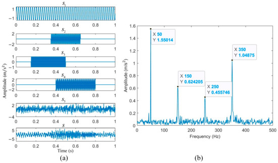
Figure 16. (a) Simulated signal; (b) amplitude–frequency plot of the synthesized signal s.

The optimal parameters K and α for the VMD algorithm in decomposing signal s were obtained using the HLSSA. The search ranges for K and α were set to [100, 6000] and [1, 10], respectively. Figure 17 illustrates the iterative optimization process for the five algorithms, and Table 8 presents the optimal solutions obtained with each algorithm.

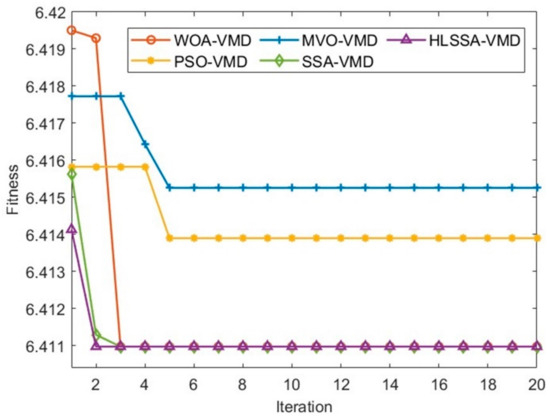
Figure 17. The iterative optimization process of the five algorithms.

Table 8. The optimization results obtained with the five algorithms.

Methods	Fitness	[K, α]
MVO-VMD	6.4152	[3, 5803]
PSO-VMD	6.4139	[4, 3361]
WOA-VMD	6.410	[4, 6000]
SSA-VMD	6.410	[4, 6000]
HLSSA-VMD	6.410	[4, 6000]

As shown in Figure 17 and Table 8, the MVO and PSO exhibited relatively poorer convergence accuracy, while the WOA, SSA, and HLSSA yielded the same optimization results. However, the HLSSA demonstrated a faster convergence speed, and it had the lowest initial fitness value, indicating that the HLSSA provides a higher quality initial solution.

In Figure 18a, the decomposition results of MVO-VMD are displayed, revealing that the algorithm only decomposed three signals of different frequencies, while the 250 Hz signal was absent. Figure 18b shows the decomposition results of PSO-VMD, and although it successfully decomposed the signals of four different frequencies, each frequency component exhibited significant jitter, resulting in less smooth decomposition. Figure 18c–e demonstrate the decomposition results of WOA-VMD, SSA-VMD, and HLSSA-VMD, respectively. In contrast to PSO-VMD, these three algorithms not only successfully decomposed all frequencies but also provided smoother decomposition results, indicating superior performance.

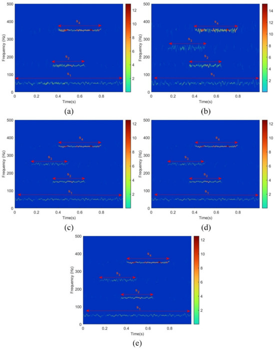
Figure 18. Hilbert spectra corresponding to different algorithms: (a) MVO-VMD; (b) PSO-VMD; (c) WOA-VMD; (d) SSA-VMD; (e) HLSSA-VMD.

This comparative analysis further validates the outstanding performance of the HLSSA in optimizing VMD parameters, showcasing its faster convergence speed and higher-quality decomposition results.

5. Conclusions

In this study, we proposed the HLSSA-VMD algorithm for optimizing VMD parameters. Firstly, we validated the performance of the HLSSA across 17 benchmark functions, demonstrating its superiority in convergence accuracy, convergence speed, and robustness compared to the PSO, WOA, MVO, and SSA. Secondly, we evaluated the performance of the HLSSA-VMD algorithm on two simulated signals, revealing that, in comparison with other algorithms, HLSSA-VMD effectively enhances VMD’s parameter optimization capabilities and improves signal decomposition quality.

References

- Deng, L.; Liu, S. A Novel Hybrid Grasshopper Optimization Algorithm for Numerical and Engineering Optimization Problems. Neural Process. Lett. 2023, 55, 9851–9905. [Google Scholar] [CrossRef]
- Wang, X.; Zhou, F.; He, Y.; Wu, Y. Weak Fault Diagnosis of Rolling Bearing under Variable Speed Condition Using IEWT-Based Enhanced Envelope Order Spectrum. Meas. Sci. Technol. 2019, 30, 035003. [Google Scholar] [CrossRef]
- Xu, Y.; Cai, Z.; Ding, K. An Enhanced Bearing Fault Diagnosis Method Based on TVF-EMD and a High-Order Energy Operator. Meas. Sci. Technol. 2018, 29, 095108. [Google Scholar] [CrossRef]
- Chegini, S.N.; Bagheri, A.; Najafi, F. Application of a New EWT-Based Denoising Technique in Bearing Fault Diagnosis. Measurement 2019, 144, 275–297. [Google Scholar] [CrossRef]
- Keyhani, A.; Mohammadi, S. Structural Modal Parameter Identification Using Local Mean Decomposition. Meas. Sci. Technol. 2018, 29, 025003. [Google Scholar] [CrossRef]
- Dragomiretskiy, K.; Zosso, D. Variational Mode Decomposition. IEEE Trans. Signal Process. 2014, 62, 531–544. [Google Scholar] [CrossRef]
- Wang, W.; Guo, S.; Zhao, S.; Lu, Z.; Xing, Z.; Jing, Z.; Wei, Z.; Wang, Y. Intelligent Fault Diagnosis Method Based on VMD-Hilbert Spectrum and ShuffleNet-V2: Application to the Gears in a Mine Scraper Conveyor Gearbox. Sensors 2023, 23, 4951. [Google Scholar] [CrossRef]
- Luo, J.; Wen, G.; Lei, Z.; Su, Y.; Chen, X. Weak Signal Enhancement for Rolling Bearing Fault Diagnosis Based on Adaptive Optimized VMD and SR under Strong Noise Background. Meas. Sci. Technol. 2023, 34, 064001. [Google Scholar] [CrossRef]
- Zhang, M.; Cao, Y.; Sun, Y.; Su, S. Vibration Signal-Based Defect Detection Method for Railway Signal Relay Using Parameter-Optimized VMD and Ensemble Feature Selection. Control Eng. Pract. 2023, 139, 105630. [Google Scholar] [CrossRef]
- Li, T.; Zhang, F.; Lin, J.; Bai, X.; Liu, H. Fading Noise Suppression Method of Φ-OTDR System Based on Non-Local Means Filtering. Opt. Fiber Technol. 2023, 81, 103572. [Google Scholar] [CrossRef]
- Liu, B.; Liu, C.; Zhou, Y.; Wang, D. A Chatter Detection Method in Milling Based on Gray Wolf Optimization VMD and Multi-Entropy Features. Int. J. Adv. Manuf. Technol. 2023, 125, 831–854. [Google Scholar] [CrossRef]
- Mao, M.; Chang, J.; Sun, J.; Lin, S.; Wang, Z. Research on VMD-Based Adaptive TDLAS Signal Denoising Method. Photonics 2023, 10, 674. [Google Scholar] [CrossRef]
- Lu, D.; Shen, S.; Li, Y.; Zhao, B.; Liu, X.; Fang, G. An Ice-Penetrating Signal Denoising Method Based on WOA-VMD-BD. Electronics 2023, 12, 1658. [Google Scholar] [CrossRef]
- Jin, Z.; He, D.; Ma, R.; Zou, X.; Chen, Y.; Shan, S. Fault Diagnosis of Train Rotating Parts Based on Multi-Objective VMD Optimization and Ensemble Learning. Digit. Signal Process. 2022, 121, 103312. [Google Scholar] [CrossRef]
- Jing, L.; Bian, J.; He, X.; Liu, Y. Study on the Optimization of the Classification Method of Rolling Bearing Fault Type and Damage Degree Based on SFO–VMD. Meas. Sci. Technol. 2023, 34, 125047. [Google Scholar] [CrossRef]
- Wang, J.; Zhan, C.; Li, S.; Zhao, Q.; Liu, J.; Xie, Z. Adaptive Variational Mode Decomposition Based on Archimedes Optimization Algorithm and Its Application to Bearing Fault Diagnosis. Measurement 2022, 191, 110798. [Google Scholar] [CrossRef]
- Xue, J.; Shen, B. A Novel Swarm Intelligence Optimization Approach: Sparrow Search Algorithm. Syst. Sci. Control Eng. 2020, 8, 22–34. [Google Scholar] [CrossRef]
- Gao, B.; Shen, W.; Guan, H.; Zheng, L.; Zhang, W. Research on Multistrategy Improved Evolutionary Sparrow Search Algorithm and Its Application. IEEE Access 2022, 10, 62520–62534. [Google Scholar] [CrossRef]
- Geng, J.; Sun, X.; Wang, H.; Bu, X.; Liu, D.; Li, F.; Zhao, Z. A Modified Adaptive Sparrow Search Algorithm Based on Chaotic Reverse Learning and Spiral Search for Global Optimization. Neural Comput. Applic. 2023, 35, 24603–24620. [Google Scholar] [CrossRef]
- Du, Y.; Yuan, H.; Jia, K.; Li, F. Research on Threshold Segmentation Method of Two-Dimensional Otsu Image Based on Improved Sparrow Search Algorithm. IEEE Access 2023, 11, 70459–70469. [Google Scholar] [CrossRef]
- Xiong, Q.; Zhang, X.; He, S.; Shen, J. A Fractional-Order Chaotic Sparrow Search Algorithm for Enhancement of Long Distance Iris Image. Mathematics 2021, 9, 2790. [Google Scholar] [CrossRef]
- Sun, H.; Wang, J.; Chen, C.; Li, Z.; Li, J. ISSA-ELM: A Network Security Situation Prediction Model. Electronics 2022, 12, 25. [Google Scholar] [CrossRef]
- Han, M.; Zhong, J.; Sang, P.; Liao, H.; Tan, A. A Combined Model Incorporating Improved SSA and LSTM Algorithms for Short-Term Load Forecasting. Electronics 2022, 11, 1835. [Google Scholar] [CrossRef]
- Jianhua, L.; Zhiheng, W. A Hybrid Sparrow Search Algorithm Based on Constructing Similarity. IEEE Access 2021, 9, 117581–117595. [Google Scholar] [CrossRef]
- Hanh, N.T.; Binh, H.T.T.; Hoai, N.X.; Palaniswami, M.S. An Efficient Genetic Algorithm for Maximizing Area Coverage in Wireless Sensor Networks. Inf. Sci. 2019, 488, 58–75. [Google Scholar] [CrossRef]
- Ul Haq, E.; Ahmad, I.; Almanjahie, I.M. A Novel Parent Centric Crossover with the Log-Logistic Probabilistic Approach Using Multimodal Test Problems for Real-Coded Genetic Algorithms. Math. Probl. Eng. 2020, 2020, 1–17. [Google Scholar] [CrossRef]
- Deep, K.; Thakur, M. A New Crossover Operator for Real Coded Genetic Algorithms. Appl. Math. Comput. 2007, 188, 895–911. [Google Scholar] [CrossRef]
- Thakur, M.; Meghwani, S.S.; Jalota, H. A Modified Real Coded Genetic Algorithm for Constrained Optimization. Appl. Math. Comput. 2014, 235, 292–317. [Google Scholar] [CrossRef]
- Emami, M.; Mozaffari, A.; Azad, N.L.; Rezaie, B. An Empirical Investigation into the Effects of Chaos on Different Types of Evolutionary Crossover Operators for Efficient Global Search in Complicated Landscapes. Int. J. Comput. Math. 2016, 93, 3–26. [Google Scholar] [CrossRef]
- Halton, J.H. Algorithm 247: Radical-Inverse Quasi-Random Point Sequence. Commun. ACM 1964, 7, 701–702. [Google Scholar] [CrossRef]
- Halton, J.H. On the Efficiency of Certain Quasi-Random Sequences of Points in Evaluating Multi-Dimensional Integrals. Numer. Math. 1960, 2, 84–90. [Google Scholar] [CrossRef]
- Kocis, L.; Whiten, W.J. Computational Investigations of Low-Discrepancy Sequences. ACM Trans. Math. Softw. 1997, 23, 266–294. [Google Scholar] [CrossRef]
- Tian, S.; Zhen, D.; Liang, X.; Feng, G.; Cui, L.; Gu, F. Early Fault Feature Extraction for Rolling Bearings Using Adaptive Variational Mode Decomposition with Noise Suppression and Fast Spectral Correlation. Meas. Sci. Technol. 2023, 34, 065112. [Google Scholar] [CrossRef]
Disclaimer/Publisher’s Note: The statements, opinions and data contained in all publications are solely those of the individual author(s) and contributor(s) and not of MDPI and/or the editor(s). MDPI and/or the editor(s) disclaim responsibility for any injury to people or property resulting from any ideas, methods, instructions or products referred to in the content. |
© 2024 by the authors. Licensee MDPI, Basel, Switzerland. This article is an open access article distributed under the terms and conditions of the Creative Commons Attribution (CC BY) license (https://creativecommons.org/licenses/by/4.0/).