The Numerical Analysis of Textile Reinforced Concrete Shells: Basic Principles

Abstract

In the case of solid slabs made from reinforced concrete that are usually subjected to bending, large areas of the structure are stressed well below their load-bearing capacity or remain stress-free. Contrary to this are shell structures, which can bridge large spans with little material if designed well. To improve the efficiency of ceiling slabs, we want to utilize the shell load-bearing behaviour on a smaller scale by dissolving the solid interior accordingly. In order to be able to study a wide range of such constructions virtually, a parametric multi-objective simulation environment is to be developed in an ongoing research project, the basic analysis approaches of which are presented in this paper. In addition to the basic workflow and the programs used, the material models for TRC material compared and their calibration are described on the basis of tests on textile reinforced concrete (TRC) samples. Various material models were implemented within the commercially available software RFEM (Version 5.19). Laboratory tests on two different geometry solutions of TRC structures served to verify the models. The structures were selected in a way that differentiates between the bending and membrane actions to indicate the application fields for various approaches in the numerical modelling of TRC structures.

1. Introduction

Ceiling slabs made from reinforced concrete usually have a constant, solid cross-section. Under pure bending stress, which is the usual case, many sections of the structure are loaded well below their load-bearing capacity or remain free of stress. Overall, the material utilization is not efficient, and there is a large self-weight. This is fundamentally contrary to the modern necessity to use resources of all kinds as efficiently as possible.

Various methods are known to increase the efficiency of concrete components subjected to bending. These methods are often based on the principle ‘form follows force’ or the intelligent combination of materials with different densities and mechanical properties. Examples are outlined in Refs. [1,2,3] (adaptation of the outer geometry of a component), [4,5] (sandwich-like layering of different concretes), and [6,7,8] (inner hollow spaces, generated by hollow bodies, or grading for weight minimization).

In the project C01 of the CRC/Transregio 280 “Design Strategies for Material-Minimized Carbon-Reinforced Concrete Structures—Principles of a New Approach to Construction” [9,10], a new approach is being explored. We intend to use the outstanding load-bearing behaviour of shell constructions on a smaller scale using textile reinforced concrete (TRC). If the shell shape is adjusted so that the resultant of the decisive continuously acting loads remains in the core cross-section, normal forces predominate. The material is utilized homogeneously (a membrane stress condition). The three-dimensional shape provides stability. This project aims to exploit this load-bearing principle of shells at the component level. The idea is to dissolve the usually solid interior of, e.g., a plate subject to bending into load-bearing shell structures [11]. Thus, the material is used more efficiently, and weight is saved at the same time, without any loss in load-bearing capacity. This paper discusses the basic principles that form the analysis routines to aim reaching this goal.

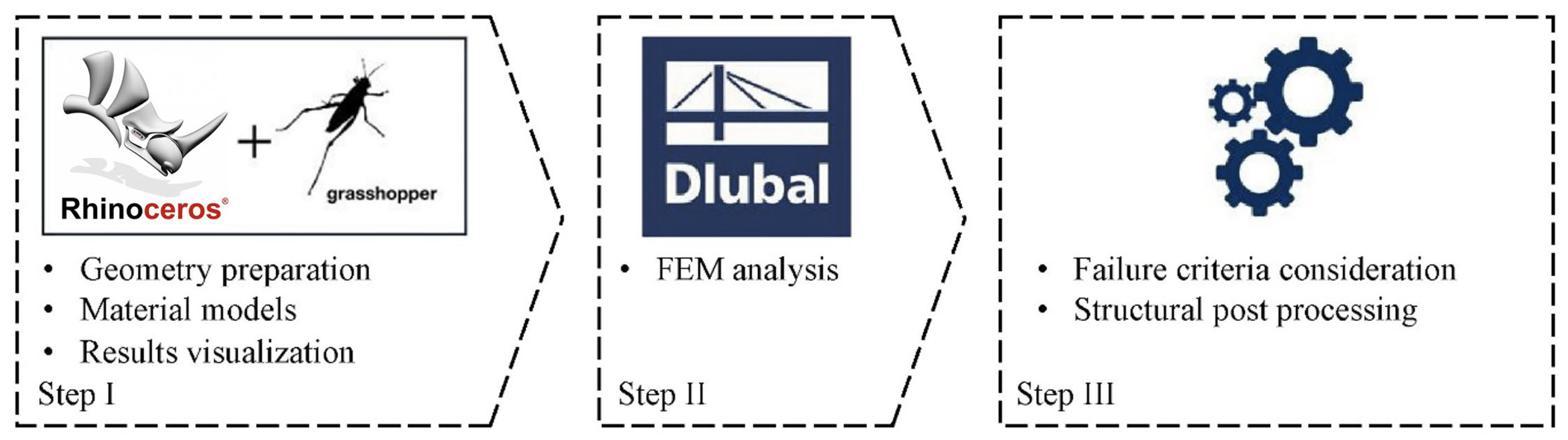
2. Workflow Overview

One of the most important aspects of the development of a method to deal with curved filigree TRC structures within the scope of the project is the computational workflow that determines how to calculate such structures. The process was developed in the form of three steps. Figure 1 gives a general overview of the steps and their constituent subroutines.

In the first step, the basic geometrical principles of the TRC shell structure are described using the parametric environments of Rhino 3D (Ver. 7.0) [12] and Grasshopper 3D (Ver. 7.0) [13] (Rh + GH) software packages. Furthermore, Rh + GH processes the other model metadata such as material properties, load cases, boundary conditions, etc. The second step starts when all the required information about the structural model is transferred to the FEM software via the COM interface [14]. Considering two recently successfully finished projects [15,16], the software RFEM (Ver.5.19) [17] from Dlubal Software, Inc. (Tiefenbach, Germany). was selected for the current research project. The usage of RFEM as a main FEM solver provides competitively fast processing and stability. The raw data processing from the FEM calculator occurs in Step III. The standalone programs analyse the failure criterion and the utilization ratio and prepare a visualization of the FEM results as well as required statistics. If the failure load is not reached, the process may be performed iteratively between Step II and Step III until the failure of the structure is recognized by the failure criteria programmed modules.

It is important to specify that one part of the components of the calculation routines were directly developed within the Rh + GH environment and another part was implemented in the form of external solutions based on Python or C# programming languages. Such an approach helps to improve the processing speed of the components and make them more independent from each other, which, in turn, adds modularity features to the whole system. The modularity of the workflow supports the integration of more sophisticated analysis methods and failure criteria for TRC structures such as those described in ref. [18].

3. Materials Models

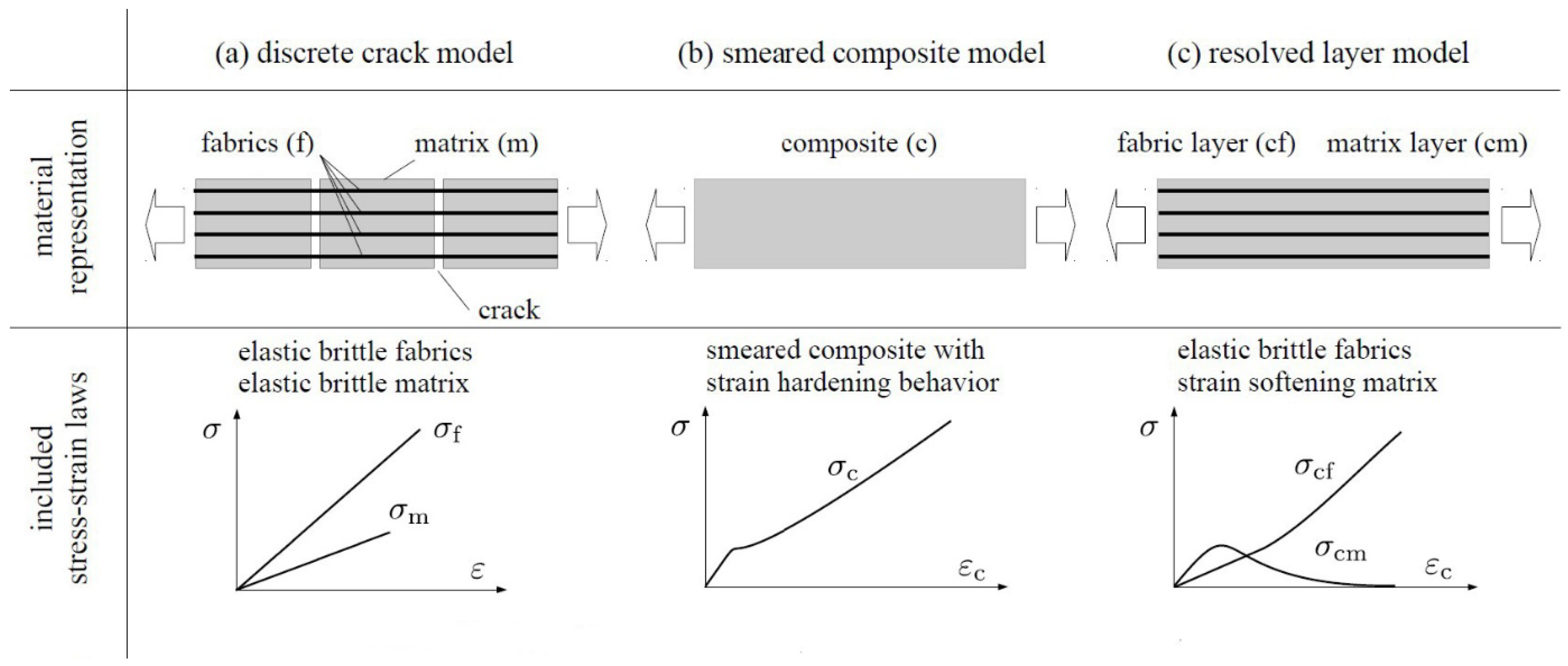
3.1. Short Overview of Material Models for TRC

One of the most important points is the way the calculation routines integrate the theoretical background of the TRC structures. In the present state of the art in the field of the analysis of TRC structures, three categories of numerical approaches can be summarized [19] which are given in Figure 2 as a schematic overview. The first column (a) shows parameters of the discrete crack model description. Here, the damage to the concrete is considered via the evolution of discrete cracks in the matrix and a nonlinear bond stress–slip relation between concrete and continuous fibre-based reinforcement [19]. The model gives a valuable representation of the composite behaviour but with a considerable level of complexity in the description of the governing mechanisms as well as computational efforts. For the planned iterative workflow, a high numerical complexity implies a disproportionate numerical effort, which is why this approach was not pursued further for the project. In the smeared model (b), TRC is represented as a composite with uniform behaviour over the cross-section. The model’s parameters are determined via the rule of mixtures that demands the correct estimation of the volume fractions of the constituents. With that, the material model has to be calculated for each cross-sectional configuration [19]. It should be noted here that the smeared model was the most convenient one within the selected software packages to account for the damage effects in the TRC. A more detailed description of the model used in RFEM is given later. The third model (c) contains a resolved realization of the matrix and textile layers. This behaviour is similar to the discrete model with the difference that the cracks in the matrix are smeared along the specimen. This makes the model less demanding for the numerous calibration procedures and gives the opportunity to consider the exact position of the reinforcement layers within the cross-section [19].

For the calculation in RFEM, a material description for the composite textile reinforced concrete under compressive and tensile stress is required which can be represented by the smeared approach. The stress–strain behaviour of TRC under tension is very similar to that of steel-reinforced concrete, see, e.g., refs. [20,21]. In State I, the concrete is non-cracked, and the specimen’s stiffness is high. The composite’s strain ${\epsilon }_c$ is equal to the strains in matrix ${\epsilon }_m$ and the fibre reinforcement ${\epsilon }_f$. When the concrete’s tensile strength is reached, cracks begin to form successively (State IIa). If the tensile force is increased further beyond the point of completed cracking, the number of cracks no longer changes. Only the crack widths increase (State IIb) until the textile tears. Since, in this state, only textile reinforcement bears the total tensile load, the composite section possesses the stiffness of the reinforcement. As part of the described workflow (Figure 1), a special script was developed within the scope of the Rh + GH environment, with which multiple experimental results of a test series were converted into a single average curve of the stress–strain relation. Afterwards, the script converts this average data curve into three states, I to IIb, to be able to map the curve analytically for further processing.

The analytical description should reflect the material behaviour of TRC as accurately as possible. This is important for the further optimization and analysis of the textile reinforced concrete shell structures in the context of a theoretical parametrical study, as only singular structures can be tested in the experiment. However, we would like to be able to make a statement about the behaviour of structures with different geometries, material combinations and loading scenarios. There are several analytical models appropriate for TRC, each with specific advantages and disadvantages. The following two were shortlisted:

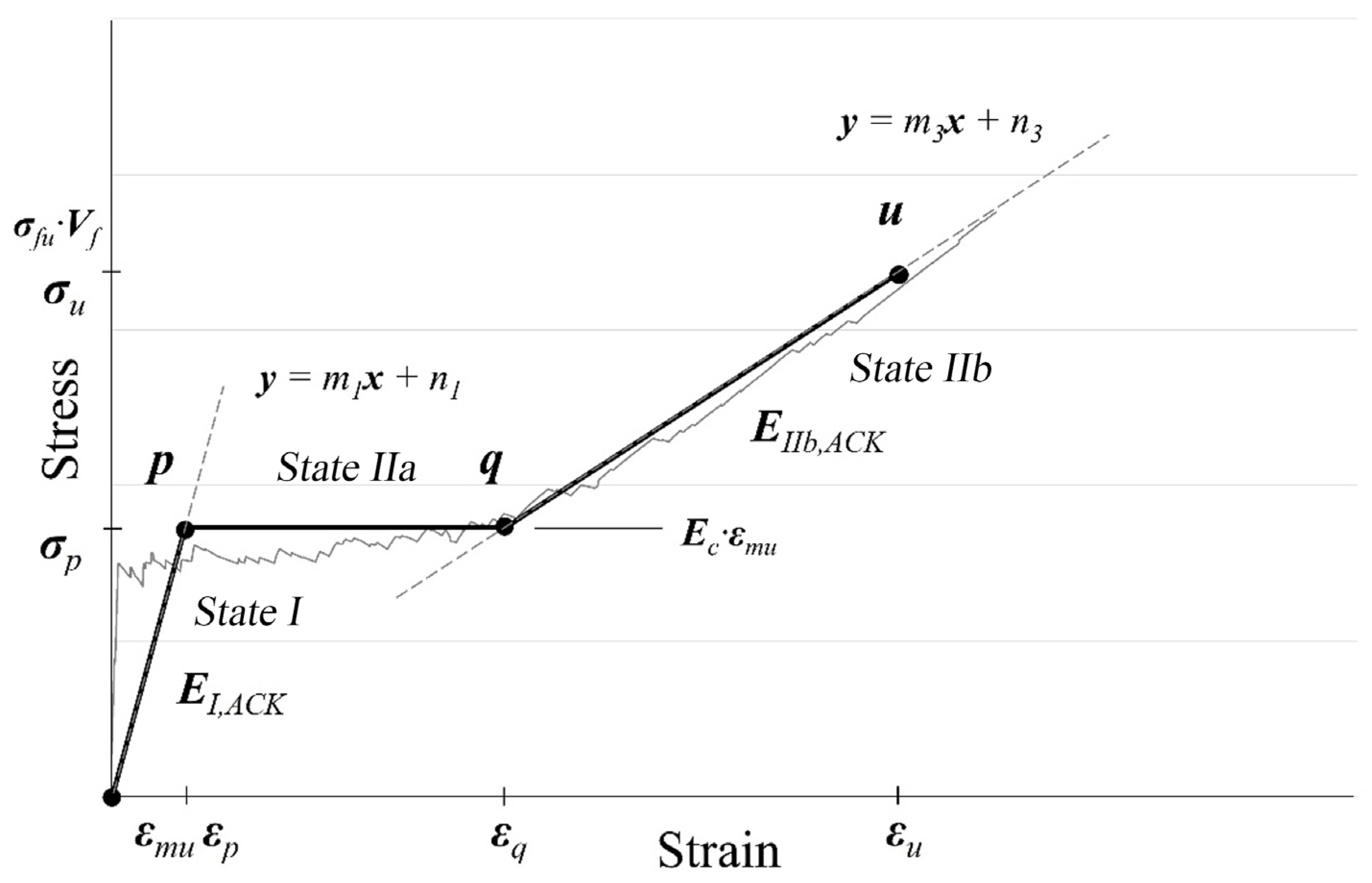
• The ACK model is named after its creators, Aveston, Cooper, and Kelly, and was published in 1971. The key aspect of the model is that it is one of the most numerically simple and is based on simplified assumptions describing the processes that occur inside the TRC sample under the tensile action [20].
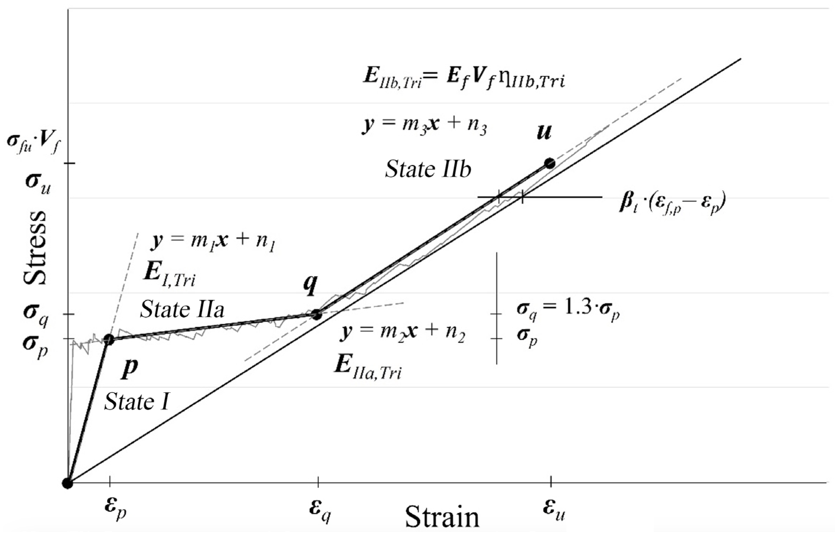
• The trilinear model is based on the approach of three linear, continuously ascending ranges which are adapted from the real stress–strain line of TRC. The slope and other parameters can be determined according to the rule of mixtures, appropriate efficiency factors, and recommendations from Model Code 90 [22,23,24].

The common approach, valid for each of the material models, is that the experimental data can be approximated by idealized first-order polynomials, e.g., see ref. [20]:

$${\mathit{y}}_{\mathit{i}}=m·{\mathit{x}}_{\mathit{i}}+n$$

(1)

where the coefficients $m$ and $n$ determine the slope and the intercept of the polynomial, respectively, and ${\mathit{y}}_{\mathit{i}}$ and ${\mathit{x}}_{\mathit{i}}$ are experimental data points.

3.2. ACK Material Model

The ACK model possesses one key feature: a simple analytical assembly. The simplicity is governed by accepted assumptions such as the perfect bond between the matrix and fibres, behaviour according to the theory of elasticity, the law of mixtures, and the assumption of essentially constant stress level in the crack formation phase (State IIa) [20]. Figure 3 shows the principal behaviour with all the respective components.

Based on experimental data, the coefficients of the first-order polynomial equations can be calculated in general form using linear regression principles with the least squares method. The experimental data and least squares method give $E$ modulus values for the TRC material only for State I and State IIb according to the assumptions made previously. The respective values can be expressed as follows:

$$E_{I,ACK}=E_f·V_f+E_m·\left(1-V_f\right)$$

(2)

$$E_{IIb,ACK}=E_f·V_f·{\eta }_{IIb,ACK}$$

(3)

where $E_{I,ACK} \left(\mathrm{M}\mathrm{P}\mathrm{a}\right)$ and $E_{IIb,ACK} \left(\mathrm{M}\mathrm{P}\mathrm{a}\right)$ are the composite’s stiffnesses of a TRC sample in State I and State IIb respectively; $V_f$ symbolizes the fibre volume fraction calculated as $V_f=A_{tex}/A_c$, with $A_{tex}$ being the cumulative area of the textile reinforcement and $A_c$ being the total sample cross-section in (mm²); ${\eta }_{IIb,ACK}$ is an efficiency factor of the textile reinforcement. The expressions given in Equations (2)–(3) are derived based on the common principles of ACK model construction, as described in refs. [22,25,26]. The recent research in the field of TRC [20] proposes the modification of the ACK model with an efficiency factor that can be explained with the influence of the failure of sleeve fibres and the bundle effect [27]. For a proper determination of the multi-linear law, the transition points have to be located as follows:

$${\epsilon }_p=\frac{{\sigma }_{mu}}{E_m}$$

(4)

$${\epsilon }_q=\frac{{\sigma }_{mu}}{E_f·V_f·{\eta }_{IIb,ACK}}-{C·\alpha }_e·{\sigma }_{mu}$$

(5)

where ${\sigma }_{mu} \left(\mathrm{M}\mathrm{P}\mathrm{a}\right)$ is the matrix tensile strength at failure (first crack) and ${\epsilon }_p$ and ${\epsilon }_q$ are strain levels for points p and q, according to Figure 3. The numerical constant C depends on the crack spacing and has to be calibrated. The given calculation concept can be used to derive the stress–strain relation of composites with various fibre types [22]. The homogenization coefficient ${\alpha }_e$ can be calculated via Equation (6):

$${\alpha }_e=\frac{E_m·\left(1-V_f\right)}{E_f·V_f·{\eta }_{IIb,ACK}}$$

(6)

The ultimate point u defines the tensile limit of the composite material. The associated material values are as follows:

$${\sigma }_u={\sigma }_{u,tex}·V_f·{\eta }_{IIb,ACK}$$

(7)

$${\epsilon }_u={\epsilon }_q+\frac{{\sigma }_u-{\sigma }_q}{E_f·{\eta }_{IIb,ACK}}$$

(8)

where ${\sigma }_{u,tex}$ is the tensile limit of the textile reinforcement in MPa.

3.3. Trilinear Material Model

An alternative concept for modelling the tensile behaviour of TRC composites is a solution introduced by Nathan et al. [23] in 1977 using a trilinear stress–strain curve characterized by three linear ranges similar to that of the ACK model [22]. However, the line in the second area is not horizontal but slightly ascending (Figure 4). The slope of the line in each range is calculated in a similar way using a rule of mixtures, combined with the appropriate efficiency factors. The determination of the factors is the objective for further material model calibration.

The trilinear material model gives a similar representation for the uncracked zone to the ACK model. The reason for that similarity lies in the basic principles that describe the material according to the rule of mixtures and the joint assumption that until the initiation of a first crack in the composite, the compatibility of strain between the fibre and the matrix is satisfied [23]. Thus, the strain level ${\epsilon }_p$ for point p can be similarly calculated via Equation (10) with the respective levels of the matrix tensile strength ${\sigma }_{mu}$ and elastic modulus $E_{I,Tri} \left(\mathrm{M}\mathrm{P}\mathrm{a}\right)$ for the uncracked range in State I. In the further description, the rules are based on Model Code 90 guidelines for tension-stiffening effects according to refs. [5,24]. The next point q with ${\sigma }_q$ and ${\epsilon }_q$ can be calculated using Equations (9) and (10) [28]:

$${\sigma }_q=1.3·{\sigma }_p$$

(9)

$${\epsilon }_q={\epsilon }_{f,q}-∆\epsilon$$

(10)

where ${\epsilon }_{f,q}$ is the strain of the reinforcement in a crack. For the calculation of the composite’s strain in point q, at first, the strain of the pure reinforcement is calculated for the loading at this load level ${\sigma }_q$. The associated strains differ between embedded reinforcement and pure respective unembedded grid. The difference $∆\epsilon$ reflects the influence of the tension stiffening effect and may be considered via the following:

$$∆\epsilon ={\beta }_t·\left({\epsilon }_{f,p}-{\epsilon }_p\right)$$

(11)

where ${\beta }_t$ is the integration factor for the reinforcement strain along the transmission length; ${\epsilon }_{f,p}$ is the fibre strain at the point of zero slip under first crack forces reaching ${\sigma }_{mu}$; and ${\epsilon }_p$ is the fibre strain in the crack under cracking stress reaching $f_{\mathrm{c}\mathrm{t}\mathrm{m}}\left(t\right)$ [24]. A factor of 1.3 is recommended as the difference between ${\sigma }_p$ and ${\sigma }_q$ for TRC samples according to [20]. In addition, the composite’s stiffness $E_{IIa}$ in the area of successive crack formation after the first crack can be described using the principle of first-order polynomial approximation as follows:

$$E_{IIa,Tri}={k·E}_m·V_m+E_f·V_f$$

(12)

where $k<1$ is an empirical parameter accounting for the reduction in the effectiveness of the concrete matrix [29]. The value of $k$ is dependent on the volume fraction of fibres $V_f$ and can be determined, e.g., experimentally. Thus, the value ${\sigma }_p$ may be alternatively determined via the intersection of the two first-order polynomial functions that describe State IIa with a slope of $E_{IIa,Tri}$ and State IIb with a slope of $E_{IIb,Tri}$. There are two close approaches: one based on Model Code 90, Equation (9), and the other based on the geometrical interpretation of Equation (12). Furthermore, the strain in the State IIa range can be estimated in practical way with Equation (13):

$$\epsilon ={\epsilon }_{f,p}-\frac{{\beta }_t·\left(\sigma -{\sigma }_p\right)+\left({\sigma }_q-\sigma \right)}{{\sigma }_q-{\sigma }_p}·\left({\epsilon }_{f,p}-{\epsilon }_p\right)$$

(13)

with ${\sigma }_p<\sigma \le {\sigma }_q$ and ${\epsilon }_p<\epsilon \le {\epsilon }_q$. Hence, the slope of the polynomial of the composite $E_{IIb,Tri}$ corresponds to a parallel shift in the polynomial of the unembedded reinforcement that is described according to the rule of mixtures similarly to the ACK model as follows:

$$E_{IIb,Tri}=E_f·V_f·{\eta }_{IIb,Tri}$$

(14)

where the experimental factor ${\eta }_{III,Tri}$ considers the reduction in the stiffness similarly due to the textile reinforcement bundle effect [27]. The ultimate tensile point u and the respective values of the ultimate stress ${\sigma }_u$ and strain ${\epsilon }_u$ should be determined similarly according to the Equations (7) and (8), respectively.

3.4. Calibrating the Selected Material Models

To calibrate the material models and respective parameters, it was necessary to perform uniaxial tensile tests on composite samples. The concrete mixture C3-B2-HF-2-190-2 [30], optimized for fibre reinforcement, was used. With a maximum grain size of 2 mm, it is also suitable for the production of very intricate concrete components.

Table 1. Mixture composition of concrete C3-B2-HF-2-190-2 [30].

Raw Materials	Quantity (kg/m³)
Binder compound BMK-DS-1 (Dyckerhoff, Germany)	815
Quartz sand 0.06/0.2	340
Sand 0/2	965
Superplasticizer (e.g., MC-VP-16-0205-02 from MC-Bauchemie, Germany)	17
Water	190

provides the mixture composition [30]. The binder BMK-D5-1 is outside the current cement standard due to the addition of an inert filler and was developed in a partnership between the Institute for Building Materials of TU Dresden and the Deuna cement plant (Dyckerhoff^® company, Wiesbaden, Germany) in the project C3-B2 as part of the C³—Carbon Concrete Composite project [31].

The compressive and bending tensile strengths of the hardened concrete from

Table 2. Properties of hardened concrete (mean values).

Property	Value	Unit
Compressive strength fcm	114.8	MPa
Bending tensile strength fctm, fl	8.8	MPa

were determined on three prisms with dimensions of 40 × 40 × 160 mm according to DIN EN 196-1 [32].

As a carbon fibre textile reinforcement, the solidian GRID Q85-CCE-21-E5 [33] was selected. The factory-guaranteed properties are provided in

Table 3. Properties of textile reinforcement solidian GRID Q85-CCE-21 [33].

Property	Longitudinal	Transversal
Roving axis distance etex (mm)	21	21
Cross-section of a roving Af (mm2)	1.81	1.81
Cross-section of the reinforcement grid Atex (mm2/m)	85.4	85.6
Tensile strength of the roving σu,f (MPa)	≥3950	≥4250
Tensile strength of the grid σu,tex (MPa)	≥3950 (avg.)|≥3050 (char.)	≥4250 (avg.)|≥3250 (char.)
Resisting force Ftex (kN/m)	≥260.5	≥275.0
Modulus of elasticity Etex (MPa)	≥251,500	≥254,000

[33].

For tensile tests on TRC, a 1220 × 540 × 40 mm slab was concreted and stored for the first few days under wet cloths and afterwards at 20 °C in a climate chamber with 65% relative humidity. The plate thickness and the two-layer carbon reinforcement were selected according to shell elements planned for subsequent steps. The reinforcement was located centrally with a gap of 10 mm, and the concrete covers were equal to 15 mm on both sides of the test samples. Before testing at an age of 28 days, in total, six tensile test samples with dimensions of 800 × 62 × 40 mm were cut off from the slab. The samples were displacement-controlled loaded with a loading speed of 0.03 mm/min until failure. In addition to the force, the deformation was recorded using two LVDTs in the measuring range. The test setup is presented in Figure 5.

The average stress–strain curve from the six individual tests is compared with the material models in the following, and the detailed results are published in [34]. Based on the material properties presented, the material models described above were calibrated. Figure 6 shows the results for the ACK material model (M1). Similarly, Figure 7 displays simulated results for the trilinear model (M2). For the comparison with the experiments, both models were calibrated with $V_f=0.40\%$.

The key characteristic values of the calibrated material models are compiled in

Table 4. Calibrated parameters of the material models.

Properties	ACK	Trilinear
$E_I$ (MPa)	42,100.0	42,100.0
$E_{IIa}$ (MPa)	0.0	201.14
$E_{IIb}$ (MPa)	846.9	843.28
${\eta }_{IIb}$	0.91	0.91
C	−0.02	–
${\beta }_t$	–	−0.04
k	–	0.0025

. As expected, the most significant difference between the two models can be seen in State IIa. The M2 model can clearly represent the real material behaviour in this area better than the M1 model. To observe the key role the model plays within the scope of numerical analysis, see Section 6.

Though the analytical material models significantly simplify the calculation routine, in some features, they show some differences to the experimental results. Thus, for instance, for the point p that depicts the transition from State I to State IIa, the stress level ${\sigma }_{mu}$ is equal to the tensile strength of the concrete matrix $f_{ctm}$. It can be calculated using results derived for the prism tests given in Table 2 according to Equation (15) [24,28]:

$$f_{ctm,prism}=f_{ctm,fl}·\frac{1.5·{\left(\frac{h_b}{h_0}\right)}^{0.7}}{1+1.5·{\left(\frac{h_b}{h_0}\right)}^{0.7}}$$

(15)

where the height of the prism $h_b$ = 40 mm and the standard coefficient $h_0$ = 100 mm according to [24]. Thus, $f_{ctm,prism}$ = 3.88 MPa, which does not match with the first crack tensile stress obtained in the series of the uniaxial experiments equal to $f_{ctm,exp}$ = 5.64 MPa. To overcome the presented weak aspect of the material models, it is recommended to use the experimental first crack stress for the material model assembly given by ${\sigma }_{mu}=f_{ctm,exp}$ [20,35].

The selected textile reinforcement behaviour is assumed to be linear [36] for the provided calculations with an elastic modulus $E$ of 251.5 GPa, according to Table 3. To simplify, the concrete behaviour under pressure is modelled using a bilinear approach, considering a mean compression strength value of $f_{\mathrm{c}\mathrm{m}}=$ 114.8 MPa. Furthermore, the material density ${\rho }_c$ of the concrete taken from the standard prisms with 2340 kg/m³ was included in the FEM model.

4. FEM Model Formulation

As mentioned previously, the commercial software RFEM (Ver. 5.19) [17] was selected for the FE calculations. The software package possesses a set of materials models with different drawbacks and benefits. The TRC material behaviour can be used as an input. In the following, we provide an overview of the three most feasible material models available in the user interface of RFEM which were verified to be used for the simulation of TRC structures via the smeared approach.

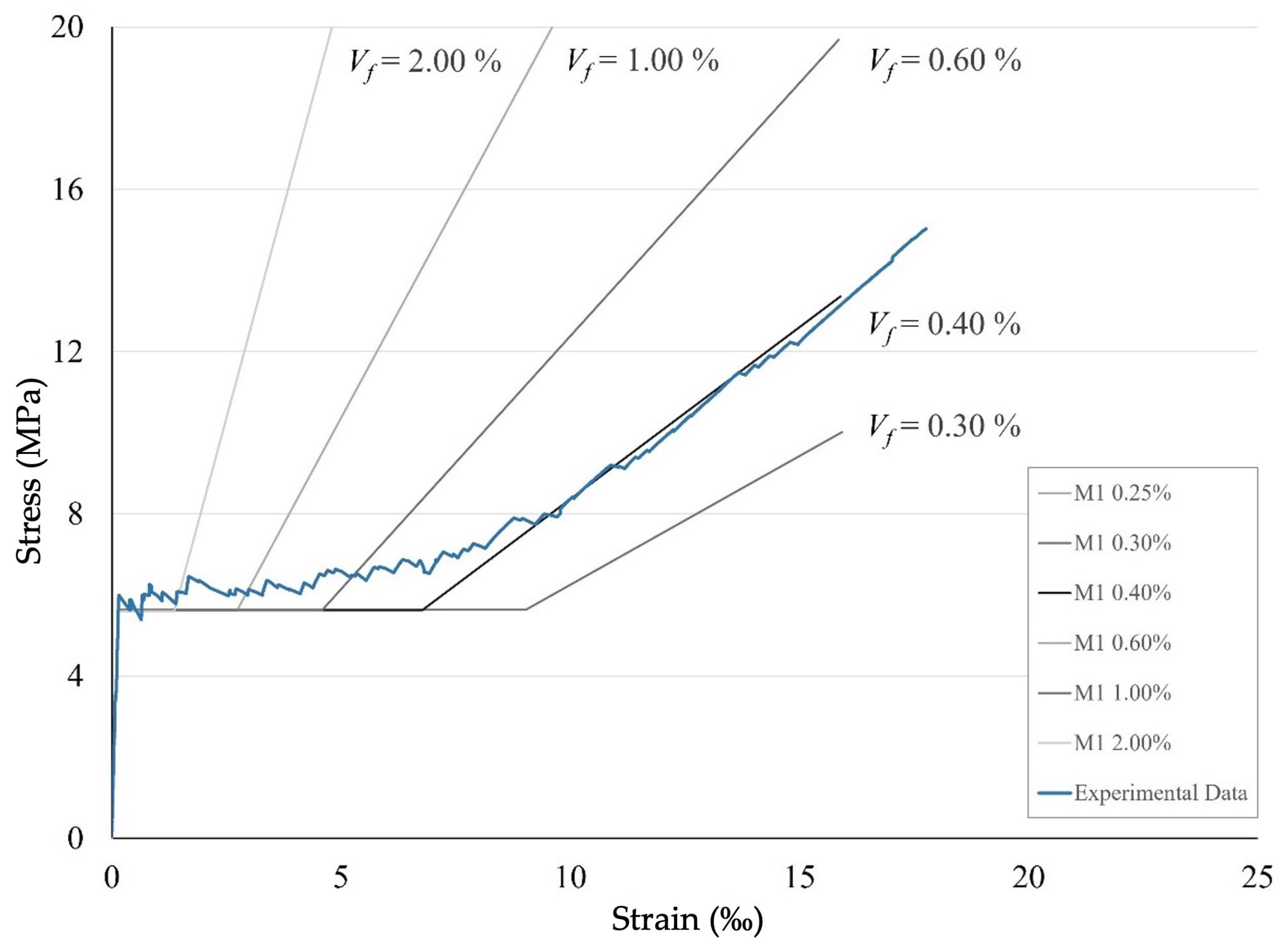
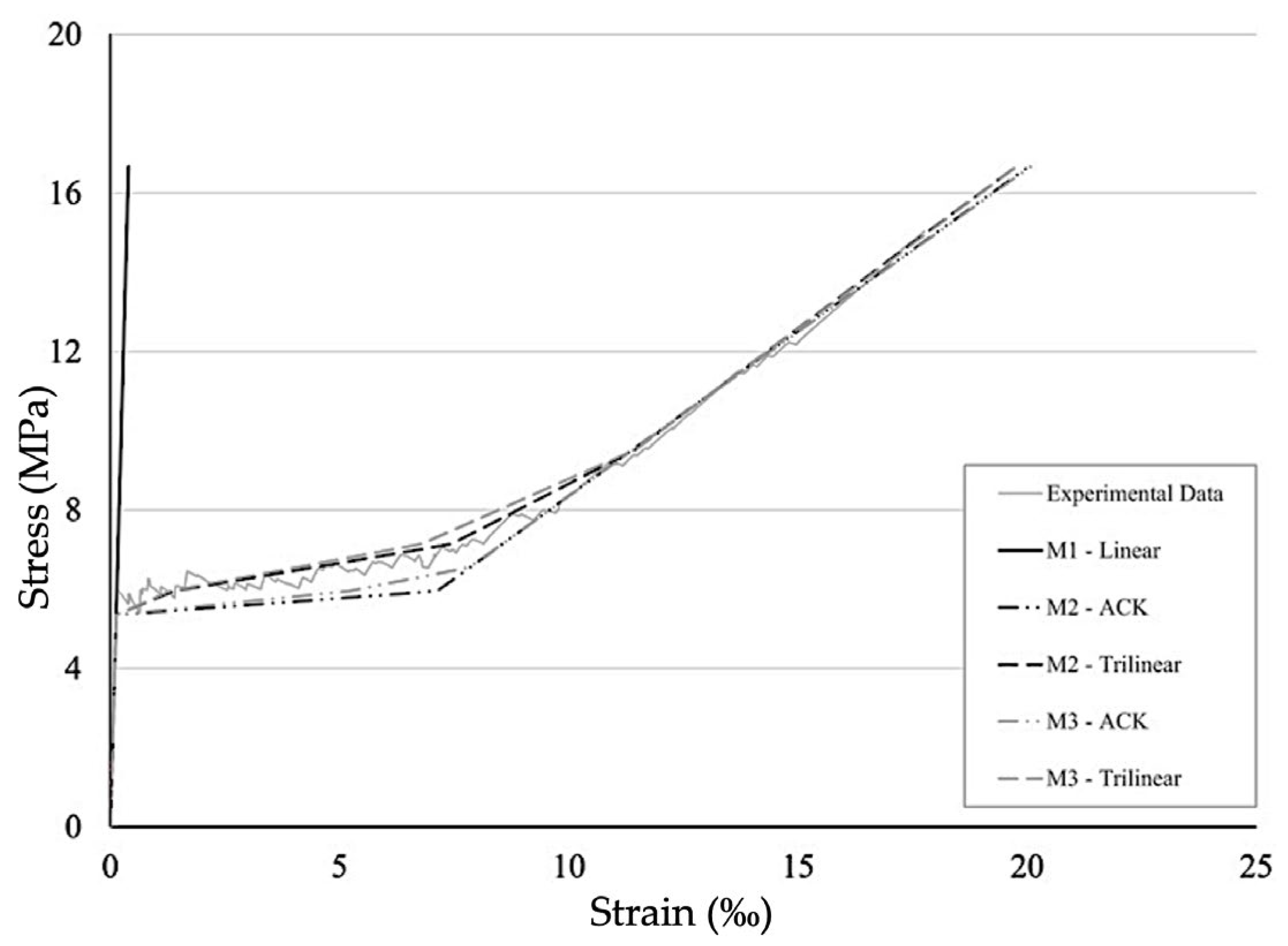
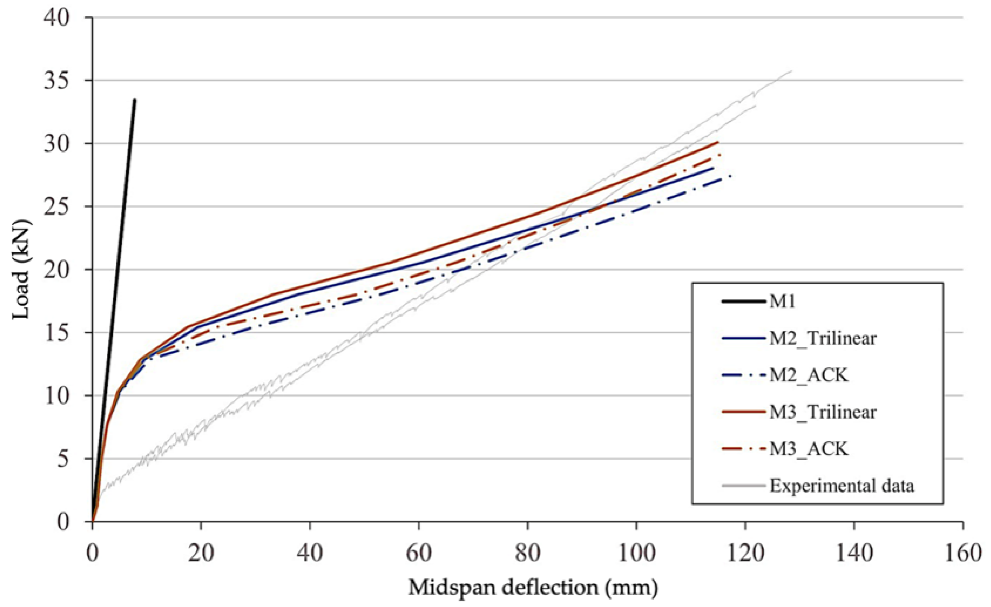
• For a broad representation of the available material models in the RFEM software package (Ver. 5.19), first, a linear elastic material model was considered, called M1 in further discussions. This approach is interesting because it reflects the material model that is considered and uses it as the preinstalled model for the calculation of concrete structures in RFEM. The CUBE project shows that such approaches can be properly used [37]. Here, the force flow over the whole structure was first simulated using the linear material model coupled with an appropriate cross-sectional stiffness. Then, for an appropriate deflection calculation, the cross-section stiffness was reduced.
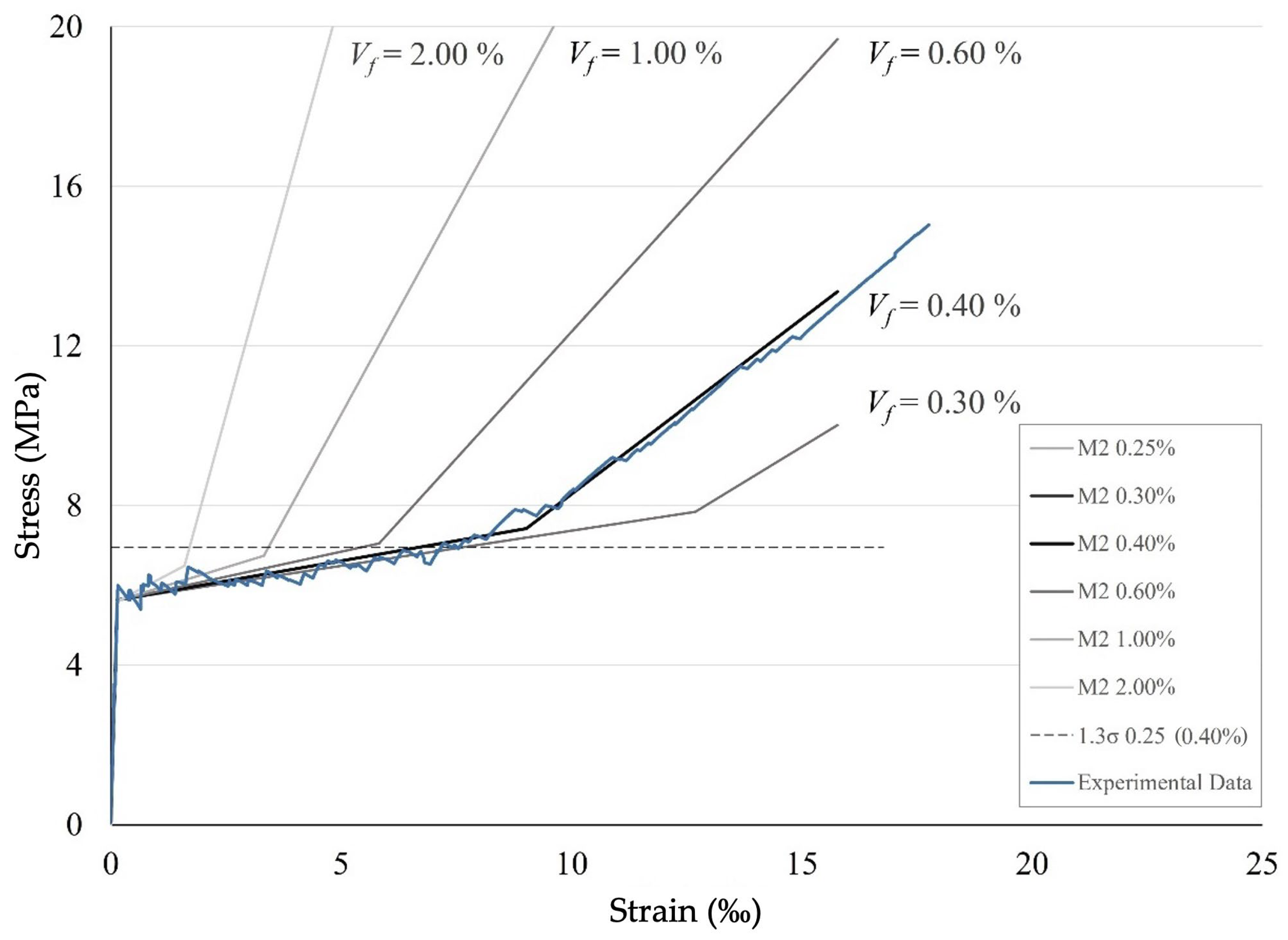
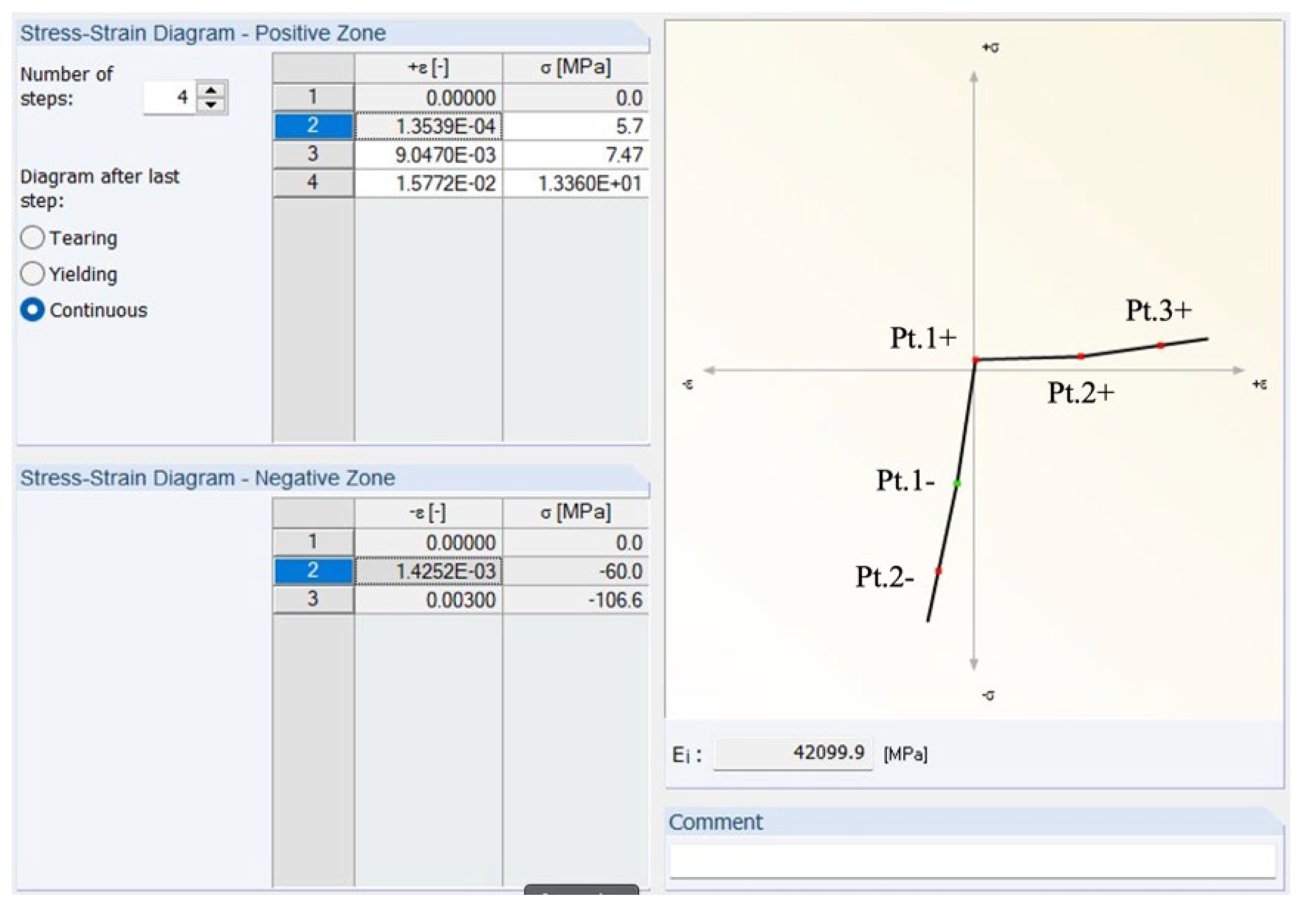
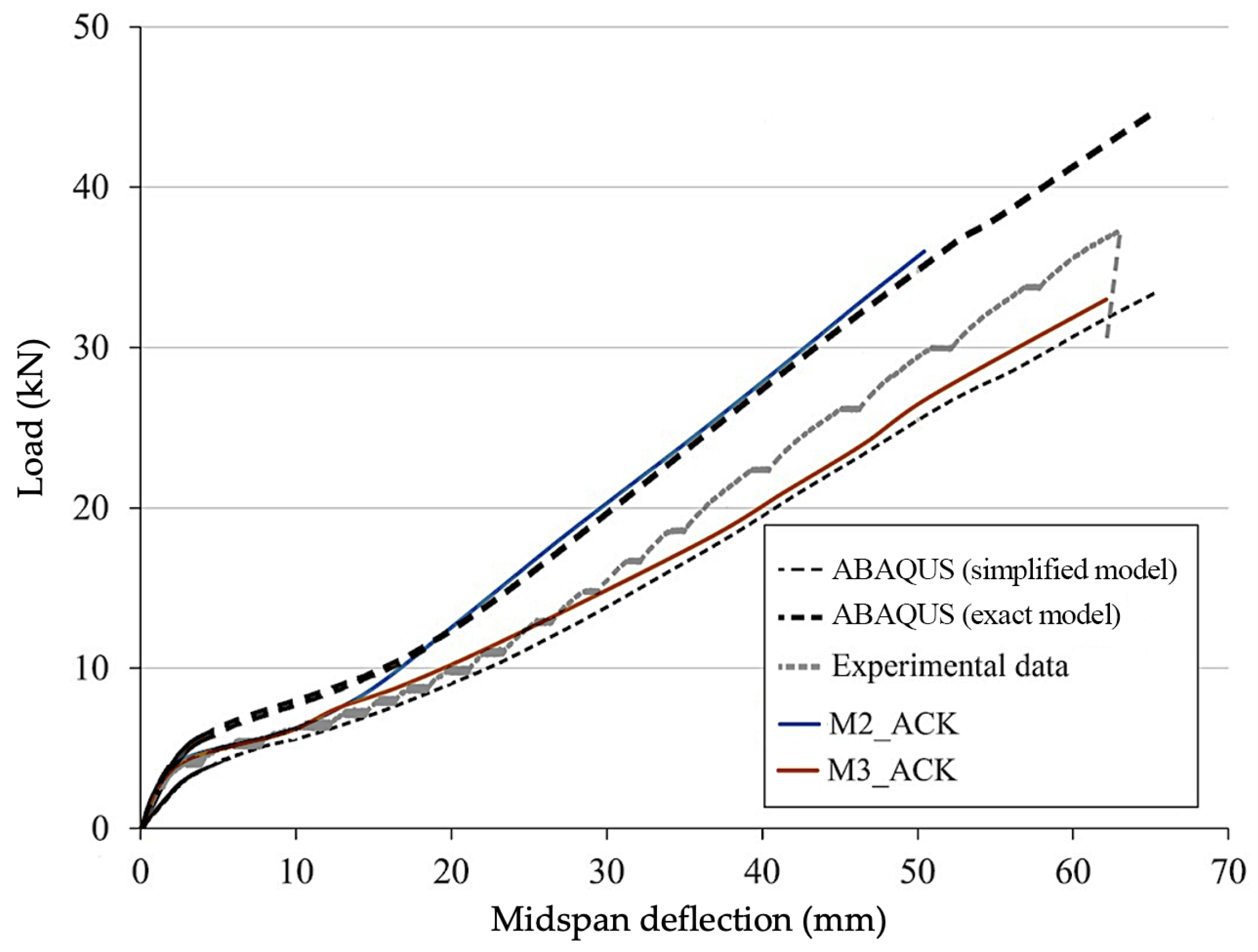
• The next material model M2 is based on M1 but it is enriched for tension with a plastic zone and a consequent strain-hardening zone. Thus, the model is able to reflect either ACK or trilinear material behaviour as described above. Within the RFEM user interface, it is possible to find an Isotropic Nonlinear Elastic 2D/3D material model which is suitable for the calculation of non-linear materials in surfaces. One of the model’s features is the possibility to provide a stress–strain curve derived from uniaxial TRC tests. A Mohr–Coulomb yield criterion is used and suitable for describing brittle materials such as concrete. The linear envelope based on the yield criteria fits for concrete with a significantly higher compressive than tensile strength. As a result, an asymmetric stress–strain diagram can be used as an input.
• The further development step regarding the material models is M3. It also gives the possibility to model TRC with nonlinear behaviour and is named in the RFEM environment as the Isotropic Damage 2D/3D model. The difference is that the model is based on the assumptions of Mazars’ damage model [38,39]. This approach provides an isotropic description of the damaged state of concrete according to [39]. The used damage function depends on scalar value D that is split into two parts, namely $D_t$ for tension and $D_c$ for compression, that can be determined from uniaxial tests. Such special features make the model attractive to be used for the calculation of TRC structures after the conduction of uniaxial tests. However, it is important to note that Mazars’ model according to the RFEM description [38] was developed for the calculation of materials with strain-softening behaviour like plain or steel fibre concrete. Thus, Mazars’ model does not fit the strain-hardening response of TRC via a smeared approach. Nevertheless, in the present study, the M3 model was used for the comparative simulation of TRC.

Figure 8 shows a stress–strain diagram of TRC within the RFEM software(Ver. 5.19) user interface which was implemented as input data for each of the above-mentioned RFEM models. For simplification, the compressive range of the concrete material selected was solved as a bilinear curve. The numerical representation of the stress–strain diagrams for ACK and trilinear models for tensile and compressive ranges is given in

Table 5. Key points of stress–strain diagram for various material models, according to Figure 8.

Diagram Points	Strain (‰)	Stress (MPa)
	ACK|Trilinear	ACK|Trilinear
Pt. 1+	0.14|0.14	5.70|5.70
Pt. 2+	6.80|9.05	5.70|7.47
Pt. 3+	15.90|15.77	13.36|13.36
Pt. 1−	0.0	−60.0
Pt. 2−	−3.0	−106.6

.

For numerical analysis stability and redundancy in the case of peak values of the applied load, the material model was defined with continuous behaviour after reaching the last point in the stress–strain diagram. To estimate the critical load, the calculations presented in Section 6 were performed stepwise. After each loading step in workflow Step II, the stress conditions were transferred to Step III for post-processing and the verification of the textile failure criteria (check Section 5).

In addition, the following RFEM software (Ver. 5.19) settings were commonly used for all calculations. The Poisson ratio $\mu$ was set as 0.2 [40]. Furthermore, the TRC shells were modelled within RFEM using 2D quadrangle elements with four nodes at corners. Degrees of freedom in nodes are displacement $\left(u_x,u_y,u_z\right)$ and rotation $\left({\phi }_x,{\phi }_y,{\phi }_z\right)$ [17]. The selected maximum FEM mesh size was 25 mm. TRC structures to be calculated were assumed to be thin walled with considerably smaller thickness than dimensions in other directions; thus, plain-stress conditions were assumed. Within RFEM, shell elements were modelled with constant thickness over the whole element. Thus, the stiffness of the elements was represented as the stiffness of a rectangular cross-section.

To initially validate the above-introduced material models within the RFEM user interface, a numerical reconstruction of the uniaxial tensile test was conducted. Figure 9 shows the resulting stress–strain diagram for the three RFEM models M1–M3 with both ACK and trilinear material models. The difference between both is especially noticeable in the state of multiple cracking (IIa). Obviously, ACK shows less stiff behaviour. The difference between the approaches used for M2 and M3 is noticeable but not significant.

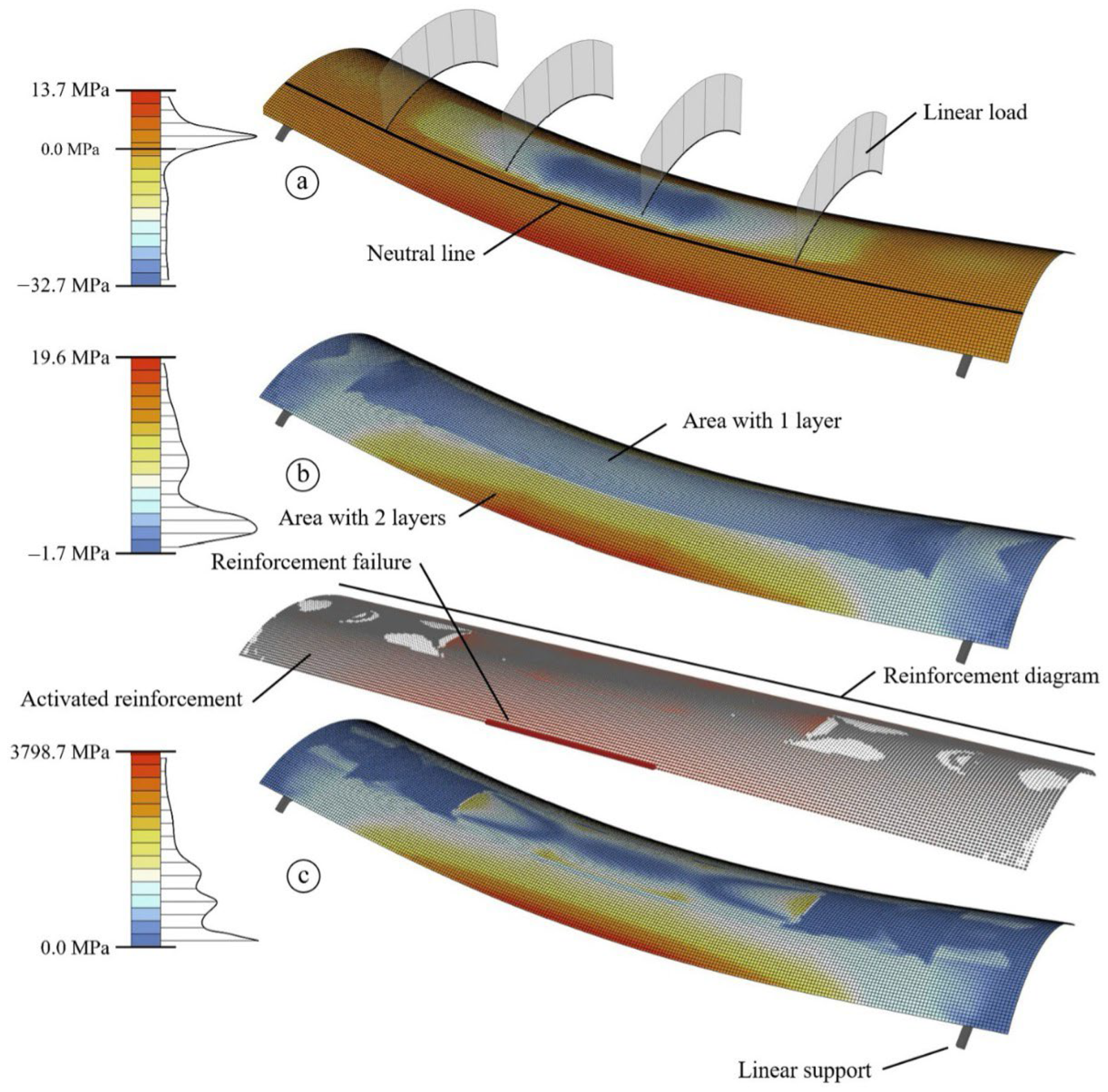
5. Textile Failure Criteria Post-Processing

To start with Step III of the workflow, the resulting values have to be exported to stand-alone Python-based scripts. For further processing, fields strain values ${\epsilon }_i^{+}\left({\phi }_j\right)$ and ${\epsilon }_i^{-}\left({\phi }_j\right)$ for the positive and negative sides of the shell elements, respectively, should be exported for each FEM node point i for two principal stress axis directions j. Thus, the FEM nodes form a set of vectors x ∈ X that defines a space X. Figure 10 shows the strain components derived from the FEM calculation.

The selected smeared material model approach possesses a significant limitation: it is impossible to correctly model the position of the reinforcement and, as a result, the inner lever arm in the case of bending. This may lead to an overestimation of stiffness in the case of significant bending [19]. It is assumed that the textile reinforcement is arranged symmetrically in the shell cross-section. Based on the central position of the reinforcement, the strain level ${\tilde{\epsilon }}_i$ of each FEM point from X for the textile reinforcement layers and corresponding in-plane tensile forces $n_{Et}\left({\phi }_j\right)$ can be estimated as follows:

$${\tilde{\epsilon }}_i=0.5·\sum \left({\epsilon }_i^{+}\left({\phi }_j\right),{\epsilon }_i^{-}\left({\phi }_j\right)\right); n_{Et,i}\left({\phi }_j\right)={\tilde{\epsilon }}_i·E_f·A_{tex} \mathrm{for} {\tilde{\epsilon }}_i\ge 0$$

(16)

where $A_{tex}$ (mm²/m) is the cross-section area of the textile reinforcement from Table 3. Such an approach gives insight into the resulting stress contained within the textile reinforcement for further comparative analysis. The resulting concrete in-plane force may be estimated according to Equation (23):

$${\sigma }_{i,Ec}\left({\phi }_j\right)=-{\int }_{{-h}_c/2}^{+h_c/2}{\epsilon }_i\left({\phi }_j,h\right)·E_{m}dh; n_{i,Ec}\left({\phi }_j\right)={\sigma }_{i,Ec}\left({\phi }_j\right)·h_c \mathrm{for} {\epsilon }_i\le 0$$

(17)

where $h_{\mathrm{c}}$ is the height of the TRC shell. After the assessment of the principal stress field, another question arises: how can we estimate the limit of the structure properly if axial forces as well as bending moments act simultaneously? A solution is the use of the n–m interaction diagram in a similar way as for steel-reinforced concrete [41]. In recent research on TRC structures, a simplified and normalized η_n–η_m interaction diagram was proposed [41,42,43]. This can be constructed using experimentally derived strength characteristics for uniaxial tension n_Rt (kN/m), uniaxial compression n_Rc (kN/m), and pure bending m_R (kNm/m), assuming a linear interpolation between them (Figure 11).

The normalized stress resultants can be calculated based on the characteristic strength values:

$${\eta }_{nt}=\frac{n_E}{n_{Rt}}; {\eta }_{nc}=-\frac{n_E}{n_{Rc}}; {\eta }_m=\frac{\left|m_E\right|}{m_R}$$

(18)

where 0 ≤ η ≤ 1.0. In the general case of combined loading, the utilization ratio η_nm can be calculated according to [41] as follows:

$${\eta }_{nm}=\mathit{max}\left({\eta }_{nt},{\eta }_{nc}\right)+{\eta }_m$$

(19)

The simplified envelope diagram shows the following characteristics [41]:

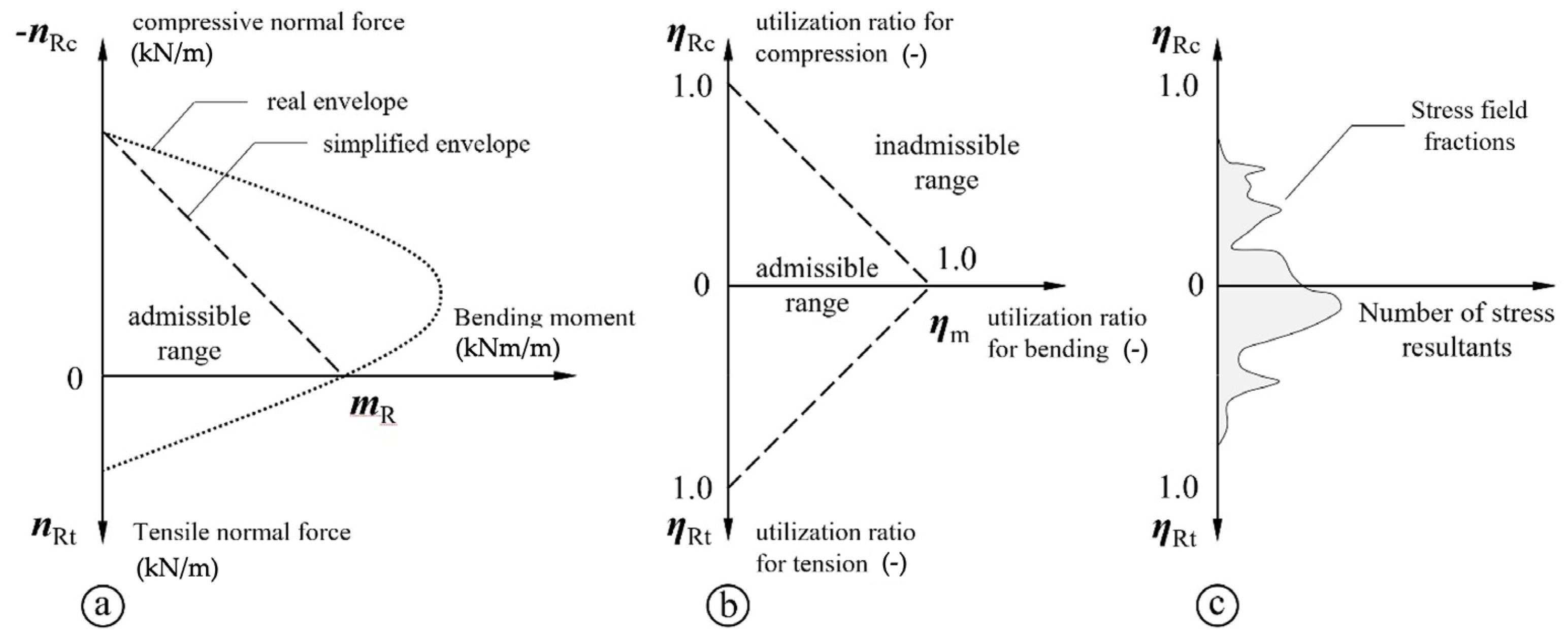
• In the tension-bending range, linear interpolation gives a relatively good representation of real behaviour.
• In the compression-bending range, the ultimate strength is underestimated by the linear interpolation, staying on the safe side.

In the first stages of the project, for simplification reasons, only in-plane actions were considered according to the general aim of the project to proceed with shell-like structures and membrane action. Therefore, the interaction diagram was modified to represent only compression and tension ranges. Figure 11c shows the modified version in the current state of the project. It contains so-called stress field fractions (SF). As a result of the estimation of the stress resultants for each FEM point x ∈ X, the points may be sorted according to their level of utilization in the range [0, 1]. The number of points in total for each level of utilization gives the diagram of SF that helps to estimate and further optimize not only the very limited critical FEM points but also points with a degree of utilization that is less than 1.0; by this, it is possible to make the TRC structure fitter according to the principle ‘form follows force’.

In the FEM calculator described in Section 4, an isotropic material model was assumed. However, the orthotropic textile reinforcement exhibits anisotropic behaviour due to the misfit between the direction of the principal stresses and the orientation of the textile yarns [43]. To account for the possible weakening factor, the design limit value for the tensile reinforcement n_t,Rd can be modified as follows [41]:

$$n_{Rt}\left(\alpha \right)=n_{Rt,0°}·\mathit{cos}\left(\alpha \right)·k_{\alpha }+n_{Rt,90°}·\mathit{sin}\left(\alpha \right)·\left(1-k_{\alpha }\right)$$

(20)

where $n_{Rt,0°}$ and $n_{Rt,90°}$ are the strengths in 0° and 90° directions, respectively. The reduction factor $k_{\alpha }$ can be calculated according to [41] via the following:

$$k_{\alpha }=1-\frac{\left|\alpha \right|}{90°}$$

(21)

Here, $\alpha$ is the deviation angle between the direction of the principal tensile stress and the orientation of the textile yarns. In the TRC shell structure presented in Section 6, the warp yarns of the textile grid are aligned in the longitudinal direction of the TRC shell and, thus, match the assumed principal stress field axis. Thus, $\alpha =0°$ and, consequently, $n_{Rt}\left(\alpha \right)=n_{Rt,0°}$. The same approach and simplification are valid for the reduction in the tensile strength due to discontinuities in the reinforcement layers [41]. This modification can be considered via a strength reduction factor that includes the number of textile layers $n_f$ and the number of interruptions $n_{f,int}$ that form an overlapping of the textile layers, as shown in the next expression:

$$k_b=\frac{n_f-n_{f,int}}{n_f}$$

(22)

For the narrow width shells that we consider in this project, it is possible to place a complete single layer over the entire structure. The reduction factor, thus, can be estimated as $k_b=1.$ To summarize, the final expressions for the calculation of normalized stress resultants, considering the above-discussed range of Equations (18)–(22), can be expressed as follows:

$${\eta }_{nc}=-\frac{n_{Ec}\left({\phi }_1\right)}{f_{cm}·h_c}$$

(23)

$${\eta }_{nt}=\frac{n_{Et}\left({\phi }_1\right)}{k_b·\mathit{cos}\left(\alpha \right)·f_{tm,tex,Q85}·A_{tex}}$$

(24)

Returning to the workflow, the failure state assessment has to be performed for each FEM node $\mathit{x}$ for either the concrete matrix in the compression range or for the reinforcement in the tensile range. Both aspects can be combined to determine the total utilization ratio according to Equation (25) and to specify the type of failure that characterizes the TRC structure [41]:

$${\eta }_{nm}^{max}\left(\mathit{x}\right)={max}_{j=1..n}\left[{\eta }_{nm,j}\left({\alpha }_j\left(\mathit{x}\right),\mathit{x}\right)\right]$$

(25)

The expression provided above has to be verified for all load cases $j$.

6. Trial-Based Calculation

To validate the material models provided above and the selected FEM procedures and to create a basis for the further development of the workflow, an arch-like shell was selected to perform a bending test according to the reference project [44], Figure 12. The total length of the shell is 2700 mm and the width is 600 mm. The shell provided has articulated linear supports from both ends in longitudinal direction of the shell. The clear span between the supports is 2500 mm. The transversal profile follows a chain line with a rise in the shell in the middle point of 100 mm. Due to manufacturing constraints, the thickness of the shell was set to be 40 mm. Prior to the experiments, the TRC shell was simulated; in the first step, it was simulated only with one single main layer of the solidian GRID Q85-CCE-21-E5 completely over the whole element. The loading was selected according to EN 1991-1-1 [45] for residential use, comprising a 2.0 kN/m² area load and a 3.0 kN point load. In the ultimate limit state, the textile stresses in the tension zone were higher than the design value for the textile. Therefore, it was decided to place two 200 mm wide additional textile stripes symmetrically in the tensile zone of the shell (Figure 12). The textile layers were arranged analogously to the uniaxial tensile samples with 10 mm spacing between the layers and a 15 mm concrete cover.

For the validation of the numerical model, laboratory experiments with simulated TRC shells were performed. According to the technical constraints of the lab, the initial area load was converted into four equal line loads (see Figure 13a), resulting in a six-point bending test. The load was introduced in a displacement-controlled manner with a velocity of 0.05 mm/s until failure. In total, two shells were tested. Figure 13 gives the results for the limit stress state that corresponds to 12.1 kN/m for each line load or a total of 31 kN of an accumulated load.

Figure 13a,b show the stress state of the composite, where ${\sigma }_i^{+}$ stands for the top and ${\sigma }_i^{-}$ stands for the bottom side of the shell. As may be seen from the legends, the compression zone lies between the top and bottom sides of the shell. Consequently, the TRC shell possesses significant bending action that is in contradiction with the accepted calculation hypothesis. The maximum stress of the concrete matrix reaches a magnitude of –32.7 MPa. That magnitude corresponds to only 28.5% of the experimentally determined concrete strength of $f_{cm}=$ 114.8 MPa. Thus, it is expected that a reinforcement failure will be obtained during the experiment. Additionally, this result indicates that there is still a relatively large potential for material optimization that may reduce the compression zone and increase the utilization ratio of the concrete under compression. The reinforcement diagram in Figure 13c shows that in the middle section of the shell, the magnitude of ${\tilde{\epsilon }}_i>0$, and consequently, the reinforcement is considered to be activated. In the critical tensile zone of the shell, two layers of reinforcement reach the limit of $f_{tm,tex,Q85}=$ 3750.0 MPa. The textile tensile strength magnitude was directly calculated from the mean value of composite strength from the conducted uniaxial tensile experiments (Figure 6 and Figure 7). It can be calculated with a modified Equation (7) as follows:

$$f_{tm,tex,Q85}=\frac{{\tilde{\sigma }}_{cu}}{V_f}$$

(26)

where $V_f$ = 0.4% and ${\tilde{\sigma }}_{cu}$ = 15 MPa (composite’s ultimate strength). In the bending tests, we detected midpoint deflections between 121.9 and 128.6 mm and reached failure loads between 33.0 and 35.7 kN, resulting in averages of 125.3 mm and 34.4 kN. The failure load according to the textile failure estimation procedure described above, derived at levels of 27.8 kN and 29.7 kN for the material models M2 and M3, respectively.

Figure 14 reflects the midspan deflections derived from tested shells and deflection results obtained from numerical analysis using the first linear model, M1, as a reference and the two different models described above, M2 and M3, with variations provided by input data from trilinear and ACK material models.

As expected, the linear model M1 gives good agreement only in the uncracked state. In general, all models show deficits in State II. Furthermore, there is a clear influence of the input data developed according to the trilinear and ACK material models. The ACK approach (M2) gives slightly less stiffness behaviour than the M3 material model, which matches the experimental data at the end of test a bit better. In general, the overestimation of the stiffness may be a cumulative result of various reasons. Nevertheless, one of the key results is that the smeared model does not give a correct bending load response at the first stages of loading history due to weak behaviour for non-membrane actions, regardless of the utilized material model. In more details such effects were studied in [19]. Accordingly, all the evaluated layers that the cross-section of the shell can be subdivided in over the height follow the same strain-hardening curve. The stress profile was calculated from the strain level distribution. As a result, all the layers of the composite material contribute to the bending stiffness with the corresponding lever arm, even from the areas where the concrete is cracked. Consequently, it is not possible to reflect the effect of the position of the textile reinforcement in the cross-section; in turn, it is impossible to represent the effect of the reinforcement lever arm.

The discussion and consequent hypothesis regarding a possible reason for the overestimation of the structural stiffness of the tested shell-like structures need to be strengthened. For this purpose, experiments carried out earlier at our institute in another project were used as alternative shell structures (Figure 15); more details arme described in [19,44].

The main shell thickness was 1 cm with minor differences in the middle area of the shell element. The neutral line was located approx. 50 mm from the shell’s vertex [44]. Therefore, it may be indicated that the top and bottom parts of the shell possess mainly membrane forces, in contrast to the previously presented shells with a neutral line inside the element’s thickness. For comparison purposes, the alternative shell was modelled in RFEM software (Ver. 5.19) using the M2 and M3 material models. The stress–strain relations for the models are based on uniaxial tests on the used textiles [19] according to ACK methodology. The key points of the stress–strain diagrams are provided in

Table 6. Key points of stress–strain diagrams in RFEM software (Ver. 5.19) for positive range of the material behaviour.

Diagram Points	Strain (‰)	Stress (MPa)
	3300 tex|3300 + 800 tex	3300 tex|3300 + 800 tex
Pt. 1+	0.086|0.086	2.40|2.40
Pt. 2+	2.00|1.40	2.40|2.40
Pt. 3+	7.20|7.30	19.00|30.00

.

In Figure 16, in addition to test values, force–midspan deflection curves from calculations using M2 and M3 models in RFEM are shown, as well as curves derived with a smeared approach using the ABAQUS (Ver. 6.10) software package for simplified model with 10 mm shell thick and exact model according to the design [19]. It can be seen from the figure that the models M2 and M3 give good agreement with the reference smeared approach calculation and the experimental results. This agreement supports the hypothesis that the smeared TRC calculation approach can be used in RFEM for structures with predominantly membrane actions. It is also important to note that model M3 with Mazars’ hypothesis provides good agreement, even though the TRC material behaves in a strain-hardening manner.

7. Conclusions

First, for this project, the numerical analysis workflow was assembled, and it shows a reasonable response. There is still a list of components to be upgraded, like, in general, the numerical analysis type and failure criteria assessment routines. However, the basic components show a good background for the further development of analysis routines and enable us to switch now to the multi-objective optimization of TRC shell structures. Second, we show that the RFEM (Ver. 5.19) software package as a FEM solver can be used for the calculation of thin-walled TRC structures according to a smeared approach, with pre-installed material models and proper calibration based on uniaxial tests. From the results, it follows that such an application provides a better fit for TRC structures with a membrane-dominant behaviour. The influence of the bending action may potentially lead to a significant overestimation of the structural stiffness of TRC structures, as it was calculated by the verification of the deflection behaviour of the original arch-like shell. The derived results from comparable research between both shell geometries legitimate the need for further research within the scope of the project, such as the conversion of the numerical model to the resolved layer approach, mentioned earlier in this paper, to expand the functionality of the proposed workflow for TRC structures with significant bending action. In that way, the TRC structures can be presented as multilayer systems with one layer representing the concrete matrix in the shell and the other representing the textile. It will provide more appropriate data for the M3 Mazars damage model calibrated for brittle-like materials.

A comprehensive numerical parameter study is currently being carried out in this project. The aim is to determine under what conditions and to what extend a shell load-bearing effect can occur inside a component and what influence, for example, geometrical topology and boundary conditions, imperfections, and material properties have. Selected laboratory tests will serve to verify the model.

References

1. Bologna, A.; Gargiani, R. The Rhetoric of Pier Luigi Nervi: Forms in Reinforced Concrete and Ferrocement; EPFL Presses: Lausanne, Switzerland, 2016. [Google Scholar]
2. Mata-Falcon, J.; Bischof, P.; Huber, T.; Anton, A.; Burger, J.; Ranaudo, F.; Jipa, A.; Gebhard, L.; Reiter, L.; Lloret-Fritschi, E.; et al. Digitally Fabricated Ribbed Concrete Floor Slabs: A Sustainable Solution for Construction. RILEM Tech. Lett. 2022, 7, 68–78. [Google Scholar] [CrossRef]
3. Frenzel, M.; Farwig, K.; Curbach, M. Leichte Deckentragwerke aus geschichteten Hochleistungsbetonen | Lightweight Ceiling Structures Made of Layered High-Performance Concrete. In SPP 1542: Leicht Bauen mit Beton. Grundlagen für das Bauen der Zukunft mit Bionischen und Mathematischen Entwurfsprinzipien (Abschlussbericht)|SPP 1542: Concrete Light. Future Concrete Structures Using Bionic, Mathematical and Engineering Formfinding Principles (Final Report); Scheerer, S., Curbach, M., Eds.; Institut für Massivbau der TU Dresden: Dresden, Germany, 2022; pp. 144–169. [Google Scholar] [CrossRef]
4. Cuypers, H.; Wastiels, J. Analysis and Verification of the Performance of Sandwich Panels with Textile Reinforced Concrete Faces. J. Sandw. Struct. Mater. 2011, 13, 589–603. [Google Scholar] [CrossRef]
5. Frenzel, M. Zum Tragverhalten von Leichten, Geschichteten Betondecken. Ph.D. Dissertation, Technischen Universität Dresden, Dresden, Germany, 2021. Available online: https://nbn-resolving.org/urn:nbn:de:bsz:14-qucosa2-787009 (accessed on 9 December 2023).
6. Williams Portal, N.; Flansbjer, M.; Zandi, K.; Wlasak, L.; Malaga, K. Bending Behaviour of Novel Textile Reinforced Concrete-foamed Concrete (TRC-FC) Sandwich Elements. Compos. Struct. 2017, 177, 104–118. [Google Scholar] [CrossRef]
7. Schmeer, D.; Sobek, W. Gradientenbeton. In Beton-Kalender 2019; Bergmeister, K., Fingerloos, F., Wörner, J.-D., Eds.; Ernst & Sohn: Berlin, Germany, 2019; pp. 455–476. [Google Scholar] [CrossRef]
8. Schmeer, D.; Wörner, M.; Garrecht, K.; Sawodny, O.; Sobek, W. Effiziente automatisierte Herstellung multifunktional gradierter Bauteile mit mineralischen Hohlkörpern|Efficient Automated Production of Multifunctional Graded Components with Mineral Hollow Bodies. In SPP 1542: Leicht Bauen mit Beton. Grundlagen für das Bauen der Zukunft mit Bionischen und Mathematischen Entwurfsprinzipien (Abschlussbericht)|SPP 1542: Concrete Light. Future Concrete Structures Using Bionic, Mathematical and Engineering Formfinding Principles (Final Report); Scheerer, S., Curbach, M., Eds.; Institut für Massivbau der TU Dresden: Dresden, Germany, 2022; pp. 250–282. [Google Scholar] [CrossRef]
9. Beckmann, B.; Bielak, J.; Bosbach, S.; Scheerer, S.; Schmidt, C.; Hegger, J.; Curbach, M. Collaborative Research on Carbon Reinforced Concrete Structures in the CRC/TRR 280 Project. Civ. Eng. Des. 2021, 3, 99–109. [Google Scholar] [CrossRef]
10. Main Website of Collaborative Research Centre/Transregio 280, (CRC/TRR 280). Available online: https://www.sfbtrr280.de/en/ (accessed on 9 December 2023).
11. Hegger, J.; Curbach, M.; Stark, A.; Wilhelm, S.; Farwig, K. Innovative Design Concepts: Application of Textile Reinforced Concrete to Shell Structures. Struct. Concr. 2018, 19, 637–646. [Google Scholar] [CrossRef]
12. McNeel Europe SL, Rhinoceros 3D, Version 7.0. Available online: https://www.rhino3d.com/ (accessed on 9 December 2023).
13. Robert McNeel & Associates, Grasshopper 3D, Version 7.0. Available online: https://www.grasshopper3d.com/ (accessed on 9 December 2023).
14. RF-COM/RS-COM Add-on Module for RFEM/RSTAB. Available online: https://www.dlubal.com/en/products/rfem-and-rstab-add-on-modules/others/rf-com (accessed on 9 December 2023).
15. Vakaliuk, I.; Frenzel, M.; Curbach, M. Application of Parametric Design Tools for the Roof of the C3 Technology Demonstration House—CUBE. In Form and Force—Proceedings of the IASS Annual Symp. 2019/Structural Membranes 2019; Lázaro, C., Bletzinger, K.-U., Oñate, E., Eds.; International Centre for Numerical Methods in Engineering (CIMNE): Barcelona, Spain, 2019; pp. 1077–1084. [Google Scholar]
16. Koschemann, M.; Vakaliuk, I.; Curbach, M. An Ultra-Light Carbon Concrete Bridge: From Design to Realisation. In Proceedings of the Concrete Innovation for Sustainability—Proceedings for the 6th fib International Congress 2022, Oslo, Norway, 12–16 June 2022; Stokkeland, S., Braarud, H.C., Eds.; Novus Press: Oslo, Norway, 2022; pp. 2458–2467. [Google Scholar]
17. Dlubal Software GmbH, RFEM, Version 5.19. Available online: www.dlubal.com (accessed on 9 December 2023).
18. Vakaliuk, I.; Platen, J.; Klempt, V.; Scheerer, S.; Curbach, M.; Kaliske, M.; Löhnert, S. Development of Load-Bearing Shell-Type TRC Structures—Initial Numerical Analysis. In Proceedings of the Concrete Innovation for Sustainability—Proceedings for the 6th fib International Congress 2022, Oslo, Norway, 12–16 June 2022; Stokkeland, S., Braarud, H.C., Eds.; Novus Press: Oslo, Norway, 2022; pp. 1235–1244. [Google Scholar]
19. Chudoba, R.; Sharei, E.; Senckiel-Peters, T.; Schladitz, F. Numerical Modelling of Non-Uniformly Reinforced Carbon Concrete Lightweight Ceiling Elements. Appl. Sci. 2019, 9, 2348. [Google Scholar] [CrossRef]
20. Jesse, F. Tragverhalten von Filamentgarnen in Zementgebundener Matrix. Ph.D. Dissertation, Technische Universität Dresden, Dresden, Germany, 2005. Available online: https://nbn-resolving.org/urn:nbn:de:swb:14-1122970324369-39398 (accessed on 2 March 2024).
21. Hartig, J. Numerical Investigations on the Uniaxial Tensile Behaviour of Textile Reinforced Concrete. Ph.D. Dissertation, Technische Universität Dresden, Dresden, Germany, 2011. [Google Scholar]
22. Bentur, A.; Mindess, S. Fibre Reinforced Cementitious Composites; Modern Concrete Technology Series; E & FN Spon: London, UK, 1990; ISBN 0–415–25048–X (hbk). [Google Scholar]
23. Nathan, G.K.; Paramasivam, P.; Lee, S.L. Tensile Behaviour of Fiber Reinforced Cement Paste. J. Ferrocem. 1977, 7, 59–79. [Google Scholar]
24. Telford, T. CEB-FIP Model Code 1990: Design Code; Thomas Telford Services Ltd., Thomas Telford House: London, UK, 1993. [Google Scholar]
25. Blom, J.; Wastiels, J. Modelling Textile Reinforced Cementitious Composites—Effect of Elevated Temperatures. In Proceedings of the 19th International Conference on Composite Materials, Montreal, QC, Canada, 28 July–2 August 2013; pp. 7098–7108. [Google Scholar]
26. Blom, J.; Cuypers, H.; Van Itterbeeck, P.; Wastiels, J. Modelling the Behaviour of Textile Reinforced Cementitious Composites under Bending. In Proceedings of the Fibre Concrete 2007 Technology, Design, Application, Prague, Czech Republic, 12–13 September 2007; pp. 205–210. [Google Scholar]
27. Jesse, F.; Ortlepp, R.; Curbach, M. Tensile Stress-Strain Behaviour of Textile Reinforced Concrete. In Proceedings of the towards a Better Built Environment—Inovation, Sustainability, Information Technology—Proceedings of the IABSE Symp, Melbourne, Australia, 11–13 September 2002; Volume 86, pp. 376–377. [Google Scholar]
28. Zilch, K.; Zehetmaier, G. Bemessung im konstruktiven Betonbau: Nach DIN 1045-1 und EN 1992-1-1, 2nd ed.; Springer: Berlin/Heidelberg, Germany, 2010; ISBN 978-3-540-70637-3. [Google Scholar]
29. Ng, H.K.; Nathan, G.K.; Paramasivam, P.; Lee, S.L. Tensile Properties of Steel Fiber Reinforced Mortar. J. Ferrocem. 1978, 8, 219–229. [Google Scholar]
30. Carbon Concrete Composite [Homepage]. Available online: https://www.bauen-neu-denken.de/en/ (accessed on 9 December 2023).
31. Wilhelm, K. Verbundverhalten von Mineralisch und Polymer Gebundenen Carbonbewehrungen und Beton bei Raumtemperatur und erhöhten Temperaturen bis 500 °C. Ph.D. Dissertation, Technische Universität Dresden, Dresden, Germany, 2021. Available online: https://nbn-resolving.org/urn:nbn:de:bsz:14-qucosa2-770999 (accessed on 9 December 2023).
32. DIN EN 196-1:2016-11; Prüfverfahren für Zement—Teil 1: Bestimmung der Festigkeit. Beuth Verlag: Berlin, Germany, 2016.
33. Technical Data Sheet Solidian GRID Q85-CCE-21-E5. 2023. Available online: https://solidian.com/wp-content/uploads/solidian-GRID-Qxx-CCE-xx-Technical-Product-Data-Sheets-v2402.pdf (accessed on 9 December 2023).
34. Vakaliuk, I.; Scheerer, S.; Curbach, M. Initial Laboratory Test of Load-Bearing Shell-Shaped TRC Structures. In Concrete Innovation for Sustainability, Proceedings of the 6th fib International Congress, Oslo, Norway, 12–16 June 2022; Stokkeland, S., Braarud, H.C., Eds.; Novus Press: Oslo, Norway, 2022; pp. 675–684. [Google Scholar]
35. Schütze, E.; Bielak, J.; Scheerer, S.; Hegger, J.; Curbach, M. Einaxialer Zugversuch für Carbonbeton mit textiler Bewehrung | Uniaxial Tensile Test for Carbon Reinforced Concrete with Textile Reinforcement. Beton Stahlbetonbau 2018, 113, 33–47. [Google Scholar] [CrossRef]
36. Rempel, S. Zur Zuverlässigkeit der Bemessung von Biegebeanspruchten Betonbauteilen mit textiler Bewehrung. Ph.D. Dissertation, RWTH Aachen, Aachen, Germany, 2018. [Google Scholar] [CrossRef]
37. Zavadski, V.; Frenzel, M. Aufbau, Bemessung und Planung der TWIST-Carbonbetonschalen. Beton Stahlbetonbau 2023, 118, 71–81. [Google Scholar] [CrossRef]
38. Mazars, J.; Grange, S. Simplified Strategies Based on Damage Mechanics for Concrete under Dynamic Loading. Philos. Trans. R. Soc. A 2017, 375, 20160170. [Google Scholar] [CrossRef]
39. Mazars, J. A Description of Micro- and Macroscale Damage of Concrete Structures. Eng. Fract. Mech. 1986, 25, 729–737. [Google Scholar] [CrossRef]
40. Sharei, E. Simulation Concepts for Concrete Structures with Discrete and Smeared Representation of Reinforcement. Ph.D. Dissertation, RWTH Aachen, Aachen, Germany, 2018. [Google Scholar]
41. Scholzen, A.; Chudoba, R.; Hegger, J. Thin-Walled Shell Structures Made of Textile-Reinforced Concrete. Struct. Concr. 2015, 16, 115–124. [Google Scholar] [CrossRef]
42. Sharei, E.; Chudoba, R.; Scholzen, A. Cross-Sectional Failure Criterion Combined with Strain-Hardening Damage Model for Simulation of Thin-Walled Textile-Reinforced Concrete Shells. In Proceedings of the in ECCOMAS Congress 2016 VII European Congress on Computational Methods in Applied Sciences and Engineering; Papadrakakis, M., Papadopoulos, V., Stefanou, G., Plevris, V., Eds.; Institute of Structural Analysis and Antiseismic Research School of Civil Engineering National Technical University Athens: Crete Island, Greece, 2016; pp. 6823–6831. [Google Scholar]
43. Scholzen, A.; Chudoba, R.; Hegger, J. Ultimate Limit State Assessment of TRC Shell Structures with Combined Normal and Bending Loading. In Proceedings of the 11th International Symposium on Ferrocement and Textile Reinforced Concrete, Aachen, Germany, 7–10 June 2015; RILEM Publ.: Bagneux, France, 2015; pp. 159–166. [Google Scholar]
44. Senckpiel, T.; Häussler-Combe, U. Experimental and Computational Investigations on Shell Structures Made of Carbon Reinforced Concrete. In Proceedings of the Interfaces: Architecture, Engineering, Science—Proceedings of Annual Meeting of the International Association of Shell & Spatial Structures (IASS), Hamburg, Germany, 25–27 September 2017; pp. 1–8. [Google Scholar]
45. EN 1991-1-1; Eurocode 1: Actions on Structures—Part 1-1: General Actions—Densities, Self-Weight, Imposed Loads for Buildings. 2002. Available online: https://www.phd.eng.br/wp-content/uploads/2015/12/en.1991.1.1.2002.pdf (accessed on 9 December 2023).
Figure 1. Overview of the workflow. Graphic: Iurii Vakaliuk.
Applsci 14 02140 g001
Figure 2. Classification of modelling approaches of textile reinforced concrete under tension including the stress–strain relations in the cross-section. Graphic: Rostislav Chudoba, see [19].
Applsci 14 02140 g002
Figure 3. Principal behaviour of the ACK material model. Graphic: Iurii Vakaliuk.
Applsci 14 02140 g003
Figure 4. Principle of the trilinear material model. Graphic: Iurii Vakaliuk.
Applsci 14 02140 g004
Figure 5. Tensile tests on TRC; (a) sample geometry, (b) sample during testing. Graphic: Silke Scheerer; photo: Iurii Vakaliuk.
Applsci 14 02140 g005
Figure 6. Calibrated ACK material model for various values of volume fraction V f . Graphic: Iurii Vakaliuk.
Applsci 14 02140 g006
Figure 7. Calibrated trilinear material model for various values of volume fraction V f . Graphic: Iurii Vakaliuk.
Applsci 14 02140 g007
Figure 8. RFEM user interface with implemented stress–strain diagram. Graphic: Iurii Vakaliuk.
Applsci 14 02140 g008
Figure 9. Reconstructed uniaxial tests in RFEM using various material models. Graphic: Iurii Vakaliuk.
Applsci 14 02140 g009
Figure 10. The shell strain and stress state. Graphic: Iurii Vakaliuk.
Applsci 14 02140 g010
Figure 11. Interaction diagrams proposed for TRC shell structures; (a) n–m initial diagram; (b) ηn–ηm simplified and normalized diagram [41,43]; (c) modified interaction diagram considering the calculation strategy of the project.
Applsci 14 02140 g011
Figure 12. General view of the TRC shell for the trial-based calculation. Graphic: Iurii Vakaliuk.
Applsci 14 02140 g012
Figure 13. Composite stress state field of the shell according to an accumulated load of 31.0 kN; (a) shell’s top side σ i + ; (b) bottom side of the shell σ i ; (c) textile reinforcement stress field. Graphic: Iurii Vakaliuk.
Applsci 14 02140 g013
Figure 14. Force–midspan deflection relationships determined in the lab tests and in simulations by using M1–M3 material models. Graphic: Iurii Vakaliuk.
Applsci 14 02140 g014
Figure 15. Alternative TRC shell structure. Graphic: Iurii Vakaliuk based on [19,45].
Applsci 14 02140 g015
Figure 16. Experimental and calculated force–midspan deflection curves for the alternative TRC shell from [19]. Graphic: Ehsan Sharei and Iurii Vakaliuk.
Applsci 14 02140 g016