Author Contributions
Conceptualization, W.L. and Y.K.; methodology, W.L.; software, W.L.; validation, W.L.; formal analysis, W.L.; investigation, W.L.; data curation, W.L.; writing—original draft preparation, W.L.; writing—review and editing, W.L. and Y.K.; visualization, W.L.; supervision, Y.K.; project administration, Y.K.; funding acquisition, Y.K. All authors have read and agreed to the published version of the manuscript.
Figure 1.
Progression of convolutional operations from the initial to the deeper layer in U-Net [
15].
Figure 1.
Progression of convolutional operations from the initial to the deeper layer in U-Net [
15].
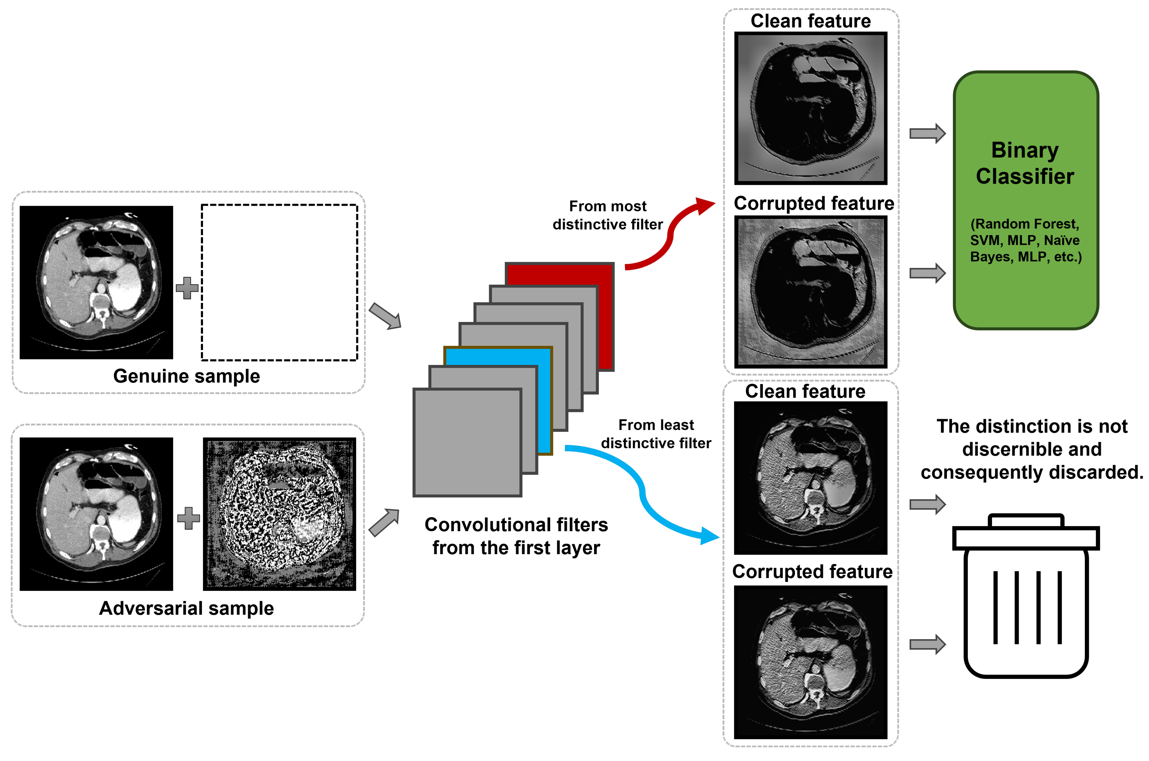
Figure 2.
Core mechanism of the proposed approach contrasting genuine and adversarial feature responses.
Figure 2.
Core mechanism of the proposed approach contrasting genuine and adversarial feature responses.
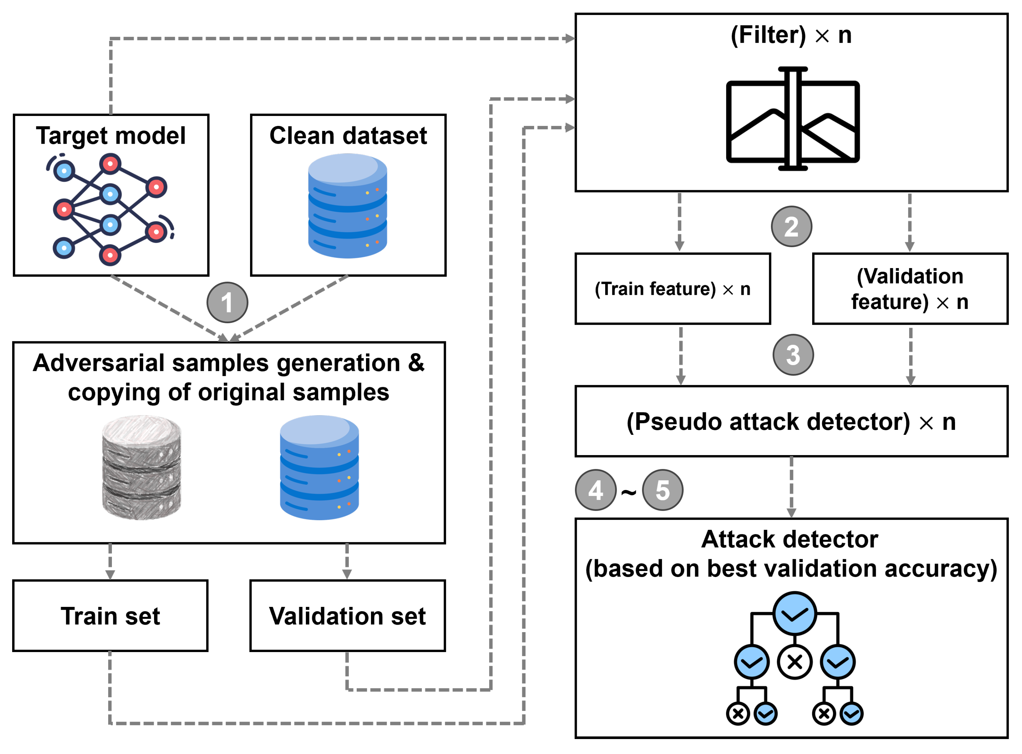
Figure 3.
Schematic representation of the attack detector derivation using the proposed approach.
Figure 3.
Schematic representation of the attack detector derivation using the proposed approach.
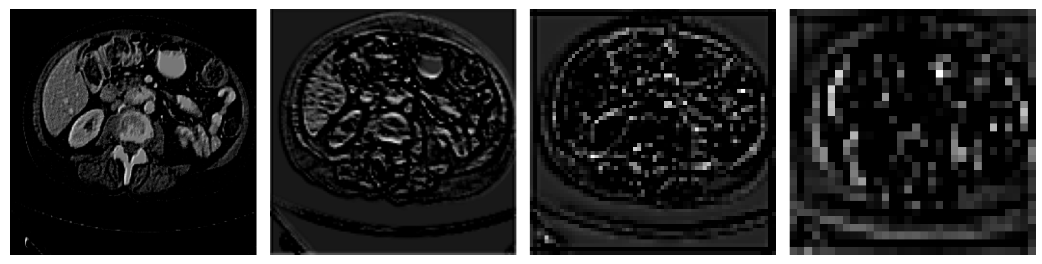
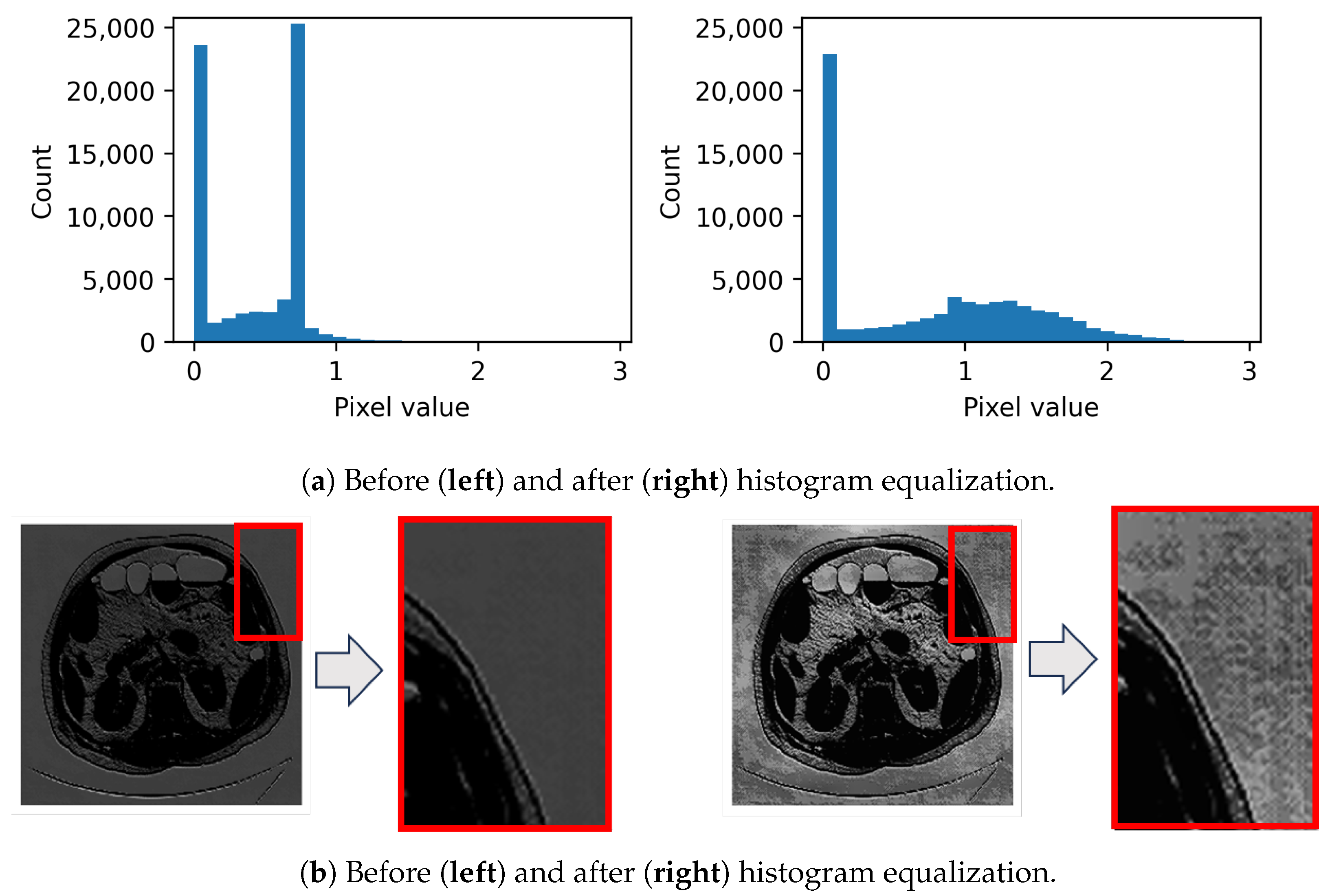
Figure 4.
Amplification of feature values via histogram equalization for enhanced perturbation visualization of a specific feature: (a) Histograms and corresponding (b) images.
Figure 4.
Amplification of feature values via histogram equalization for enhanced perturbation visualization of a specific feature: (a) Histograms and corresponding (b) images.
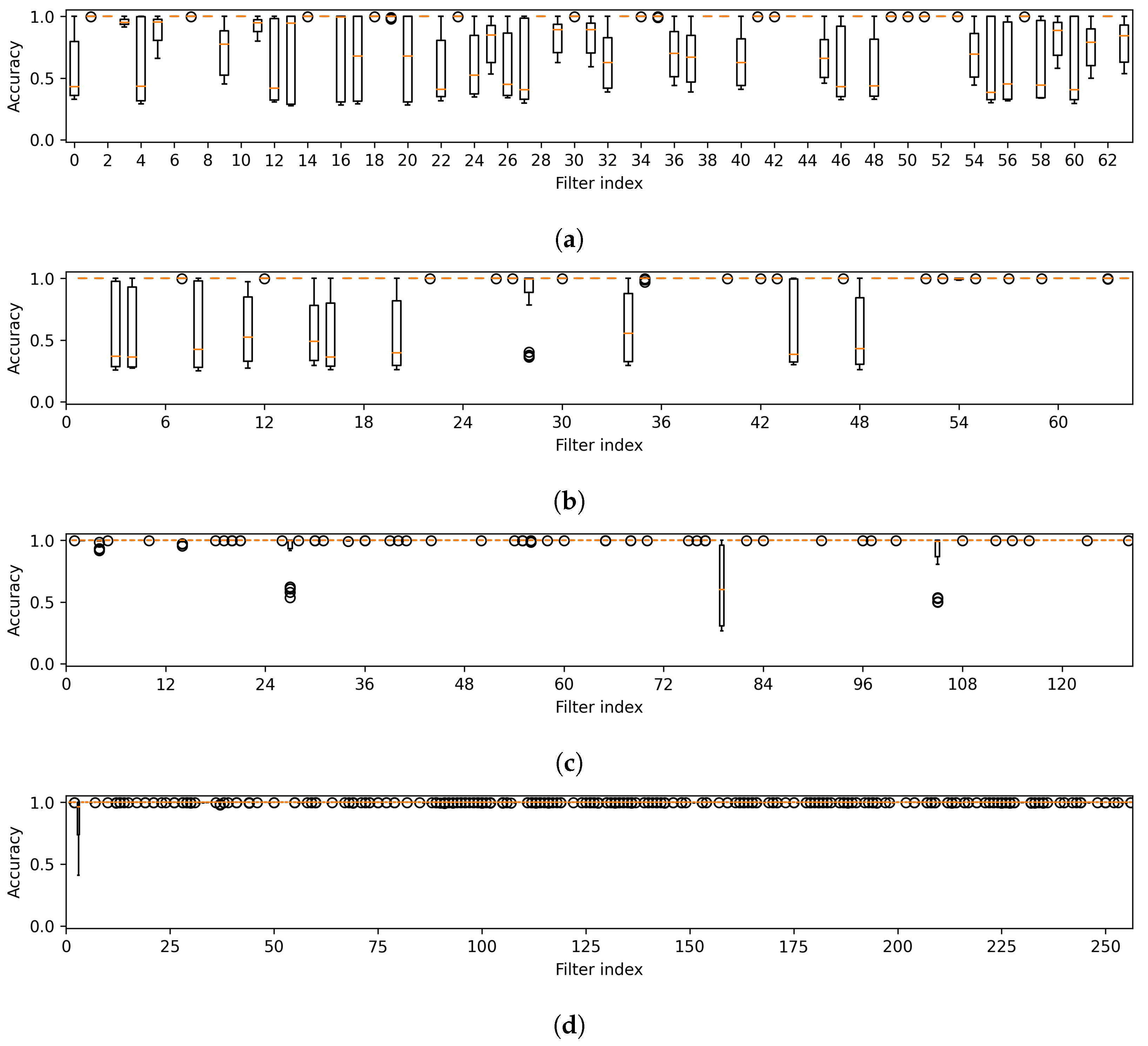
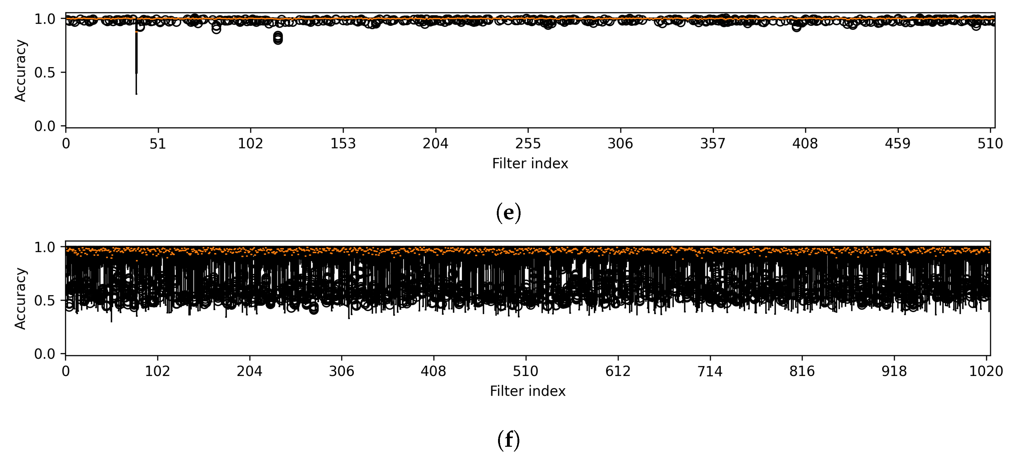
Figure 5.
Variability in accuracy across all attack methods is noted for features from the first layer (a), which is part of the first component, and from the intermediate layers (b–f), corresponding to the subsequent components of U-Net. Note that the results were obtained from a CT segmentation model.
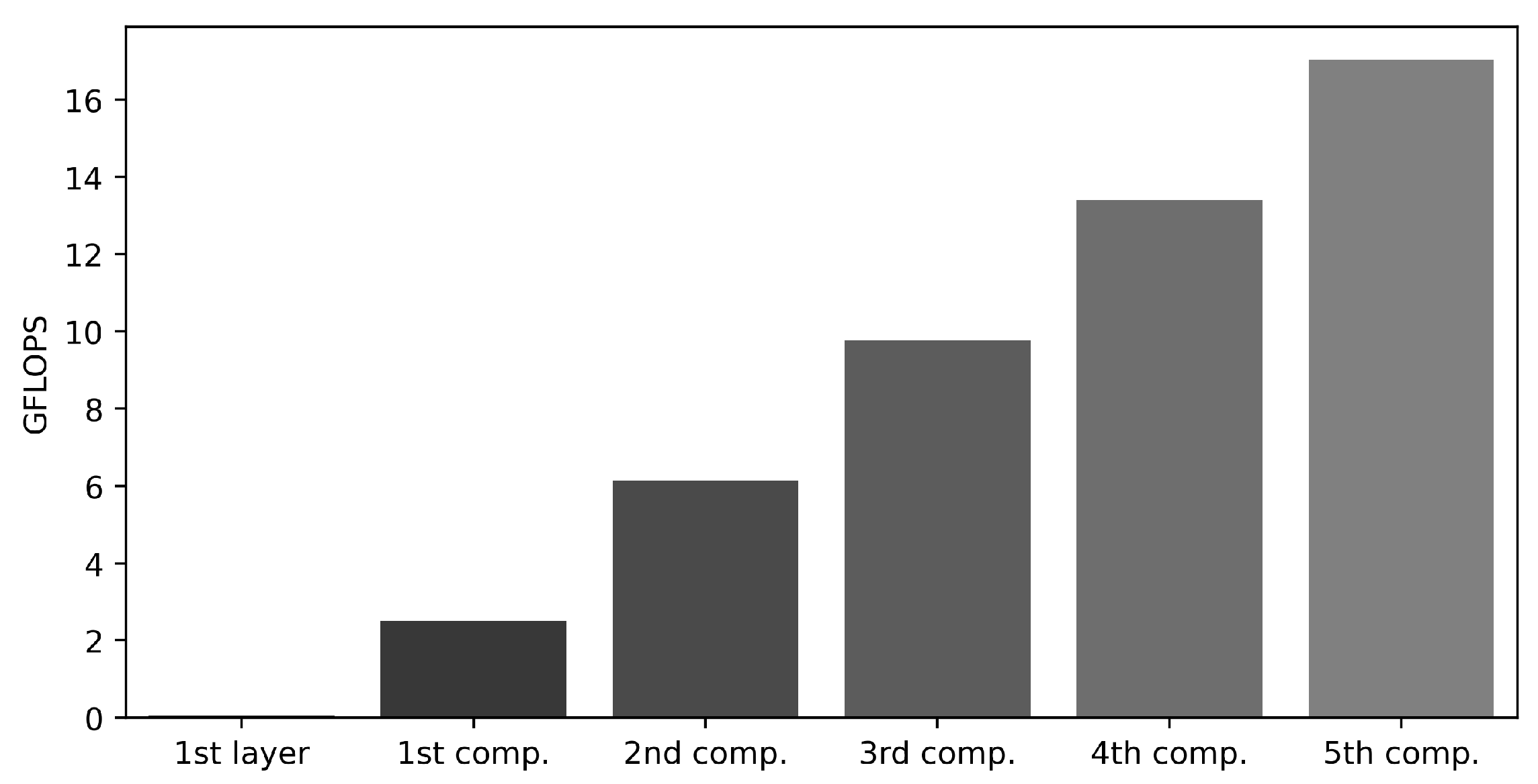
Figure 6.
GFLOPS comparison across components, illustrating the GFLOPS for the first layer within the first component and separately for each of the first to fifth components.
Figure 6.
GFLOPS comparison across components, illustrating the GFLOPS for the first layer within the first component and separately for each of the first to fifth components.
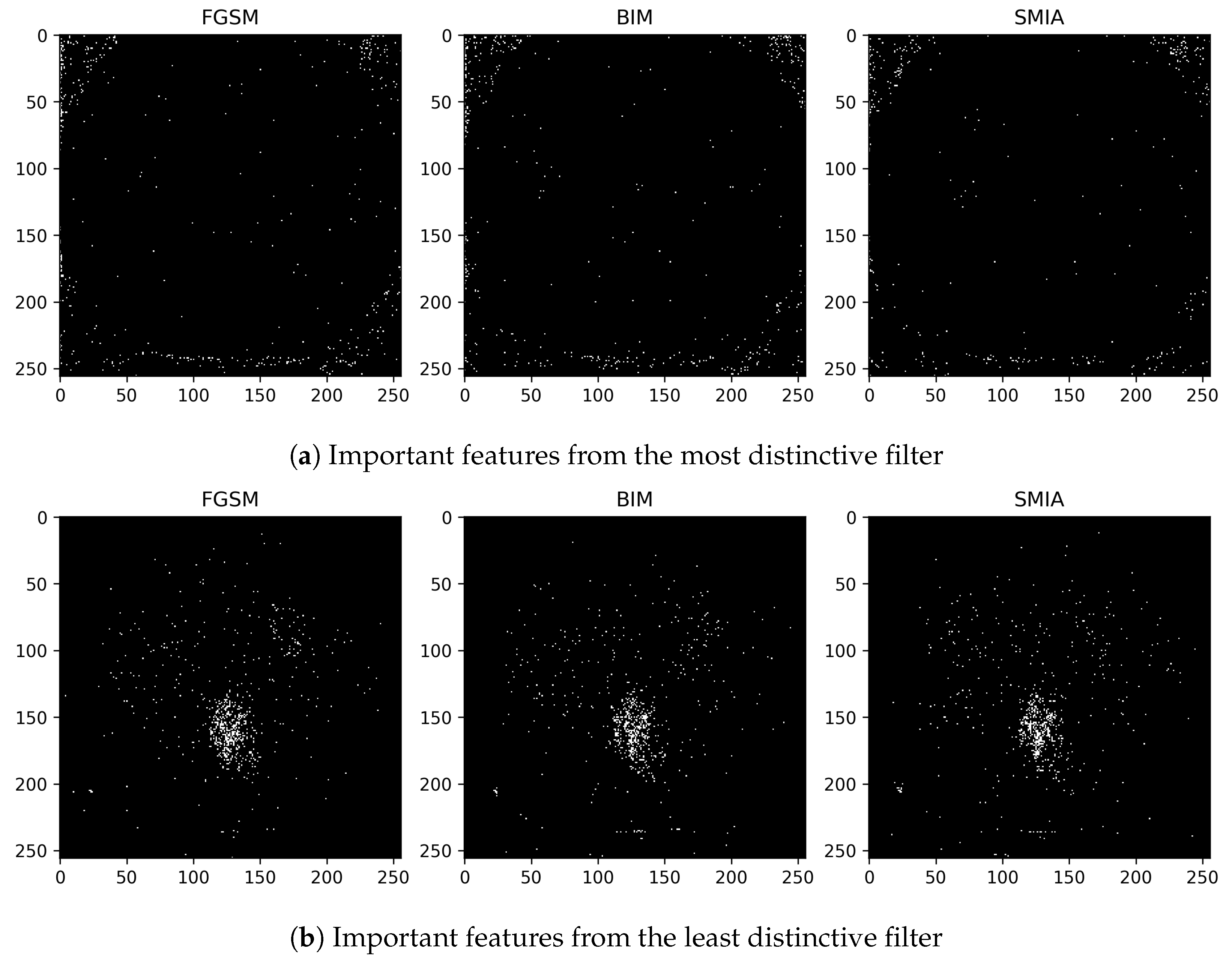
Figure 7.
Visualization of the top 1% of important features from classifiers trained using (a) the distinctive filter number 2 and (b) other than the distinctive filter number 22. These features are derived using the mean decrease in impurity from a random forest classifier for CT segmentation model.
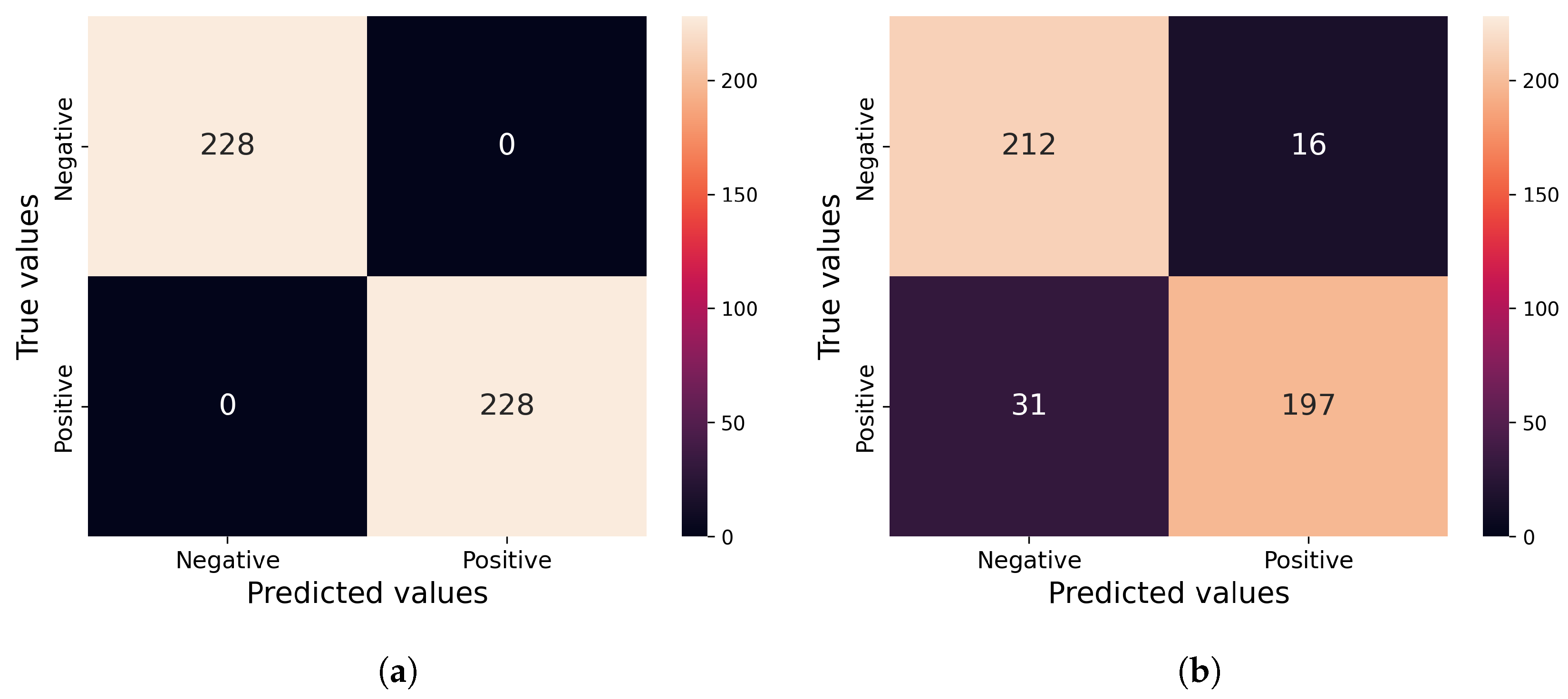
Figure 8.
(
a) Proposed method in this work; (
b) Baseline based on the previous work [
10]. Confusion matrices for (
a) our method and (
b) Park_spatial, which achieved the second-best performance on SMIA tests with an epsilon of 0.1 and 15 iterations for CT segmentation model.
Figure 8.
(
a) Proposed method in this work; (
b) Baseline based on the previous work [
10]. Confusion matrices for (
a) our method and (
b) Park_spatial, which achieved the second-best performance on SMIA tests with an epsilon of 0.1 and 15 iterations for CT segmentation model.
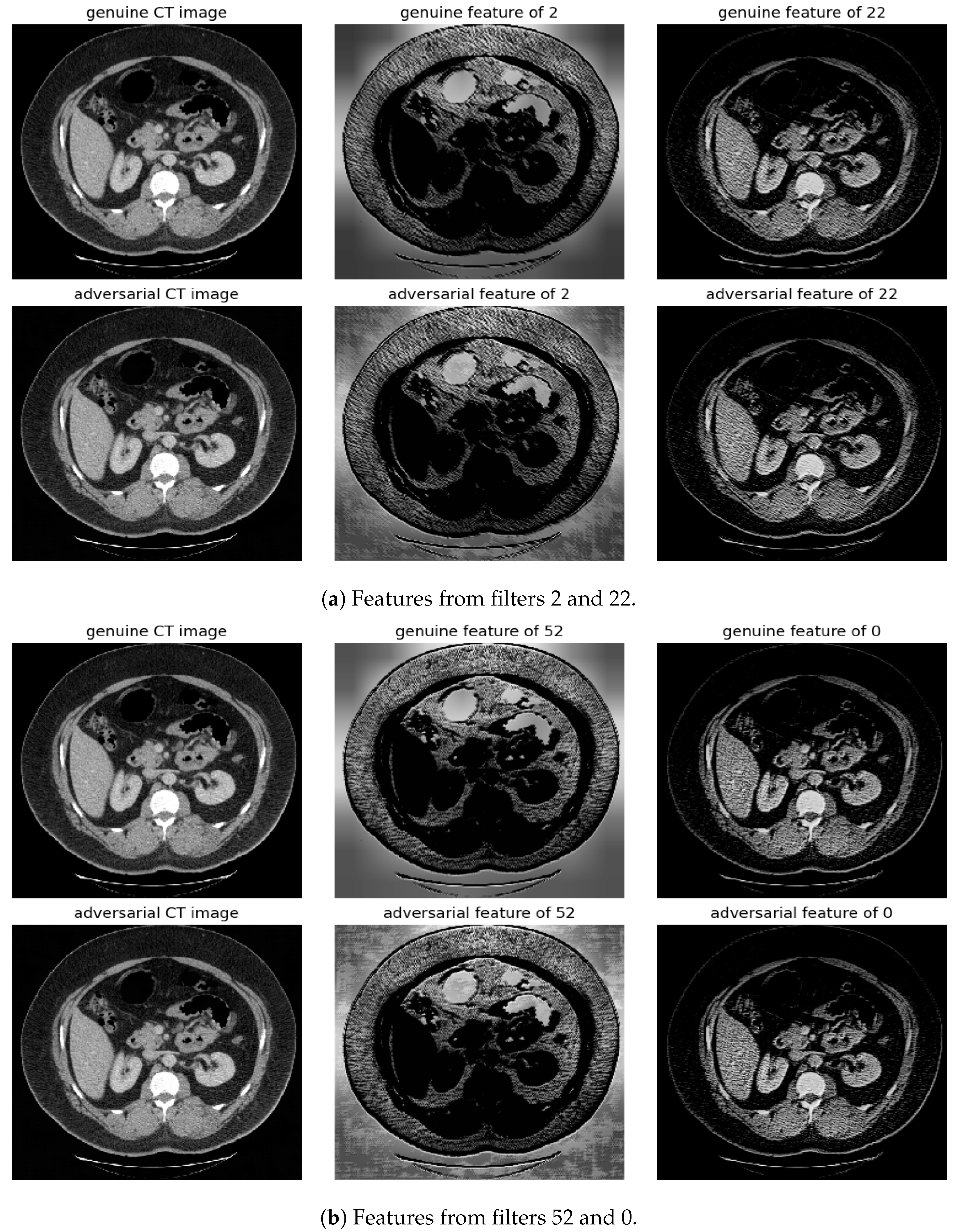
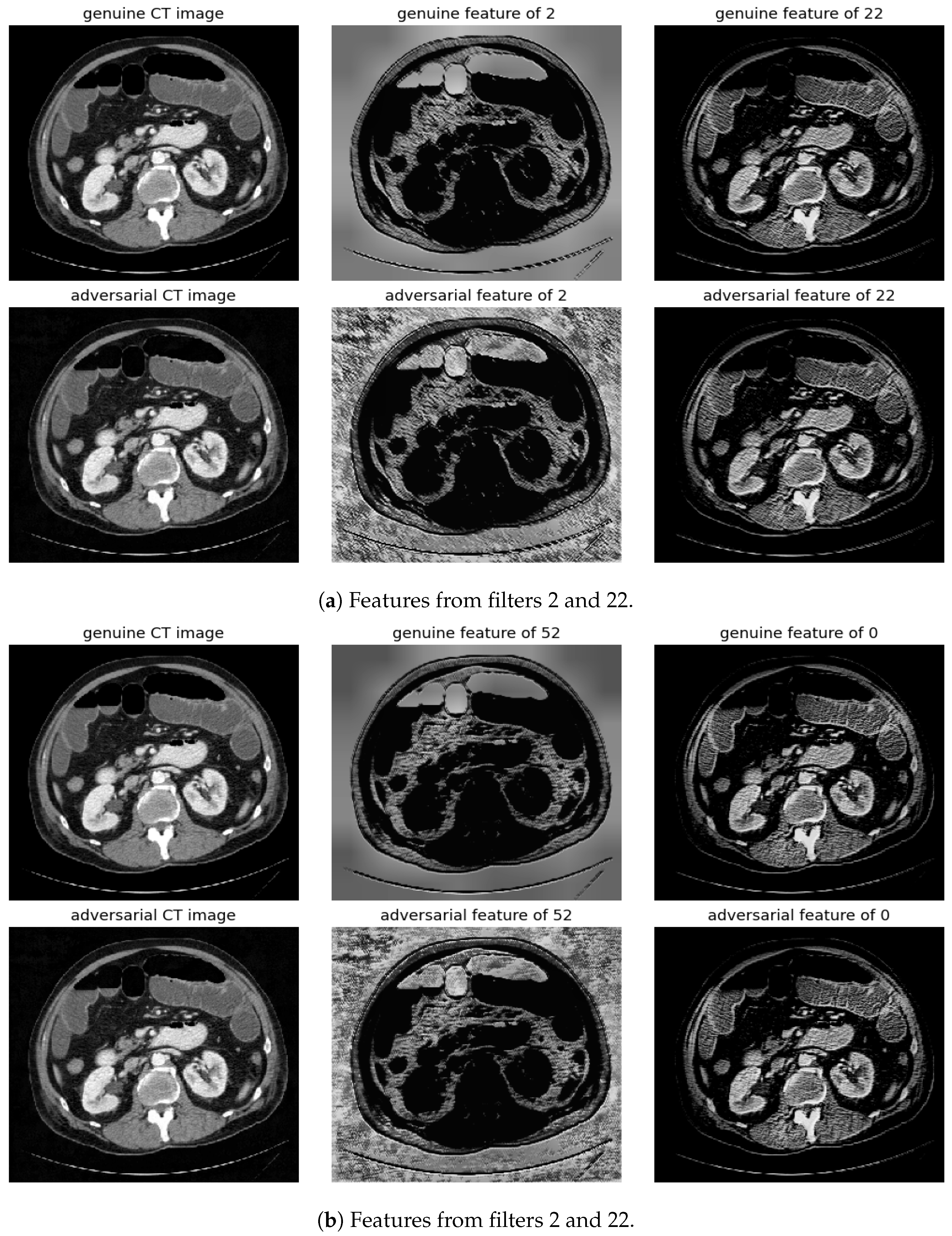
Figure 9.
Visualization under FGSM Attack: Comparison of features from the first layer between genuine and adversarial samples for the most sensitive (filters 2 and 52) and least sensitive (filters 22 and 0) filters.
Figure 9.
Visualization under FGSM Attack: Comparison of features from the first layer between genuine and adversarial samples for the most sensitive (filters 2 and 52) and least sensitive (filters 22 and 0) filters.
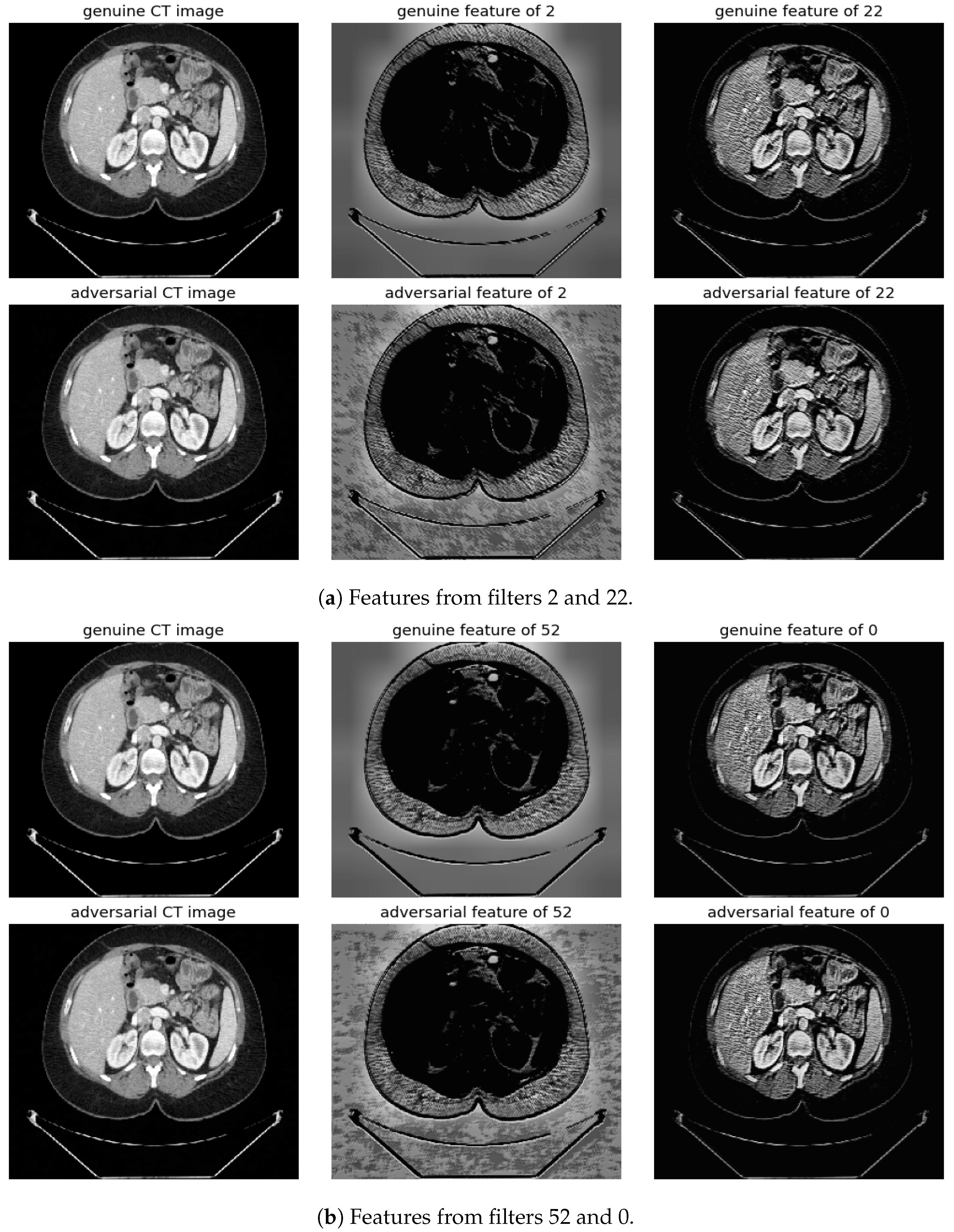
Figure 10.
Visualization under BIM Attack: Comparisons of features from the first layer between genuine and adversarial samples for the most sensitive (filters 2 and 52) and least sensitive (filters 22 and 0) filters.
Figure 10.
Visualization under BIM Attack: Comparisons of features from the first layer between genuine and adversarial samples for the most sensitive (filters 2 and 52) and least sensitive (filters 22 and 0) filters.
Figure 11.
Visualization under SMIA Attack: Comparison of features from the first layer between genuine and adversarial samples for the most sensitive (filters 2 and 52) and least sensitive (filter 22 and 0) filters.
Figure 11.
Visualization under SMIA Attack: Comparison of features from the first layer between genuine and adversarial samples for the most sensitive (filters 2 and 52) and least sensitive (filter 22 and 0) filters.
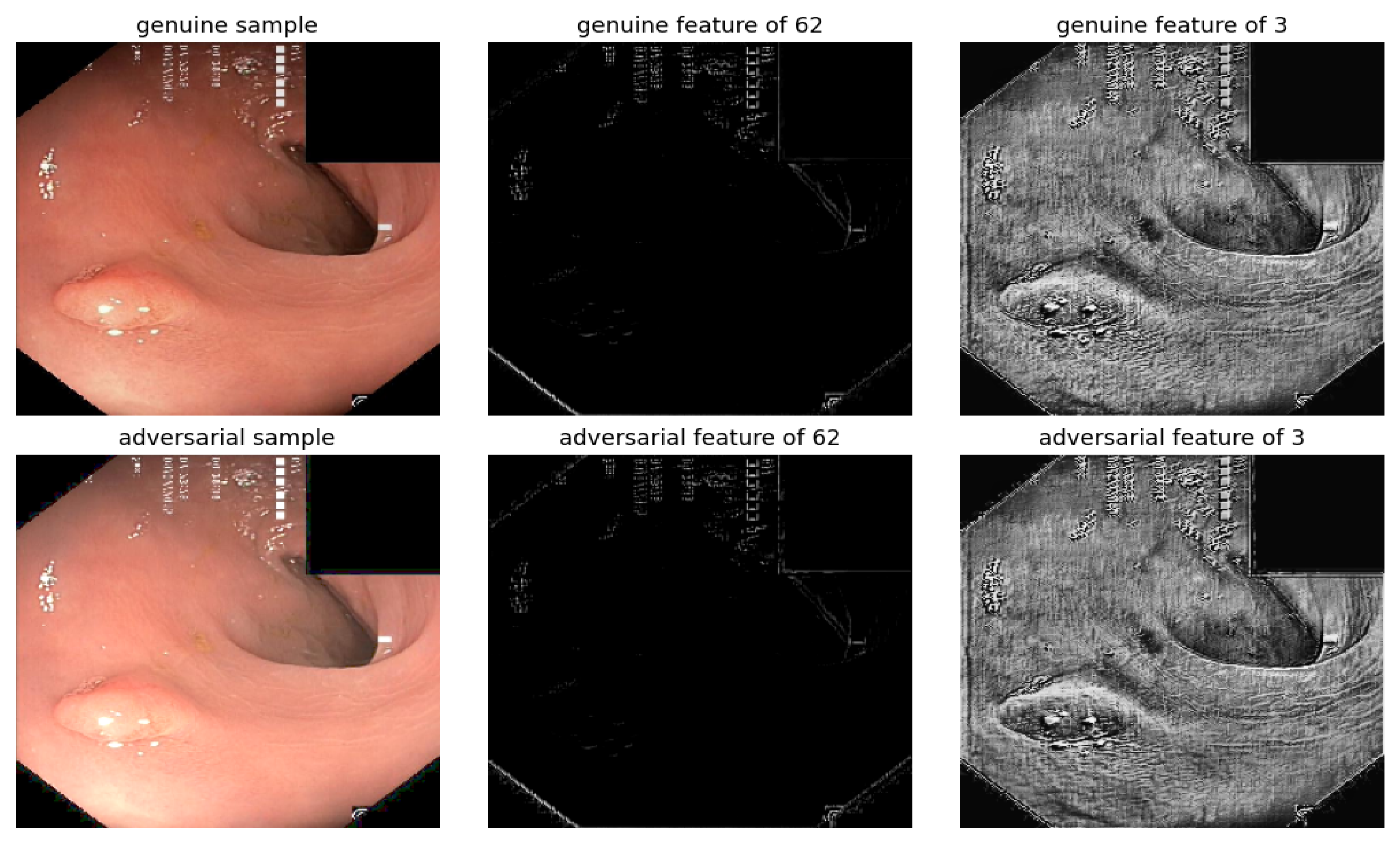
Figure 12.
Visualization under BIM attack, with EPS set to 0.01 and NITER at 15, of a gastrointestinal polyp image: Comparison of features from the first layer between genuine and adversarial samples for the most sensitive filters 62 and least sensitive filters 3.
Figure 12.
Visualization under BIM attack, with EPS set to 0.01 and NITER at 15, of a gastrointestinal polyp image: Comparison of features from the first layer between genuine and adversarial samples for the most sensitive filters 62 and least sensitive filters 3.
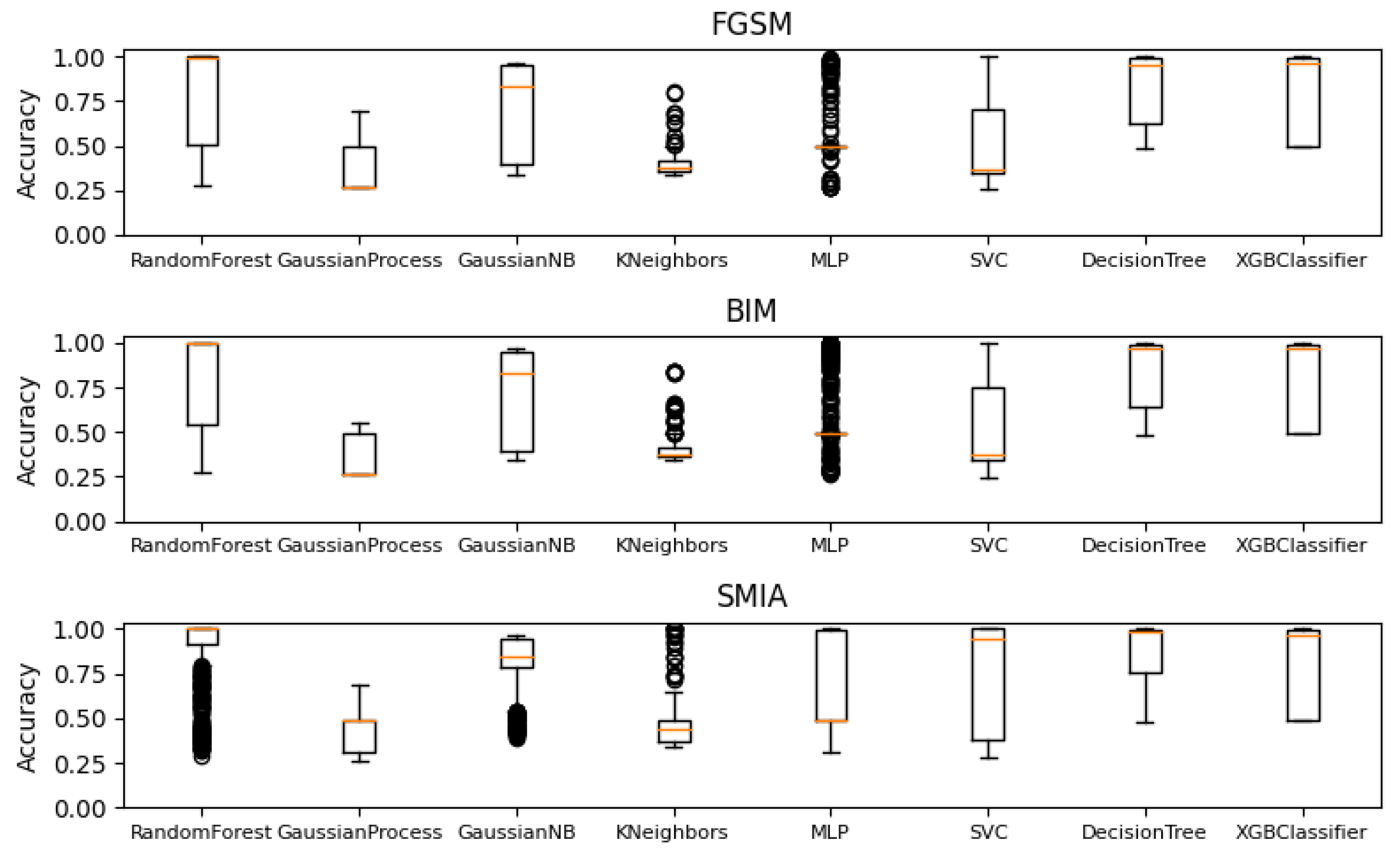
Figure 13.
Box plots illustrating the performance of various classifiers across different attack configurations, including parameters like the number of iterations and perturbation levels (EPS) for CT segmentation model.
Figure 13.
Box plots illustrating the performance of various classifiers across different attack configurations, including parameters like the number of iterations and perturbation levels (EPS) for CT segmentation model.
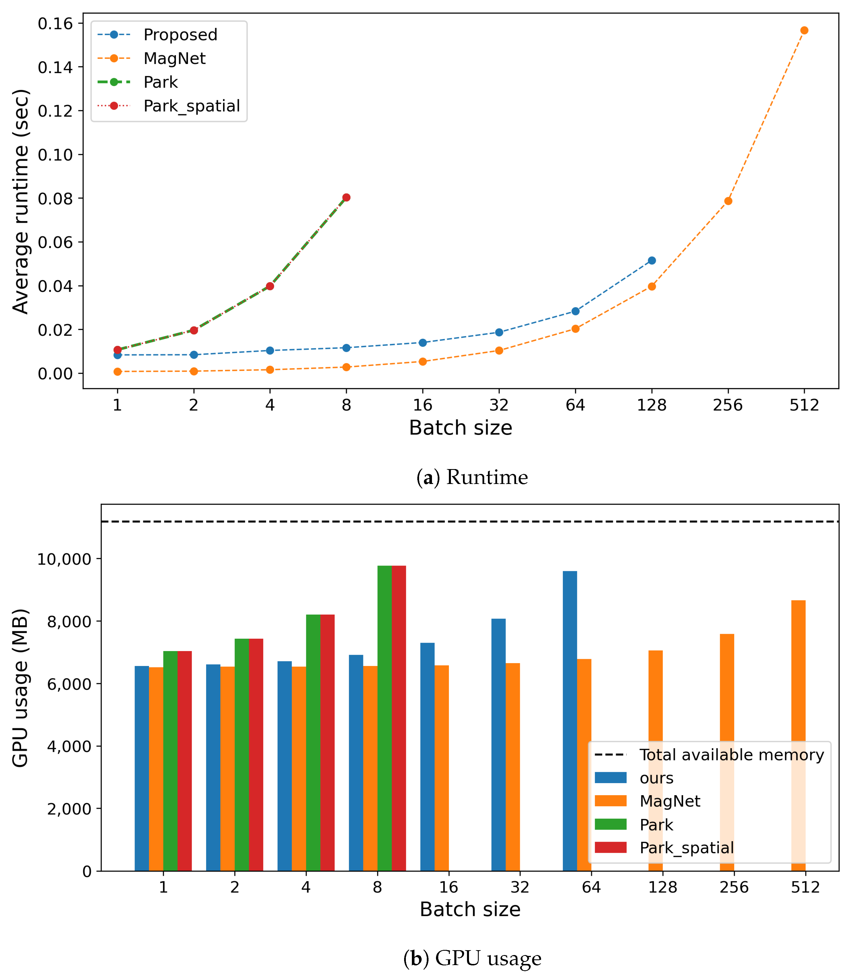
Figure 14.
Comparison of computation costs during inference, including (a) runtime and (b) GPU usage, across different methods.
Figure 14.
Comparison of computation costs during inference, including (a) runtime and (b) GPU usage, across different methods.
Table 1.
Summary of the target model architecture based on U-Net.
Table 1.
Summary of the target model architecture based on U-Net.
| Component | Operation | In Channels | Out Channels |
|---|
| Input | DoubleConv 1 | 1 or 3 | 64 |
| Down 1 | MaxPool 2 + DoubleConv | 64 | 128 |
| Down 2 | MaxPool + DoubleConv | 128 | 256 |
| Down 3 | MaxPool + DoubleConv | 256 | 512 |
| Down 4 | MaxPool + DoubleConv | 512 | 1024 |
| Up 3 1 | Upsample + DoubleConv | 1024 | 512 |
| Up 2 | Upsample + DoubleConv | 512 | 256 |
| Up 3 | Upsample + DoubleConv | 256 | 128 |
| Up 4 | Upsample + DoubleConv | 128 | 64 |
| Output | Conv2d | 64 | 14 or 2 |
Table 2.
Key features of methods.
Table 2.
Key features of methods.
| Method Name | Key Features |
|---|
| Ours | 1. Uses the target medical segmentation model |
| 2. Extracts features from the first layer |
| 3. Requires knowledge of the attack method to train the attack detector |
| MagNet | 1. Employs a shallow autoencoder |
| 2. Detects attacks based on the threshold of reconstruction error |
| 3. Does not require knowledge of the attack method |
| Park | 1. Utilizes the entire structure of the target medical segmentation model |
| 2. Transforms the given image using discrete Fourier transformation |
| 3. Does not require knowledge of the attack method |
| Park_spatial | 1. Utilizes the entire structure of the target medical segmentation model |
| 2. Does not transform the given image |
| 3. Does not require knowledge of the attack method |
Table 3.
Comparison of dice scores of CT segmentation for adversarial samples generated using FGSM, BIM, and SMIA, originating from a baseline dice score of 0.4524.
Table 3.
Comparison of dice scores of CT segmentation for adversarial samples generated using FGSM, BIM, and SMIA, originating from a baseline dice score of 0.4524.
| Attack | | EPS | 0.01 | 0.02 | 0.1 |
|---|
| NITR | |
|---|
| FGSM | | | 0.4164 | 0.3924 | 0.2555 |
| BIM | 5 | 0.4195 | 0.3845 | 0.2254 |
| 10 | 0.4260 | 0.3910 | 0.2330 |
| 15 | 0.4263 | 0.3900 | 0.2254 |
| SMIA | 5 | 0.3967 | 0.3518 | 0.1707 |
| 10 | 0.3681 | 0.2967 | 0.1168 |
| 15 | 0.3322 | 0.2492 | 0.0907 |
Table 4.
Comparison of dice scores of gastrointestinal polyp dataset for adversarial samples generated using FGSM, BIM, and SMIA, originating from a baseline dice score of 0.8886.
Table 4.
Comparison of dice scores of gastrointestinal polyp dataset for adversarial samples generated using FGSM, BIM, and SMIA, originating from a baseline dice score of 0.8886.
| Attack | | EPS | 0.01 | 0.1 | 0.5 |
|---|
| NITR | |
|---|
| FGSM | | | 0.8886 | 0.8813 | 0.6950 |
| BIM | 5 | 0.8872 | 0.6950 | 0.4591 |
| 10 | 0.8813 | 0.4591 | 0.4591 |
| 15 | 0.8713 | 0.4591 | 0.4591 |
| SMIA | 5 | 0.8872 | 0.6950 | 0.4591 |
| 10 | 0.8813 | 0.4591 | 0.4591 |
| 15 | 0.8712 | 0.4591 | 0.4591 |
Table 5.
Classification accuracy of adversarial sample detection using selected filters by proposed framework in this work for CT segmentation model.
Table 5.
Classification accuracy of adversarial sample detection using selected filters by proposed framework in this work for CT segmentation model.
| Attack | Filter | | EPS | 0.01 | 0.02 | 0.1 |
|---|
| NITR | |
|---|
| FGSM | 22 | | | 0.6820 | 0.6623 | 0.8531 |
| 2 | | | 1.0000 | 1.0000 | 1.0000 |
| BIM | 22 | 5 | 0.6732 | 0.6732 | 0.8838 |
| 10 | 0.6557 | 0.6294 | 0.8640 |
| 15 | 0.6623 | 0.6535 | 0.8596 |
| 2 | 5 | 1.0000 | 1.0000 | 1.0000 |
| 10 | 1.0000 | 1.0000 | 1.0000 |
| 15 | 1.0000 | 1.0000 | 1.0000 |
| SMIA | 22 | 5 | 0.6557 | 0.7149 | 1.0000 |
| 10 | 0.6842 | 0.7346 | 1.0000 |
| 15 | 0.6886 | 0.8136 | 1.0000 |
| 2 | 5 | 1.0000 | 1.0000 | 1.0000 |
| 10 | 1.0000 | 1.0000 | 1.0000 |
| 15 | 1.0000 | 1.0000 | 1.0000 |
Table 6.
Comparative analysis of adversarial sample against CT imaging dataset detection accuracy across various methods. Note that the proposed approach in this work exclusively utilizes features from filter number 2.
Table 6.
Comparative analysis of adversarial sample against CT imaging dataset detection accuracy across various methods. Note that the proposed approach in this work exclusively utilizes features from filter number 2.
| Attack | Method | | EPS | 0.01 | 0.1 | 0.5 |
|---|
| NITR | |
|---|
| FGSM | Ours | | | 1.0000 | 1.0000 | 1.0000 |
| MagNet | | | 0.4956 | 0.4934 | 0.4890 |
| Park | | | 0.4956 | 0.4956 | 0.4890 |
| Park_spatial | | | 0.4956 | 0.4912 | 0.4759 |
| BIM | Ours | 5 | 1.0000 | 1.0000 | 1.0000 |
| 10 | 1.0000 | 1.0000 | 1.0000 |
| 15 | 1.0000 | 1.0000 | 1.0000 |
| MagNet | 5 | 0.4956 | 0.4934 | 0.4890 |
| 10 | 0.4956 | 0.4934 | 0.4890 |
| 15 | 0.4956 | 0.4956 | 0.4890 |
| Park | 5 | 0.4956 | 0.4934 | 0.4846 |
| 10 | 0.4956 | 0.4934 | 0.4868 |
| 15 | 0.4956 | 0.4934 | 0.4868 |
| Park_spatial | 5 | 0.4934 | 0.4825 | 0.4693 |
| 10 | 0.4934 | 0.4825 | 0.4693 |
| 15 | 0.4934 | 0.4846 | 0.4671 |
| SMIA | Ours | 5 | 1.0000 | 1.0000 | 1.0000 |
| 10 | 1.0000 | 1.0000 | 1.0000 |
| 15 | 1.0000 | 1.0000 | 1.0000 |
| MagNet | 5 | 0.4934 | 0.4890 | 0.4890 |
| 10 | 0.4912 | 0.4890 | 0.4890 |
| 15 | 0.4890 | 0.4890 | 0.4890 |
| Park | 5 | 0.4934 | 0.4846 | 0.5000 |
| 10 | 0.4890 | 0.4846 | 0.5482 |
| 15 | 0.4890 | 0.4846 | 0.8223 |
| Park_spatial | 5 | 0.4846 | 0.4693 | 0.4956 |
| 10 | 0.4737 | 0.4649 | 0.5943 |
| 15 | 0.4715 | 0.4649 | 0.8969 |
Table 7.
Comparative analysis of PPV and sensitivity in adversarial attack detection across different methods and types of attacks using CT imaging dataset.
Table 7.
Comparative analysis of PPV and sensitivity in adversarial attack detection across different methods and types of attacks using CT imaging dataset.
| Attack | Method | | EPS | 0.01 | 0.02 | 0.1 |
|---|
| NITR | | PPV | Sensitivity | PPV | Sensitivity | PPV | Sensitivity |
|---|
| FGSM | ours | | | 1.0000 | 1.0000 | 1.0000 | 1.0000 | 1.0000 | 1.0000 |
| MagNet | | | 0.3750 | 0.0132 | 0.2857 | 0.0088 | 0.0000 | 0.0000 |
| Park | | | 0.4167 | 0.0219 | 0.4167 | 0.0219 | 0.2222 | 0.0088 |
| Park_spatial | | | 0.4667 | 0.0614 | 0.4286 | 0.0526 | 0.2381 | 0.0219 |
| BIM | Ours | 5 | 1.0000 | 1.0000 | 1.0000 | 1.0000 | 1.0000 | 1.0000 |
| 10 | 1.0000 | 1.0000 | 1.0000 | 1.0000 | 1.0000 | 1.0000 |
| 15 | 1.0000 | 1.0000 | 1.0000 | 1.0000 | 1.0000 | 1.0000 |
| MagNet | 5 | 0.3750 | 0.0132 | 0.2857 | 0.0088 | 0.0000 | 0.0000 |
| 10 | 0.3750 | 0.0132 | 0.2857 | 0.0088 | 0.0000 | 0.0000 |
| 15 | 0.3750 | 0.0132 | 0.3750 | 0.0132 | 0.0000 | 0.0000 |
| Park | 5 | 0.4167 | 0.0219 | 0.3636 | 0.0175 | 0.0000 | 0.0000 |
| 10 | 0.4167 | 0.0219 | 0.3636 | 0.0175 | 0.1250 | 0.0044 |
| 15 | 0.4167 | 0.0219 | 0.3636 | 0.0175 | 0.1250 | 0.0044 |
| Park_spatial | 5 | 0.4483 | 0.0570 | 0.3333 | 0.0351 | 0.1111 | 0.0088 |
| 10 | 0.4483 | 0.0570 | 0.3333 | 0.0351 | 0.1111 | 0.0088 |
| 15 | 0.4483 | 0.0570 | 0.3600 | 0.0395 | 0.0588 | 0.0044 |
| SMIA | Ours | 5 | 1.0000 | 1.0000 | 1.0000 | 1.0000 | 1.0000 | 1.0000 |
| 10 | 1.0000 | 1.0000 | 1.0000 | 1.0000 | 1.0000 | 1.0000 |
| 15 | 1.0000 | 1.0000 | 1.0000 | 1.0000 | 1.0000 | 1.0000 |
| MagNet | 5 | 0.2857 | 0.0088 | 0.0000 | 0.0000 | 0.0000 | 0.0000 |
| 10 | 0.1667 | 0.0044 | 0.0000 | 0.0000 | 0.0000 | 0.0000 |
| 15 | 0.0000 | 0.0000 | 0.0000 | 0.0000 | 0.0000 | 0.0000 |
| Park | 5 | 0.3636 | 0.0175 | 0.0000 | 0.0000 | 0.5000 | 0.0307 |
| 10 | 0.2222 | 0.0088 | 0.0000 | 0.0000 | 0.8056 | 0.1272 |
| 15 | 0.2222 | 0.0088 | 0.0000 | 0.0000 | 0.9565 | 0.6754 |
| Park_spatial | 5 | 0.3600 | 0.0395 | 0.1111 | 0.0088 | 0.4667 | 0.0614 |
| 10 | 0.2000 | 0.0175 | 0.0000 | 0.0000 | 0.7867 | 0.2588 |
| 15 | 0.1579 | 0.0132 | 0.0000 | 0.0000 | 0.9249 | 0.8640 |
Table 8.
Comparative analysis of PPV and sensitivity in adversarial attack detection across different methods and types of attacks using gastrointestinal polyp dataset.
Table 8.
Comparative analysis of PPV and sensitivity in adversarial attack detection across different methods and types of attacks using gastrointestinal polyp dataset.
| Attack | Method | | EPS | 0.01 | 0.1 | 0.5 |
|---|
| NITR | | PPV | Sensitivity | PPV | Sensitivity | PPV | Sensitivity |
|---|
| FGSM | Ours | | | 0.9383 | 0.9120 | 0.9881 | 1.0000 | 1.0000 | 1.0000 |
| MagNet | | | NaN | 0.0000 | NaN | 0.0000 | 1.0000 | 0.0520 |
| Park | | | NaN | 0.0000 | NaN | 0.0000 | 1.0000 | 0.0640 |
| Park_spatial | | | NaN | 0.0000 | NaN | 0.0000 | 1.0000 | 0.0280 |
| BIM | Ours | 5 | 1.0000 | 1.0000 | 1.0000 | 1.0000 | 1.0000 | 1.0000 |
| 10 | 1.0000 | 1.0000 | 1.0000 | 1.0000 | 1.0000 | 1.0000 |
| 15 | 1.0000 | 1.0000 | 1.0000 | 1.0000 | 1.0000 | 1.0000 |
| MagNet | 5 | 1.0000 | 0.0520 | 1.0000 | 0.2840 | NaN | 0.0000 |
| 10 | NaN | 0.0000 | 1.0000 | 0.2840 | 1.0000 | 0.2840 |
| 15 | NaN | 0.0000 | 1.0000 | 0.2840 | 1.0000 | 0.2840 |
| Park | 5 | NaN | 0.0000 | 1.0000 | 0.0640 | 1.0000 | 0.5680 |
| 10 | NaN | 0.0000 | 1.0000 | 0.5680 | 1.0000 | 0.5680 |
| 15 | NaN | 0.0000 | 1.0000 | 0.5680 | 1.0000 | 0.5680 |
| Park_spatial | 5 | NaN | 0.0000 | 1.0000 | 0.0280 | 1.0000 | 0.0880 |
| 10 | NaN | 0.0000 | 1.0000 | 0.0880 | 1.0000 | 0.0880 |
| 15 | NaN | 0.0000 | 1.0000 | 0.0880 | 1.0000 | 0.0880 |
| SMIA | Ours | 5 | 1.0000 | 1.0000 | 1.0000 | 1.0000 | 1.0000 | 1.0000 |
| 10 | 1.0000 | 1.0000 | 1.0000 | 1.0000 | 1.0000 | 1.0000 |
| 15 | 1.0000 | 1.0000 | 1.0000 | 1.0000 | 1.0000 | 1.0000 |
| MagNet | 5 | NaN | 0.0000 | 1.0000 | 0.0520 | 1.0000 | 0.2840 |
| 10 | NaN | 0.0000 | 1.0000 | 0.2840 | 1.0000 | 0.2840 |
| 15 | NaN | 0.0000 | 1.0000 | 0.2840 | 1.0000 | 0.2840 |
| Park | 5 | NaN | 0.0000 | 1.0000 | 0.0640 | 1.0000 | 0.5680 |
| 10 | NaN | 0.0000 | 1.0000 | 0.5680 | 1.0000 | 0.5680 |
| 15 | NaN | 0.0000 | 1.0000 | 0.5680 | 1.0000 | 0.5680 |
| Park_spatial | 5 | NaN | 0.0000 | 1.0000 | 0.0280 | 1.0000 | 0.0880 |
| 10 | NaN | 0.0000 | 1.0000 | 0.0880 | 1.0000 | 0.0880 |
| 15 | NaN | 0.0000 | 1.0000 | 0.0880 | 1.0000 | 0.0880 |


