Article

The Spatiotemporal Variation in Biodiversity and Its Response to Different Future Development Scenarios: A Case Study of Guilin as an Internationally Renowned Tourist Destination in China

1
College of Geomatics and Geoinformation, Guilin University of Technology, Guilin 541004, China
2
Guangxi Key Laboratory of Spatial Information and Geomatics, Guilin University of Technology, Guilin 541004, China
*
Author to whom correspondence should be addressed.
Appl. Sci. 2024, 14(5), 2101; https://doi.org/10.3390/app14052101
Submission received: 31 January 2024 / Revised: 29 February 2024 / Accepted: 1 March 2024 / Published: 2 March 2024

Abstract

:
The preservation of biodiversity is crucial for maintaining ecological balance and promoting the harmonious development of mankind and nature. To formulate a biodiversity conservation plan for Guilin in China and accurately evaluate the impact of conservation measures on regional biodiversity, this study combined the InVEST model (v 3.7.0), the GeoSOS-FLUS model (v 2.3), and the landscape pattern index, analyzing the spatiotemporal changes in biodiversity from 2000 to 2020 in Guilin and simulating biodiversity under different development scenarios in 2040. The results showed the following: (1) The biodiversity index in Guilin displayed a declining trend, with the average annual value decreasing from 0.875 in 2000 to 0.870 in 2020. The area experiencing a reduction in biodiversity was primarily concentrated around the city. (2) The biodiversity level of each district and county had a large spatiotemporal difference, with the overall distribution characteristics of “higher in the northwest, southwest, and east, and lower in the northeast, southeast and central”. (3) The biodiversity hotspots were identified as priority areas for conservation; woodland and wetland were effectively protected, and the expansion of construction land and arable land was limited under the ecological protection scenario compared with the natural development scenario. (4) The annual average value of the biodiversity index of Guilin could reach 0.872 in 2040 after the adoption of ecological conservation measures, which is 0.013 higher than the natural development scenario. The results of this study can provide guidance for the construction of a national sustainable development model city and land use planning in Guilin, as well as a scientific reference for the creation of biodiversity conservation policies.

1. Introduction

Biodiversity is an umbrella term for all living organisms and the environment in which they live, serving as the foundational basis and essential guarantee for human survival and development [1,2]. Despite the increasing efforts in global biodiversity conservation in recent decades, the world continues to face significant challenges due to ongoing biodiversity loss. This is exacerbated by factors such as global climate change [3], environmental pollution [4], invasive species [5], and the intensification of human activities [6]. Consequently, the quantitative assessment of regional biodiversity status and the formulation of rational and effective conservation measures have become central concerns for both governments and scholars.
The proxy indicator assessment method is a commonly used method to measure the status of regional biodiversity, which quantifies and visualizes the results of biodiversity assessments using data such as remotely sensed imagery [7]. Currently, scholars have conducted extensive studies employing the proxy indicator assessment method to investigate the spatiotemporal changes and influencing mechanisms of biodiversity across various scales [8,9,10,11]. However, the studies that have been carried out have focused on analyzing the current status of biodiversity, and few scholars have formulated site-specific measures for biodiversity conservation and testing in response to study findings. Land use/cover (LUC) change has long been widely recognized by the academic community as a major influence on biodiversity change [12,13]. Various intensities and types of LUC development activities exert influence on LUC and spatial patterns, consequently impacting ecological processes and biological behavior [14,15]. Therefore, employing LUC data alongside pertinent spatial analysis techniques allows for the effective identification of areas where biodiversity faces threats, thereby facilitating improved conservation planning strategies [16]. Moreover, the GeoSOS-FLUS model can simulate LUC patterns under diverse future scenarios and has found extensive application in studies related to the multi-scenario simulation of future LUC [17,18,19]. This model is often employed to simulate the LUC pattern under future natural development scenarios (NDSs) and ecological protection scenarios (EPSs). The efficacy of conservation measures can be assessed by comparing the impact of LUC changes on regional biodiversity across various scenarios.
The habitat quality index (HQI) is frequently utilized as a proxy indicator of biodiversity. It denotes the capacity of a habitat to furnish a stable living environment for organisms on a sustained basis and finds extensive application in biodiversity research [20,21]. It can reflect the biodiversity status of the region to some extent, and the assessment of changes in habitat quality (HQ) can provide a reference for regional LUC management and ecological conservation planning [22,23]. However, some research has demonstrated that the utilization of the HQI to evaluate biodiversity oversimplifies the physical mechanisms of ecosystems, leading to certain constraints in its assessment outcomes [24,25]. Few scholars have supplemented and improved this alternative index. Landscape structure is a concrete manifestation of landscape heterogeneity, reflecting the characteristics of landscape structure composition and spatial configuration. Its change alters material transport and information exchange within the landscape, thereby affecting various ecological processes [26]. Therefore, amalgamating a landscape structure index with an HQI to construct a composite biodiversity index has the accuracy to yield a more precise and comprehensive assessment of biodiversity.
Guilin is renowned for its distinctive karst landscape, showcasing a diverse array of flora and fauna that includes numerous rare organisms and endemic species, resulting in a high biodiversity conservation value [27]. Nevertheless, as urbanization has progressed in recent years, the natural land in Guilin has steadily shrunk, posing a significant threat to biodiversity. In this study, Guilin was selected as the research area, where the landscape pattern index and HQI were integrated to establish a comprehensive biodiversity index. The objectives of the study were to (1) quantitatively assess the spatiotemporal biodiversity changes in Guilin from 2000 to 2020; (2) identify biodiversity hotspots to reveal the spatiotemporal heterogeneity of biodiversity across different LUC types; and (3) simulate biodiversity in Guilin under different development scenarios for 2040 to validate the effectiveness of ecological conservation measures. The study results can provide scientific references for promoting the sustainable development of biodiversity in Guilin and enhancing biodiversity conservation efforts.

2. Study Area and Data Sources
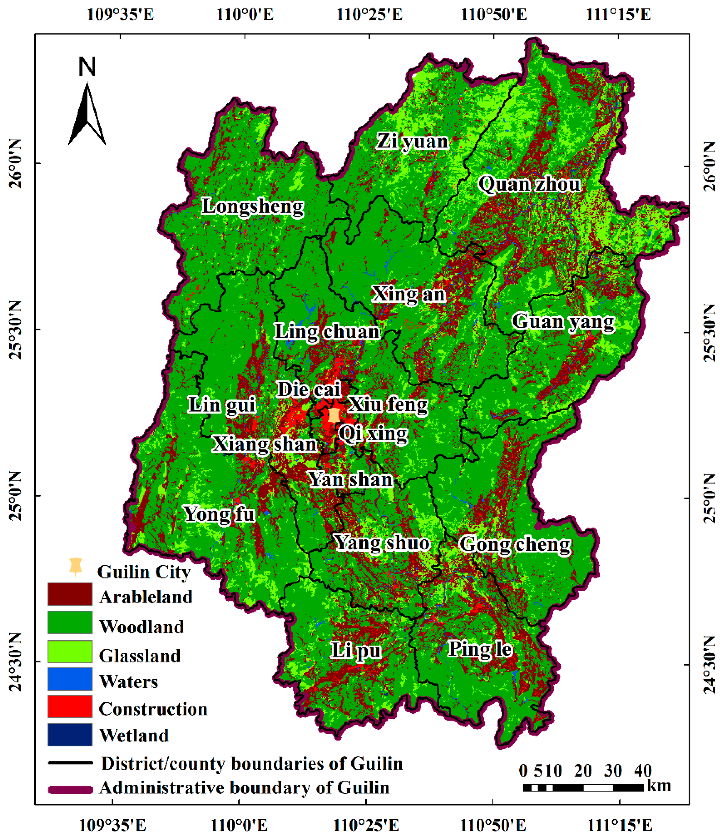
2.1. Study Area

Guilin is situated in the southwestern part of the Nanling mountain range and the northeastern region of the Guangxi Zhuang Autonomous Region in China (109°36′~111°29′ E, 24°15′~26°23′ N). The entire administrative area of Guilin spans 27,800 square kilometers, encompassing six urban districts and eleven counties (Figure 1). The elevated topography of Guilin in the west, north, and southeast, along with lower topography in the central part, is characterized predominantly by mid to low-mountainous terrain. It falls under the subtropical monsoon climate category and maintains an average annual temperature of 18.9 °C. The average annual rainfall is 1949.5 mm, with mild winters, hot summers, and a long rainy season [28]. There are many kinds of wild animals and plants in the city, including 545 kinds of terrestrial vertebrate wild animals, among which 69 kinds of rare and endangered animals are under national key protection. There are more than 1000 kinds of higher plants, including precious tree species such as silver fir and ginkgo biloba, and the resource fir is categorized as a critically endangered species on the IUCN Global Red List [5,29]. In addition, Guilin is abundant in ecological resources, characterized by complex and diverse landscape types. It hosts numerous nature reserves, forest parks, and wetland parks, including Huaping, Maoer Mountain, Qianjiadong, and Ziyuan County fir, comprising four national nature reserves [30].

2.2. Data Sources and Preprocessing
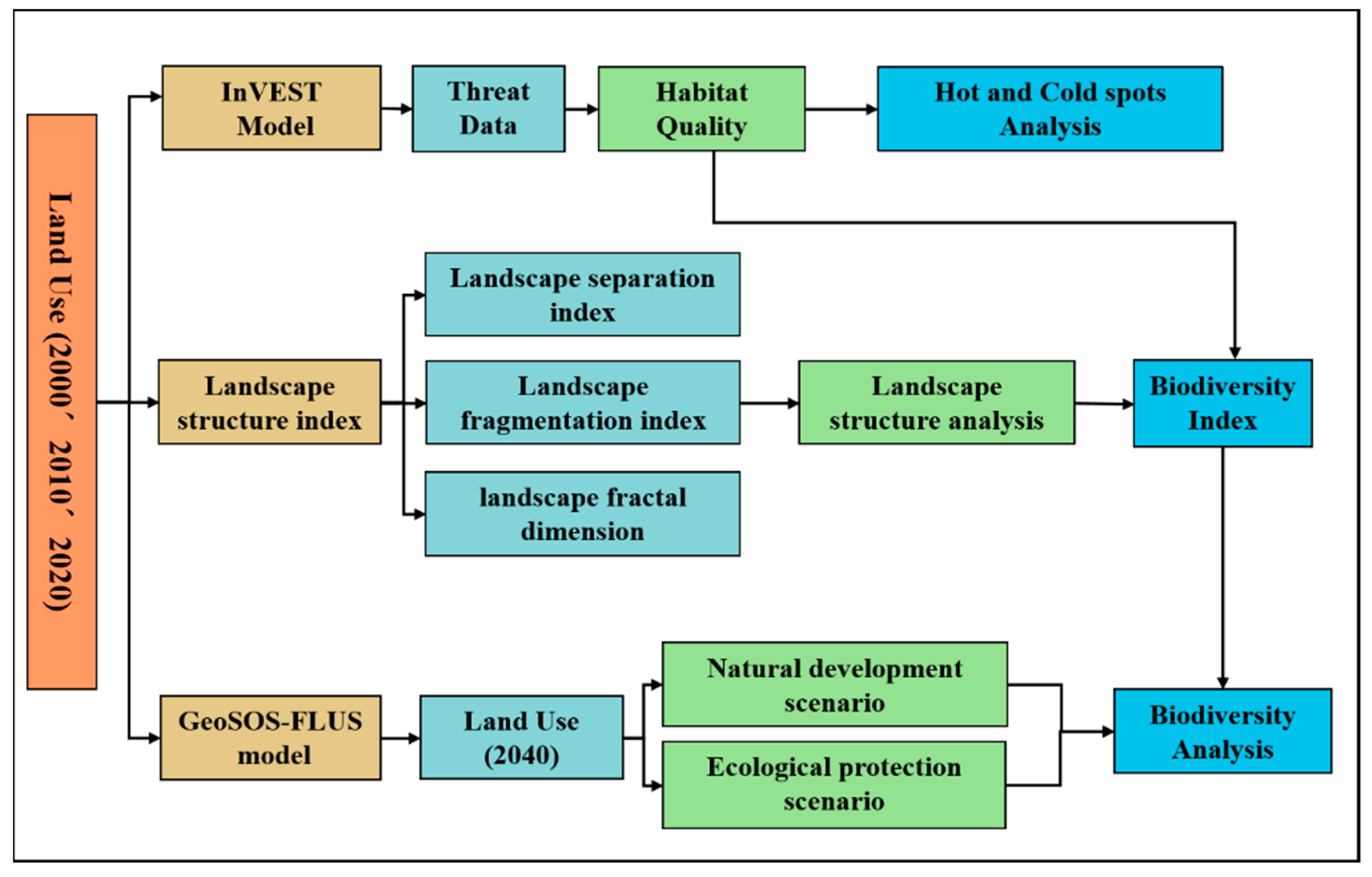
The LUC data of Guilin were obtained from the global land cover data of the National Basic Geographic Information Center (https://www.ngcc.cn/ (accessed on 16 June 2023)) in 2000, 2010, and 2020. The LUC types were mainly divided into the following six categories: arable land (AL), woodland (WL), grassland (GL), waters (WT), construction land (CL), and wetland (WTL), and the spatial resolution of the data was 30 m (Figure 1). The traffic data came from the National Basic Geographic Information Database, and, given the availability of the data, 1:100,000 road data were used for 2017. The digital elevation model (DEM) was obtained from the geospatial data platform (https://www.gscloud.cn/ (accessed on 28 June 2023)) with a spatial resolution of 30 m. Slope and aspect data were derived from it using ArcGIS software (v 10.6). Annual rainfall, average annual temperature, and GDP data were obtained from the Resources and Environmental Sciences and Data Center of the Chinese Academy of Sciences (https://www.resdc.cn/ (accessed on 3 July 2023)), with a spatial resolution of 1 km.

2.3. Methods

The research framework of this study is shown in Figure 2. Firstly, LUC data were employed to study the spatiotemporal distribution characteristics of HQ and landscape patterns (LPs) in Guilin. Then, the biodiversity index was constructed to analyze the spatiotemporal distribution differences of biodiversity from 2000 to 2020 based on the HQ and LP. Finally, the ecological protection measures were determined, and the effectiveness of the protection measures was tested by comparing the simulation results of different scenarios in the future.

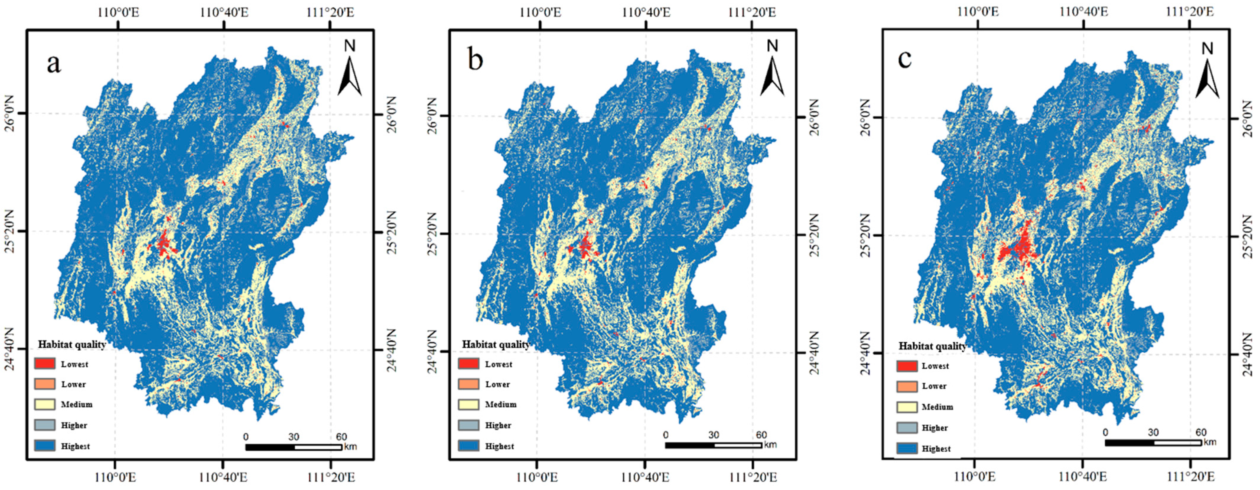
2.3.1. The HQ Assessment Based on the InVEST Model

The InVEST model assumes that biodiversity is proportional to HQ and evaluates the capacity and potential of ecosystems to support species survival, reproduction, and activity by calculating HQ [31,32]. HQ is directly related to habitat suitability provided by LUC types [33], evaluating both the intensity of external threats and ecosystem sensitivity. The calculation formula is as follows:
Q x j = H x j [ 1 ( D x j 2 D x j 2 + k 2 ) ]
where Qxj is the HQ of grid x in LUC-type j. Its value is between 0 and 1, and the higher the value, the better the HQ. Dxj is the habitat degradation degree of grid x in LUC-type j, ranging from 0 to 1. Hxj is the habitat suitability of x in LUC-type j, in which the suitability of the non-habitat LUC type is 0 and the suitability of the optimal habitat category is 1. k is the half-saturation constant.
In general, the suitability of natural landscapes is relatively high, while man-made landscapes are largely unsuitable [10]. Therefore, this study divided the habitat types into six categories based on the features of the study region and previous research [34,35,36]. WL and WTL were considered to be the LUC types with the highest habitat suitability for species, and their suitability values were set as 1 (Table 1).
D x j = r = 1 r y = 1 y ( w r n = 1 n w r ) r y i r x y β x S j r
where irxy is the impact of threat factor r in grid y on grid x; wr is the weight of different threat factors; ry indicates the intensity of the threat factor; and Sjr is the sensitivity of different habitats to different threat factors.
In a general sense, natural landscapes exhibit the highest sensitivity to threat factors, followed by semi-artificial landscapes and artificial landscapes, which are relatively less sensitive to threat factors with a certain degree of resistance to interference [37]. The sensitivity value spans from 0 to 1, where a score of 1 signifies the utmost sensitivity, while a score of 0 denotes no sensitivity. In addition, the higher the degree of human use of land species, the more serious the threat is to the habitat. CL is a notable expression of the alteration in the human natural environment, portraying the threat posed by human pressure to the natural ecosystem. As a semi-natural and semi-artificial environment, AL poses a certain degree of threat to the natural ecosystem [38]. Transport networks have cumulative and irreversible impacts on ecosystem services and biodiversity, and their construction leads to habitat fragmentation, thus becoming a serious threat [39]. Therefore, this study took CL, AL, and transportation land as threat factors. This study determined the sensitivity assignment of different habitat types (Table 1), the weight of threat factors, and the maximum impact distance of threat sources (Table 2) concerning the literature review and InVEST model manual and the specific conditions of the study area [40,41,42].

2.3.2. Landscape Structure Index

The greater the complexity of ecosystems, the better the state of the landscape structure, and the more balanced the categories within a given area, the greater the degree of landscape diversity [43]. Therefore, the state of landscape structure can indirectly reflect the strength of regional landscape diversity; calculating the landscape structure index in different periods enables a quantitative assessment of the changing state of regional landscape diversity. The landscape structure index highly condenses the information on LP, which is obtained by superimposing the weights of landscape fragmentation, landscape separation, and landscape fractal dimension [34]. The calculation formula is as follows:
L S I x = 1 ( a C i + b N i + c F i )
C i = n i A i
N i = 0.5 n i / A A A i
F i = 2 ln ( P i 4 ) ln A i
where LSIx is the landscape structure index; Ci is the landscape fragmentation index, expressing the degree of fragmentation of the entire landscape or a certain landscape type in a given nature; Ni is the landscape separation index, representing the dispersion degree of the spatial distribution of different patches in a landscape; Fi is the landscape fractal dimension, describing the complex characteristics of patch morphology in the landscape; Pi is the proportion of LUC-type i patches in the area; ni is the patch number of LUC-type i; Ai is the total area of LUC-type i. a, b, and c are the weights of each index and a + b + c = 1. The weights of landscape fragmentation, separation, and fractal dimensions 0.5, 0.3, and 0.2 were assigned, respectively, based on previous relevant research results [44,45].

2.3.3. Biodiversity Index

Ecological processes and landscape patterns interact, jointly influencing the quantity and distribution of species, and thus, indirectly affect the richness of biodiversity [46,47]. The biodiversity index was constructed from the ecosystem and landscape structure aspects by combining the natural and social conditions of Guilin in this study. The HQI and the landscape structure index were selected to comprehensively assess the level of biodiversity in the study area based on the research method of Sallustio et al. [48]. The calculation formula is as follows:
B I x = Q x j β 1 + L S I x β 2
where BIx is the comprehensive index of biodiversity; Qxj is the habitat quality of grid x; LSIx is the landscape structure index of grid x; and β is the weight value of each index. Considering that the whole of Guilin was mainly a mountainous forest area, the vegetation coverage rate was high, while the towns and populations were relatively concentrated in the downtown, and the landscape was relatively simple. Therefore, the impact of the habitat quality index was greater than the landscape structure index in the comprehensive assessment of biodiversity in Guilin, and the final weights of β1 and β2 were 0.6 and 0.4, respectively.
To more intuitively understand the status of regional indices and compare the differences between regional indices, the natural breakpoint method was used to divide them into the following five levels, highest, higher, medium, lower, and lowest, after obtaining the spatial distribution of habitat quality, landscape structure, and biodiversity in the study area. And the spatial change values of biodiversity were classified into three categories, decreasing, basically unchanged, and increasing, in which the change values between 0 and 5% were defined as basically unchanged.

2.3.4. Analysis of Biodiversity Hot and Cold Spots

Hotspot analysis can effectively identify special areas where biodiversity is seriously threatened, providing a scientific reference for the planning and management of biodiversity conservation in space [15,49]. This study selected hotspots and cold spots with confidence higher than 90% using ArcGIS software (v 10.6) to reflect the clustering distribution of high and low biodiversity values based on the Getis-Ord Gi* method. The formulas are as follows:
G i * = j = 1 n w i j x j X ¯ j = 1 n w i j S [ n j = 1 n w i j 2 ( j = 1 n w i j ) ] 2 n 1
X ¯ = j = 1 n x j n
S = j = 1 n x j 2 n 1 X ¯ 2
where xj is the attribute value of the spatial element j; wij is the spatial weight between elements i and j, which is defined as 1 for neighboring and 0 for non-neighboring; n is the total number of spatial elements; X ¯ is the mean of spatial elements; S is the standard deviation of spatial elements. G i * statistics are z-scores. The higher the z-scores, the closer the clustering of spatial elements with high values. The lower the z score, the closer the clustering of spatial elements with low values.

2.3.5. Future LUC Simulation Projections

The GeoSOS-FLUS model is a multi-class LUC change scenario simulation model developed by Liu et al. [50,51] based on the principle of the FLUS model. This is mainly composed of an artificial neural network and an adaptive inertia competition mechanism. The artificial neural network can effectively discover the relationship between natural, social, and economic factors and LUC change, obtaining the suitable probability of each class in the research scope. The adaptive inertial competition mechanism can help to solve the uncertainty of local class transformation and make up for the complexity of the local transformation and parameter determination of traditional cellular automata. The GeoSOS-FLUS model has better predictive power and higher accuracy compared with other models. Therefore, the GeoSOS-FLUS model was used to simulate and compare the LUC layout under the scenarios of NDS and EPS in Guilin in 2040, testing the effectiveness of biodiversity protection measures.
This study synthesized natural and socio-economic factors, selecting the DEM, slope, aspect, annual rainfall, GDP, and average annual temperature as the driving factors of LUC change. The probability, intensity, and direction of transitions between different LUC types were adjusted by setting the model parameters for different scenarios of the LUC simulation. (1) In the NDS, the Markov chain was applied to predict the LUC demand in 2040 according to the LUC transfer matrix from 2000 to 2020. The parameters of the model remained unchanged, and the trends in population, economic, and technological innovation continued to align with the current situation in this scenario. (2) In the EPS, WTL, and WL should be protected first, while CL and AL should be controlled based on the analysis results of the cold spots and hotspots of biodiversity in the study area. It is established that WL and WTL cannot be converted to other LUC types, and the neighboring factor of WL and WTL was set to 1. The neighboring factor of CL and AL was set to 0, and the neighboring factor of other LUC types was set to 0.5.

3. Results

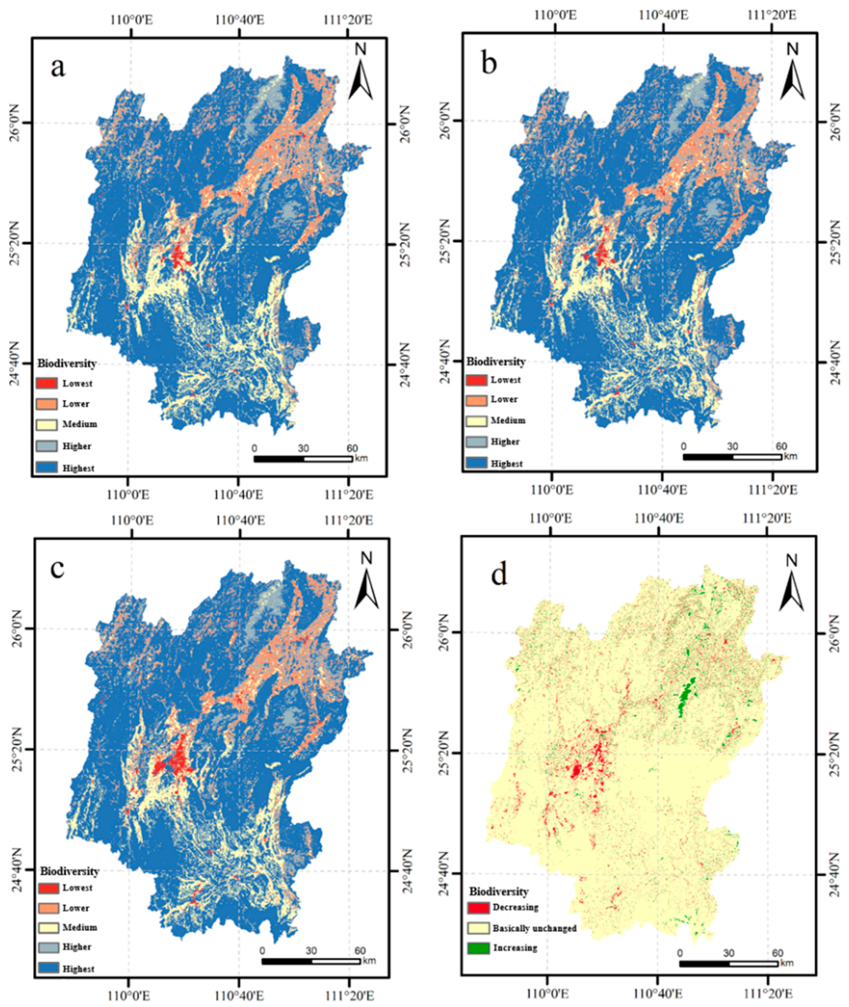
3.1. Analysis of Spatiotemporal Changes in Biodiversity

The spatiotemporal distribution characteristics of HQ (Figure 3) and landscape structure (Figure 4) from 2000 to 2020 showed a certain pattern. The average annual value of HQI decreased from 0.847 in 2000 to 0.841 in 2020. The low values were concentrated in urban areas and towns in the central part of the country, with the lowest HQI being 0. The high-value areas were mainly distributed in the surrounding mountainous forest area, and the HQI was higher than 0.8. There was a small decrease in the landscape structure index from 2000 to 2020, with the annual average value decreasing from 0.921 to 0.918. The landscape structure index decreased gradually from the southwest to the northeast. The LUC types in low-value areas were complex and diverse, and the landscape fragmentation was high. The high-value area was mainly forestland with good natural and ecological conditions.
The annual average value of the biodiversity index decreased from 0.875 to 0.870. The proportion of the area in high-value areas shrank from 68.53% to 68.22% and increased from 0.85% to 1.81% in the low-value areas from 2000 to 2020. The overall spatial distribution characteristics of biodiversity were “higher in the northwest, southwest, and east, and lower in the northeast, southeast, and central” (Figure 5). Low-value areas were widely distributed in construction land, arable land, and interspersed areas of various LUC types, including mainly the city center, Lingchuan County, Xing’an County, and Quanzhou County, with the lowest biodiversity index of 0.13. The median-value areas were primarily concentrated on southern arable land, including Lingui District, Yangshuo County, Lipu City, Pingle County, and Gongcheng County. High-value areas were primarily concentrated in mountainous forest areas, including Longsheng County, Ziyuan County, Yongfu County, and Guanyang County. The biodiversity index was higher than 0.9. The area of biodiversity reduction was 4.1% and primarily distributed in the surrounding areas of cities and towns. The increasing area of biodiversity accounted for 3.13% and was primarily concentrated in grassland and forest areas.

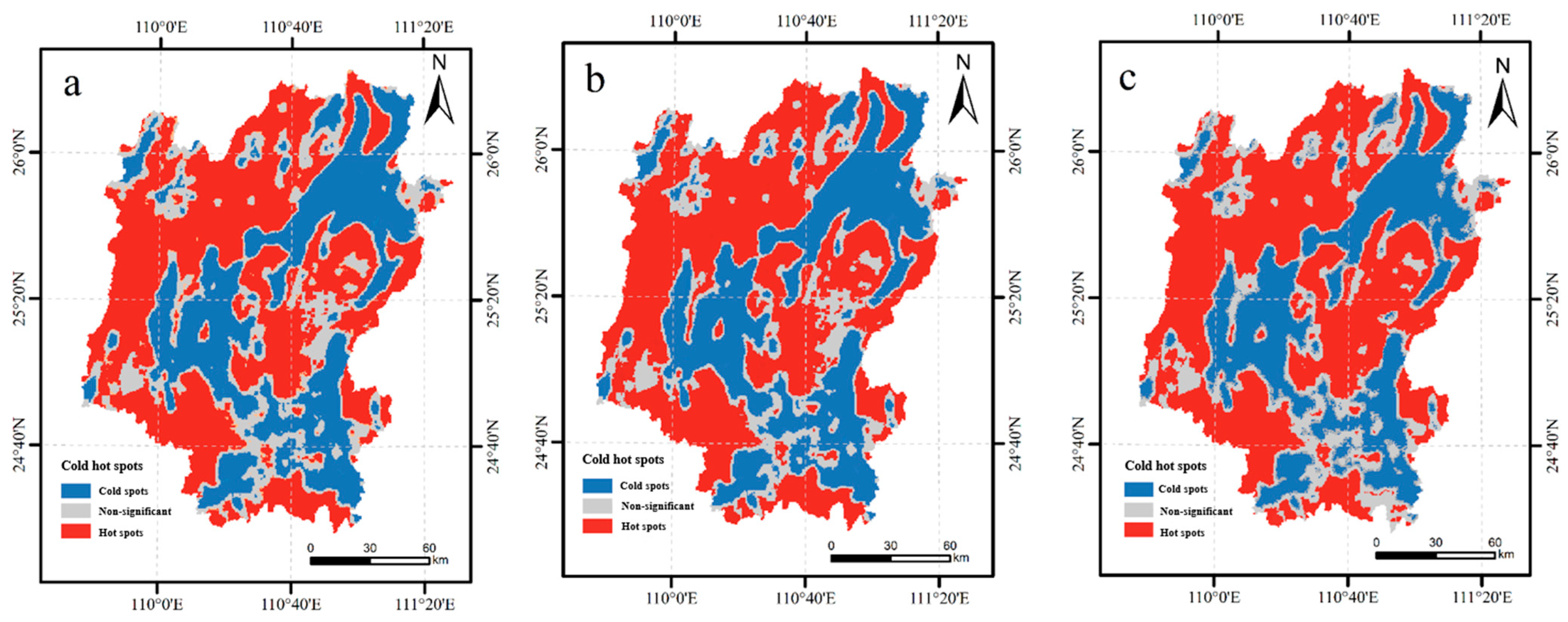
3.2. Analysis of Cold and Hot Spots of Biodiversity from 2000 to 2020

The spatiotemporal distribution of cold and hot spots of biodiversity in Guilin showed significant differences (Figure 6). The total area of hotspots showed a slightly increasing trend, increasing from 49.65% to 50.56% from 2000 to 2020. The biodiversity hotspots were discontinuous and distributed in Longsheng County, Ziyuan County, Yongfu County, and Guanyang County, many of which were divided by cold spots. The area proportion of the cold spots decreased from 31.16% to 30.54%, with a slightly decreasing trend. The cold spots of biodiversity were scattered, primarily concentrated in the city center, Quanzhou County, and Pingle County, with scattering in other areas.
The coverage of cold and hot spots of biodiversity exhibited significant variation among the different LUC types from 2000 to 2020 (Table 3). The coverage rate of hotspots was the highest in WTL (94.45%), followed by AL (64.19%) among the LUC types. The coverage of hotspots in GL and WT was low, with the highest reaching 40.19%. The coverage of hotspots in CL and AL was lower than 13.37%. The CL (91.67%), followed by AL (70.08%), had the highest coverage rate of cold spots over the past 20 years, which was mainly composed of WL with a coverage rate of 89.7%. The cold spot coverage of GL and WT was low, with a maximum of 51.74%. The cold spot coverage of WL and WTL was below 17.24% for both. The cold spot areas mainly consisted of AL, with a coverage rate of about 51.11%.

3.3. Comparison of Biodiversity in Different Scenarios in 2040

The biodiversity of Guilin showed an opposite changing trend under two scenarios. The projected annual mean value of the biodiversity index in 2040 was 0.859, with a decrease of 1.26% from 2020 in the NDS (Figure 7a). The predicted annual mean biodiversity index in 2040 was 0.872, with an increase of 0.22% compared with 2020 in the EPS (Figure 7b). The proportion of biodiversity at all levels in the EPS changed significantly compared to the NDS. The highest proportion of the regional area was the highest-value areas (67.33%), followed by the middle-value areas, lower-value areas, and higher-value areas, accounting for 16.03%, 8.6%, and 5.33% in the NDS, respectively. The lowest proportion of low-value areas was only 3.25%. The highest proportion of the regional area was the highest-value areas (67.52%), which increased by 0.19% compared with the NDS. This was followed by the medium, higher-value areas, and lower-value areas, which accounted for 15.15%, 8.23%, and 7.22%, respectively, while the proportion of lowest-value areas decreased significantly to only 1.89%.
The spatial pattern of biodiversity in 2040 exhibited no clear change under the two scenarios. It still presented a higher distribution in the northwest, southwest, and east and a lower distribution in the northeast, southeast, and central. The biodiversity reduction area under the NDS (Figure 7c) accounted for 4.15% of the entire area of Guilin, primarily concentrated in the urban expansion zone. The biodiversity increase area in the EPS (Figure 7d) accounted for 5.67% of the whole area of Guilin and was widely distributed in the grassland and forest areas. The biodiversity reduction area accounted for 4.11% of the whole area of Guilin and was scattered in the surrounding areas of cities and farming zones. The biodiversity increase area accounted for 8.31% of the whole area of Guilin, with a 2.64% increase compared to the NDS, and was distributed in grassland and forest areas.

4. Discussion

4.1. Analysis of Biodiversity Change

Biodiversity serves as a crucial indicator of the overall health and sustainability of regional ecosystems [27]. It is integral to ecosystems and closely linked to human survival and well-being. Recently, the progress of urbanization has not only heightened human–land conflicts and altered LUC patterns but has also exerted a substantial impact on biodiversity [20,52]. Research has demonstrated that the combined use of HQ and LP can comprehensively assess biodiversity changes resulting from LUC alterations, offering novel perspectives and methodologies for biodiversity research.
The results of the study on biodiversity in Guilin showed that the overall situation of biodiversity has been good over the past 20 years. The annual average value of the biodiversity index exceeded 0.8, and most of the area belonged to the high-value areas of biodiversity (Figure 5). This was because LUC types in Guilin were dominated by WL, with high forest vegetation cover, a favorable regional ecological environment, and high species richness. In addition, the pillar industry of economic development is tourism in Guilin. The relevant departments pay more attention to ecological protection, while there are fewer heavy industries and less impact from human activities [53]. The spatial distribution characteristics of biodiversity showed a certain regularity. The low-value areas of biodiversity were primarily concentrated in urban and rural settlement areas and agricultural planting areas, where human activities were more frequent and agricultural cultivation was more developed. Regional landscape fragmentation was higher. The high-value areas were primarily distributed in mountain forests and lake wetlands, with high regional vegetation coverage, including nature reserves and parks with less surface disturbance. This was similar to the results of other studies in Guangxi [31,34,40]. The results also indicated that there was a decreasing trend of biodiversity in Guilin from 2000 to 2020, and the areas of biodiversity reduction were primarily concentrated around towns (Figure 5d). In recent years, the surrounding areas of cities have begun to assume part of the urban LUC function with the rapid advancement of urbanization. Artificial landscape elements have also begun to spread to the surrounding areas from a high concentration. The intrusion of various artificial landscapes seriously threatens the surrounding habitats, resulting in worsening landscape fragmentation and HQ deterioration in these areas. The steady development of biodiversity in the surrounding areas is, therefore, something that the Guilin government has to focus on more.

4.2. Impacts of Different Development Scenarios on Biodiversity

The analysis of the aggregation characteristics of biodiversity and its relationship with different LUC types can provide a comprehensive understanding of the sustainable study of biodiversity in Guilin [54]. This study took the hotspot areas as the priority protection areas for future development according to the analysis results of hot and cold spots, and more targeted ecological protection measures can be designed based on this. The coverage and contribution of hotspots in Guilin showed that WTL and WL are the main LUC types in biodiversity hotspots, while CL and AL were the main LUC types in the cold spots. Therefore, this study established the ecological protection strategy of “prioritizing the protection of WTL and WL, and rationally controlling CL and AL” to guarantee the priority of hotspot areas. It was found that regional biodiversity increased significantly under the protection measures by simulating and comparing the biodiversity of Guilin in 2040 under the scenarios of NDS and EPS. Compared with the NDS, the EPS adjusted the LUC structure. On the one hand, the protection of WTL and WL was strengthened, and the area with a high value of biodiversity increased significantly. On the other hand, low biodiversity value areas decreased by limiting the expansion of land for CL and AL. This was especially true since the rate of degradation in urban centers eased, and the proportion of areas with reduced biodiversity declined. The four key land types of WTL, WL, CL, and AL were targeted in the EPS, resulting in a synchronized expansion of biodiversity enhancement zones, a reduction in biodiversity decline zones, and a significant improvement in regional biodiversity.
WL and WTL are the key LUC types to maintain the stability of biodiversity in Guilin, and they are widely distributed around towns and cities. However, urban land and arable land continue to erode the ecological land such as WL and WTL, with the acceleration of the urbanization process in Guilin posing a challenge to the conservation of biodiversity [55]. Therefore, land managers and planners should balance the relationship between urban expansion and ecological protection, avoiding areas with high biodiversity as much as possible in the process of urban development [29]. WL and WTL resources should be actively protected to prevent the loss of biodiversity by improving the legal system of ecological protection and increasing the area of urban green space.

4.3. Limitations of the Study and Future Perspectives

Biodiversity conservation has been one of the hot topics in ecological service research in recent years. Therefore, developing effective methods for measuring biodiversity has remained a crucial and challenging issue [56]. Changes in plant diversity represent one of the consequences of landscape fragmentation and habitat change and are closely linked to LUC changes [30]. This study combined the landscape structure index and HQI to form a comprehensive biodiversity index, facilitating the assessment of spatiotemporal changes in plant biodiversity on a regional scale [57]. However, it is important to note that certain issues, such as the assessment of animal biodiversity, have not been thoroughly explored. Future studies should comprehensively consider the distribution of animals in the study area, conduct a thorough assessment of animal diversity indices and changes in plant diversity characteristics, and engage in multi-scale, multi-level, and multi-faceted biodiversity research.
The potential impacts of LUC modeling on biodiversity depend heavily on the accuracy of the predicted LUC data [58]. In this study, the GeoSOS-FLUS model was employed to simulate future LUC changes under different scenarios. Although it combined natural and socioeconomic factors and had high simulation accuracy, this model relied on the prediction of LUC demand. Additionally, the Markov chain only provided a simple description of future change trends based on historical data [59]. Furthermore, the impact of model parameter settings, spatial scales, and social policy changes on the outcomes were not considered in the applications. Furthermore, the applications did not account for the impact of model parameter settings, spatial scales, and social policy changes on the outcomes. Therefore, the predicted results may not perfectly align with the actual situation in 2040, but they can reveal certain characteristics and change mechanisms in LUC, providing a reference basis for government decision making [60].
For the HQ assessment using the InVEST model, parameters such as the maximum impact distance, threat source weight, and habitat sensitivity were primarily drawn from previous studies in similar regions. The setting of these parameters was somewhat subjective, potentially influencing the HQ evaluation results. Further research is needed to establish more reasonable guidelines for setting input parameters in the habitat quality model. In future studies, it is crucial to enhance continuous field monitoring to collect relevant data, thereby improving the capacity to interpret real-time habitat quality.

5. Conclusions

In this study, the InVEST model, GeoSOS-FLUS model, and landscape pattern index were combined to construct a comprehensive biodiversity index, which quantitatively assesses the spatiotemporal change characteristics of biodiversity in Guilin from 2000 to 2020. The effectiveness of the conservation measures was examined by comparing the simulation results of different scenarios in the future. The conclusions are as follows:
(1)
The overall biodiversity situation in Guilin exhibited a positive trajectory from 2000 to 2020. However, it also displayed a gradual decline, with an annual average biodiversity index decreasing from 0.875 to 0.870. The spatial distribution of biodiversity was differentiated, with the overall distribution characterized by “higher in the northwest, southwest, and east, and lower in the northeast, southeast, and central parts of the country”.
(2)
The biodiversity hotspots area was distributed in discontinuous patches in the northwestern, southwestern, and eastern parts of Guilin. The total area showed a slightly increasing trend from 2000 to 2020. Ecological protection measures have designated biodiversity hotspots as priority areas for protection, with emphasis on the protection of WTL and WL and the reasonable control of CL and AL.
(3)
The annual mean value of the biodiversity index of Guilin in the EPS in 2040 showed an upward trend compared with the NDS. It expanded the proportion of the area with high biodiversity value and effectively slowed down the degradation rate of regional biodiversity. The implementation of ecological protection measures can better achieve the goal of the sustainable development of biodiversity in Guilin and ensure regional ecological security.
In future development, it is crucial to prioritize the protection of vital ecological environments like mountains, water bodies, and wetlands. Human disturbance in these areas should be minimized, and measures such as afforestation and wetland restoration should be implemented.

Author Contributions

Conceptualization, Y.L.; methodology, Y.L. and K.Z.; validation, K.Z. and X.H.; formal analysis, M.L.; resources, Z.C., M.L., H.Y. and X.H.; data curation, Y.L.; writing—original draft preparation, Y.L.; writing—review and editing, Y.L. and K.Z.; visualization, Y.L.; supervision, K.Z., X.H., Z.C., J.C. and M.L.; funding acquisition, J.C., Z.C., H.Y., X.H. and M.L. All authors have read and agreed to the published version of the manuscript.

Funding

This study was supported by grants from the Major Special Projects of the High-Resolution Earth Observation System (84-Y50G25-9001-22/23), the Guangxi Natural Science Foundation (2021GXNSFBA220001), and the Guangxi Key Laboratory of Spatial Information and Geomatics under grant (19-050-11-22).

Institutional Review Board Statement

Not applicable.

Informed Consent Statement

Not applicable.

Data Availability Statement

Data are contained within the article.

Acknowledgments

The authors sincerely thank the editors and the anonymous reviewers for their constructive feedback.

Conflicts of Interest

The authors declare no conflicts of interest.

References

  1. Jaureguiberry, P.; Titeux, N.; Wiemers, M.; Bowler, D.E.; Coscieme, L.; Golden, A.S.; Guerra, C.A.; Jacob, U.; Takahashi, Y.; Settele, J.; et al. The direct drivers of recent global anthropogenic biodiversity loss. Sci. Adv. 2022, 8, eabm9982. [Google Scholar] [CrossRef]
  2. Isbell, F.; Reich, P.B.; Tilman, D.; Hobbie, S.E.; Polasky, S.; Binder, S. Nutrient enrichment, biodiversity loss, and consequent declines in ecosystem productivity. Proc. Natl. Acad. Sci. USA 2013, 110, 11911–11916. [Google Scholar] [CrossRef]
  3. Chaplin-Kramer, R.; Sharp, R.P.; Mandle, L.; Sim, S.; Johnson, J.; Butnar, I.; Milà i Canals, L.; Eichelberger, B.A.; Ramler, I.; Mueller, C.; et al. Spatial patterns of agricultural expansion determine impacts on biodiversity and carbon storage. Proc. Natl. Acad. Sci. USA 2015, 112, 7402–7407. [Google Scholar] [CrossRef]
  4. Sharma, R.; Nehren, U.; Rahman, S.A.; Meyer, M.; Rimal, B.; Aria Seta, G.; Baral, H. Modeling Land Use and Land Cover Changes and Their Effects on Biodiversity in Central Kalimantan, Indonesia. Land 2018, 7, 57. [Google Scholar] [CrossRef]
  5. Yu, Y.; Li, J.; Zhou, Z.; Ma, X.; Zhang, X. Response of multiple mountain ecosystem services on environmental gradients: How to respond, and where should be priority conservation? J. Clean. Prod. 2021, 278, 123264. [Google Scholar] [CrossRef]
  6. Newbold, T.; Hudson, L.N.; Hill, S.L.L.; Contu, S.; Lysenko, I.; Senior, R.A.; Börger, L.; Bennett, D.J.; Choimes, A.; Collen, B.; et al. Global effects of land use on local terrestrial biodiversity. Nature 2015, 520, 45–50. [Google Scholar] [CrossRef]
  7. Suo, A.; Wang, C.; Zhang, M. Analysis of sea use landscape pattern based on GIS: A case study in Huludao, China. SpringerPlus 2016, 5, 1587. [Google Scholar] [CrossRef]
  8. Cegielska, K.; Noszczyk, T.; Kukulska, A.; Szylar, M.; Hernik, J.; Dixon-Gough, R.; Jombach, S.; Valánszki, I.; Filepné Kovács, K. Land use and land cover changes in post-socialist countries: Some observations from Hungary and Poland. Land Use Policy 2018, 78, 1–18. [Google Scholar] [CrossRef]
  9. Janus, J.; Taszakowski, J. Spatial differentiation of indicators presenting selected barriers in the productivity of agricultural areas: A regional approach to setting land consolidation priorities. Ecol. Indic. 2018, 93, 718–729. [Google Scholar] [CrossRef]
  10. Terrado, M.; Sabater, S.; Chaplin-Kramer, B.; Mandle, L.; Ziv, G.; Acuña, V. Model development for the assessment of terrestrial and aquatic habitat quality in conservation planning. Sci. Total Environ. 2016, 540, 63–70. [Google Scholar] [CrossRef]
  11. Wang, Y.; Dai, E. Spatial-temporal changes in ecosystem services and the trade-off relationship in mountain regions: A case study of Hengduan Mountain region in Southwest China. J. Clean. Prod. 2020, 264, 121573. [Google Scholar] [CrossRef]
  12. Hao, R.; Yu, D.; Wu, J. Relationship between paired ecosystem services in the grassland and agro-pastoral transitional zone of China using the constraint line method. Agric. Ecosyst. Environ. 2017, 240, 171–181. [Google Scholar] [CrossRef]
  13. Janus, J.; Bozek, P. Land abandonment in Poland after the collapse of socialism: Over a quarter of a century of increasing tree cover on agricultural land. Ecol. Eng. 2019, 138, 106–117. [Google Scholar] [CrossRef]
  14. Zhang, Y.; Chen, R.; Wang, Y. Tendency of land reclamation in coastal areas of Shanghai from 1998 to 2015. Land Use Policy 2020, 91, 104370. [Google Scholar] [CrossRef]
  15. Liu, Y.; Huang, X.; Yang, H.; Zhong, T. Environmental effects of land-use/cover change caused by urbanization and policies in Southwest China Karst area—A case study of Guiyang. Habitat Int. 2014, 44, 339–348. [Google Scholar] [CrossRef]
  16. Ling, M.; Chen, J.; Lan, Y.; Chen, Z.; You, H.; Han, X.; Zhou, G. Exploring the Drivers of Soil Conservation Variation in the Source of Yellow River under Diverse Development Scenarios from a Geospatial Perspective. Sustainability 2024, 16, 777. [Google Scholar] [CrossRef]
  17. Chen, X.; He, X.; Wang, S. Simulated Validation and Prediction of Land Use under Multiple Scenarios in Daxing District, Beijing, China, Based on GeoSOS-FLUS Model. Sustainability 2022, 14, 11428. [Google Scholar] [CrossRef]
  18. Wang, J.; Lv, J.; Zhang, W.; Chen, T.; Yang, Y.; Wu, J. Land-Use Pattern Evaluation Using GeoSOS-FLUS in National Territory Spatial Planning: A Case Study of Changzhi City, Shanxi Province. Sustainability 2022, 14, 13752. [Google Scholar] [CrossRef]
  19. Wang, Y.; Shen, J.; Yan, W.; Chen, C. Backcasting approach with multi-scenario simulation for assessing effects of land use policy using GeoSOS-FLUS software. MethodsX 2019, 6, 1384–1397. [Google Scholar] [CrossRef]
  20. Zhou, Q.; van den Bosch, C.C.K.; Chen, J.; Zhang, W.; Dong, J. Identification of ecological networks and nodes in Fujian province based on green and blue corridors. Sci. Rep. 2021, 11, 20872. [Google Scholar] [CrossRef]
  21. Upadhaya, S.; Dwivedi, P. Conversion of forestlands to blueberries: Assessing implications for habitat quality in Alabaha river watershed in Southeastern Georgia, United States. Land Use Policy 2019, 89, 104229. [Google Scholar] [CrossRef]
  22. Wu, C.-F.; Lin, Y.-P.; Chiang, L.-C.; Huang, T. Assessing highway’s impacts on landscape patterns and ecosystem services: A case study in Puli Township, Taiwan. Landsc. Urban Plan. 2014, 128, 60–71. [Google Scholar] [CrossRef]
  23. Zhang, D.; Wang, X.; Qu, L.; Li, S.; Lin, Y.; Yao, R.; Zhou, X.; Li, J. Land use/cover predictions incorporating ecological security for the Yangtze River Delta region, China. Ecol. Indic. 2020, 119, 106841. [Google Scholar] [CrossRef]
  24. Ricketts, T.H.; Lonsdorf, E. Mapping the margin: Comparing marginal values of tropical forest remnants for pollination services. Ecol. Appl. 2013, 23, 1113–1123. [Google Scholar] [CrossRef] [PubMed]
  25. Tang, Y.; Gao, C.; Wu, X. Urban Ecological Corridor Network Construction: An Integration of the Least Cost Path Model and the InVEST Model. ISPRS Int. J. Geo-Inf. 2020, 9, 33. [Google Scholar] [CrossRef]
  26. Gong, J.; Xie, Y.C.; Cao, E.J.; Huang, Q.Y.; Li, H.Y. Integration of InVEST-habitat quality model with landscape pattern indexes to assess mountain plant biodiversity change: A case study of Bailongjiang watershed in Gansu Province. J. Geogr. Sci. 2019, 29, 1193–1210. [Google Scholar] [CrossRef]
  27. Wei, P.; Chen, S.; Wu, M.; Deng, Y.; Xu, H.; Jia, Y.; Liu, F. Using the InVEST Model to Assess the Impacts of Climate and Land Use Changes on Water Yield in the Upstream Regions of the Shule River Basin. Water 2021, 13, 1250. [Google Scholar] [CrossRef]
  28. Wang, D.; Hu, M.; Tang, X.; Zhang, Q.; Zhao, J.; Mao, B.; Zhang, H.; Cui, S. Characterization of physicochemical properties and flavor profiles of fermented Chinese bamboo shoots (suansun) from Liuzhou and Guilin. Food Biosci. 2023, 56, 103125. [Google Scholar] [CrossRef]
  29. Li, F.; Wang, L.; Chen, Z.; Clarke, K.C.; Li, M.; Jiang, P. Extending the SLEUTH model to integrate habitat quality into urban growth simulation. J. Environ. Manag. 2018, 217, 486–498. [Google Scholar] [CrossRef]
  30. Yang, Y.; Chen, J.; Lan, Y.; Zhou, G.; You, H.; Han, X.; Wang, Y.; Shi, X. Landscape Pattern and Ecological Risk Assessment in Guangxi Based on Land Use Change. Int. J. Environ. Res. Public Health 2022, 19, 1595. [Google Scholar] [CrossRef]
  31. Mirghaed, F.A.; Mohammadzadeh, M.; Salmanmahiny, A.; Mirkarimi, S.H. Decision scenarios using ecosystem services for land allocation optimization across Gharehsoo watershed in northern Iran. Ecol. Indic. 2020, 117, 106645. [Google Scholar] [CrossRef]
  32. Sharma, R.; Rimal, B.; Stork, N.; Baral, H.; Dhakal, M. Spatial Assessment of the Potential Impact of Infrastructure Development on Biodiversity Conservation in Lowland Nepal. ISPRS Int. J. Geo-Inf. 2018, 7, 365. [Google Scholar] [CrossRef]
  33. Dwiningsih, Y. Utilizing the Genetic Potentials of Traditional Rice Varieties and Conserving Rice Biodiversity with System of Rice Intensification Management. Agronomy 2023, 13, 3015. [Google Scholar] [CrossRef]
  34. Wilson, M.C.; Chen, X.Y.; Corlett, R.T.; Didham, R.K.; Ding, P.; Holt, R.D.; Holyoak, M.; Hu, G.; Hughes, A.C.; Jiang, L.; et al. Habitat fragmentation and biodiversity conservation: Key findings and future challenges. Landsc. Ecol. 2016, 31, 229–230. [Google Scholar] [CrossRef]
  35. Mengist, W.; Soromessa, T.; Legese Feyisa, G. Responses of soil and water-related ecosystem services to landscape dynamics in the eastern Afromontane biodiversity Hotspot. Heliyon 2023, 9, e22639. [Google Scholar] [CrossRef]
  36. Tang, F.; Fu, M.C.; Wang, L.; Zhang, P.T. Land-use change in Changli County, China: Predicting its spatio-temporal evolution in habitat quality. Ecol. Indic. 2020, 117, 106719. [Google Scholar] [CrossRef]
  37. Sun, X.Y.; Jiang, Z.; Liu, F.; Zhang, D.Z. Monitoring spatio-temporal dynamics of habitat quality in Nansihu Lake basin, eastern China, from 1980 to 2015. Ecol. Indic. 2019, 102, 716–723. [Google Scholar] [CrossRef]
  38. Yang, Y.Y. Evolution of habitat quality and association with land-use changes in mountainous areas: A case study of the Taihang Mountains in Hebei Province, China. Ecol. Indic. 2021, 129, 107967. [Google Scholar] [CrossRef]
  39. Zhang, H.; Zhang, C.; Hu, T.; Zhang, M.; Ren, X.W.; Hou, L. Exploration of roadway factors and habitat quality using InVEST. Transp. Res. Part D-Transp. Environ. 2020, 87, 102551. [Google Scholar] [CrossRef]
  40. Xiong, K.; He, C.; Chi, Y. Research Progress on Grassland Eco-Assets and Eco-Products and Its Implications for the Enhancement of Ecosystem Service Function of Karst Desertification Control. Agronomy 2023, 13, 2394. [Google Scholar] [CrossRef]
  41. Qiao, X.; Li, Z.; Lin, J.; Wang, H.; Zheng, S.; Yang, S. Assessing current and future soil erosion under changing land use based on InVEST and FLUS models in the Yihe River Basin, North China. Int. Soil Water Conserv. Res. 2023, 7, 1–15. [Google Scholar] [CrossRef]
  42. Balbi, M.; Petit, E.J.; Croci, S.; Nabucet, J.; Georges, R.; Madec, L.; Ernoult, A. Title: Ecological relevance of least cost path analysis: An easy implementation method for landscape urban planning. J. Environ. Manag. 2019, 244, 61–68. [Google Scholar] [CrossRef]
  43. Xu, X.; Yang, G.; Tan, Y.; Liu, J.; Hu, H. Ecosystem services trade-offs and determinants in China’s Yangtze River Economic Belt from 2000 to 2015. Sci. Total Environ. 2018, 634, 1601–1614. [Google Scholar] [CrossRef]
  44. He, L.; Xie, Z.; Wu, H.; Liu, Z.; Zheng, B.; Wan, W. Exploring the interrelations and driving factors among typical ecosystem services in the Yangtze river economic Belt, China. J. Environ. Manag. 2024, 351, 119794. [Google Scholar] [CrossRef]
  45. Gao, Y.; Ma, L.; Liu, J.; Zhuang, Z.; Huang, Q.; Li, M. Constructing Ecological Networks Based on Habitat Quality Assessment: A Case Study of Changzhou, China. Sci. Rep. 2017, 7, 46073. [Google Scholar] [CrossRef]
  46. Kienast, F.; Walters, G.; Bürgi, M. Landscape ecology reaching out. Landsc. Ecol. 2021, 36, 2189–2198. [Google Scholar] [CrossRef]
  47. Nie, W.; Shi, Y.; Siaw, M.J.; Yang, F.; Wu, R.; Wu, X.; Zheng, X.; Bao, Z. Constructing and optimizing ecological network at county and town Scale: The case of Anji County, China. Ecol. Indic. 2021, 132, 108294. [Google Scholar] [CrossRef]
  48. Sallustio, L.; De Toni, A.; Strollo, A.; Di Febbraro, M.; Gissi, E.; Casella, L.; Geneletti, D.; Munafò, M.; Vizzarri, M.; Marchetti, M. Assessing habitat quality in relation to the spatial distribution of protected areas in Italy. J. Environ. Manag. 2017, 201, 129–137. [Google Scholar] [CrossRef]
  49. Reyers, B.; O’Farrell, P.J.; Cowling, R.M.; Egoh, B.N.; Le Maitre, D.C.; Vlok, J.H.J. Ecosystem Services, Land-Cover Change, and Stakeholders: Finding a Sustainable Foothold for a Semiarid Biodiversity Hotspot. Ecol. Soc. 2009, 14, 23. [Google Scholar] [CrossRef]
  50. Huang, X.; Ye, Y.; Zhao, X.; Guo, X.; Ding, H. Identification and stability analysis of critical ecological land: Case study of a hilly county in southern China. Ecol. Indic. 2022, 141, 109091. [Google Scholar] [CrossRef]
  51. Liu, X.P.; Liang, X.; Li, X.; Xu, X.C.; Ou, J.P.; Chen, Y.M.; Li, S.Y.; Wang, S.J.; Pei, F.S. A future land use simulation model (FLUS) for simulating multiple land use scenarios by coupling human and natural effects. Landsc. Urban Plan. 2017, 168, 94–116. [Google Scholar] [CrossRef]
  52. Zhang, R.; Pu, L.; Li, J.; Zhang, J.; Xu, Y. Landscape ecological security response to land use change in the tidal flat reclamation zone, China. Environ. Monit. Assess. 2015, 188, 1. [Google Scholar] [CrossRef] [PubMed]
  53. Zhang, X.; Song, W.; Lang, Y.; Feng, X.; Yuan, Q.; Wang, J. Land use changes in the coastal zone of China’s Hebei Province and the corresponding impacts on habitat quality. Land Use Policy 2020, 99, 104957. [Google Scholar] [CrossRef]
  54. Bai, L.; Xiu, C.; Feng, X.; Liu, D. Influence of urbanization on regional habitat quality:a case study of Changchun City. Habitat Int. 2019, 93, 102042. [Google Scholar] [CrossRef]
  55. Chen, J.; Yang, Y.; Feng, Z.; Huang, R.; Zhou, G.; You, H.; Han, X. Ecological Risk Assessment and Prediction Based on Scale Optimization—A Case Study of Nanning, a Landscape Garden City in China. Remote Sens. 2023, 15, 1304. [Google Scholar] [CrossRef]
  56. Rosa, I.M.D.; Purvis, A.; Alkemade, R.; Chaplin-Kramer, R.; Ferrier, S.; Guerra, C.A.; Hurtt, G.; Kim, H.; Leadley, P.; Martins, I.S.; et al. Challenges in producing policy-relevant global scenarios of biodiversity and ecosystem services. Glob. Ecol. Conserv. 2020, 22, e00886. [Google Scholar] [CrossRef]
  57. Cong, P.; Chen, K.; Qu, L.; Han, J. Dynamic Changes in the Wetland Landscape Pattern of the Yellow River Delta from 1976 to 2016 Based on Satellite Data. Chin. Geogr. Sci. 2019, 29, 372–381. [Google Scholar] [CrossRef]
  58. Weng, Q.H. Land use change analysis in the Zhujiang Delta of China using satellite remote sensing, GIS and stochastic modelling. J. Environ. Manag. 2002, 64, 273–284. [Google Scholar] [CrossRef]
  59. Zhao, J.; Shao, Z.; Xia, C.Y.; Fang, K.; Chen, R.; Zhou, J. Ecosystem services assessment based on land use simulation: A case study in the Heihe River Basin, China. Ecol. Indic. 2022, 143, 109402. [Google Scholar] [CrossRef]
  60. Xu, L.; Chen, S.S.; Xu, Y.; Li, G.; Su, W. Impacts of Land-Use Change on Habitat Quality during 1985–2015 in the Taihu Lake Basin. Sustainability 2019, 11, 3513. [Google Scholar] [CrossRef]
Figure 1. The spatial distribution of land use in Guilin.
Applsci 14 02101 g001
Figure 2. The framework of this study.
Applsci 14 02101 g002
Figure 3. Spatial distribution of habitat quality. ((a): 2000; (b): 2010; and (c): 2020).
Applsci 14 02101 g003
Figure 4. Spatial distribution of landscape structure. ((a): 2000; (b): 2010; and (c): 2020).
Applsci 14 02101 g004
Figure 5. Spatial distribution and change in biodiversity. ((a): 2000; (b): 2010; (c): 2020; and (d): the spatial change in biodiversity from 2000 to 2020).
Applsci 14 02101 g005
Figure 6. Distribution of biodiversity cold and hot spots. ((a): 2000; (b): 2010; and (c): 2020).
Applsci 14 02101 g006
Figure 7. Spatial distribution and change in biodiversity in 2040. ((a): NDS; (b): EPS; (c): the spatial changes in biodiversity under NDS; and (d): the spatial changes in biodiversity under ESP).
Applsci 14 02101 g007
Table 1. Evaluation of habitat suitability and its relative sensitivity to different threat sources.
LULCName *HabitatL_ALL_CL
1AL0.400.6
2WL10.750.9
3GL0.80.450.7
4WTL10.70.85
5WT0.90.30.75
6CL000
*: AL (arable land), WL (woodland), GL (grassland), WTL (wetland), WT (waters), CL (construction land).
Table 2. Threat factors, maximum threat distance, weight and attenuation type.
Threat FactorsMax_DistWeightDecay
Arable land1.50.5linear
Construction land5.50.9linear
Railway2.50.6linear
Highway1.50.5linear
Table 3. Biodiversity cold and hot spots with coverage of different LUC types in 2000 and 2020.
Type *Hot Spots (%)Cold Spots (%)
2000202020002020
AL13.3713.3771.3068.86
WL64.1964.1917.2416.51
GL40.1940.1937.8136.73
WTL100.0088.890.0011.11
WT32.6832.6851.5851.74
CL3.373.3792.4790.87
*: AL (arable land), WL (woodland), GL (grassland), WTL (wetland), WT (waters), CL (construction land).
Disclaimer/Publisher’s Note: The statements, opinions and data contained in all publications are solely those of the individual author(s) and contributor(s) and not of MDPI and/or the editor(s). MDPI and/or the editor(s) disclaim responsibility for any injury to people or property resulting from any ideas, methods, instructions or products referred to in the content.

