
A New Approach for Discontinuity Extraction Based on an Improved Naive Bayes Classifier

 ,
,
Abstract
1. Introduction
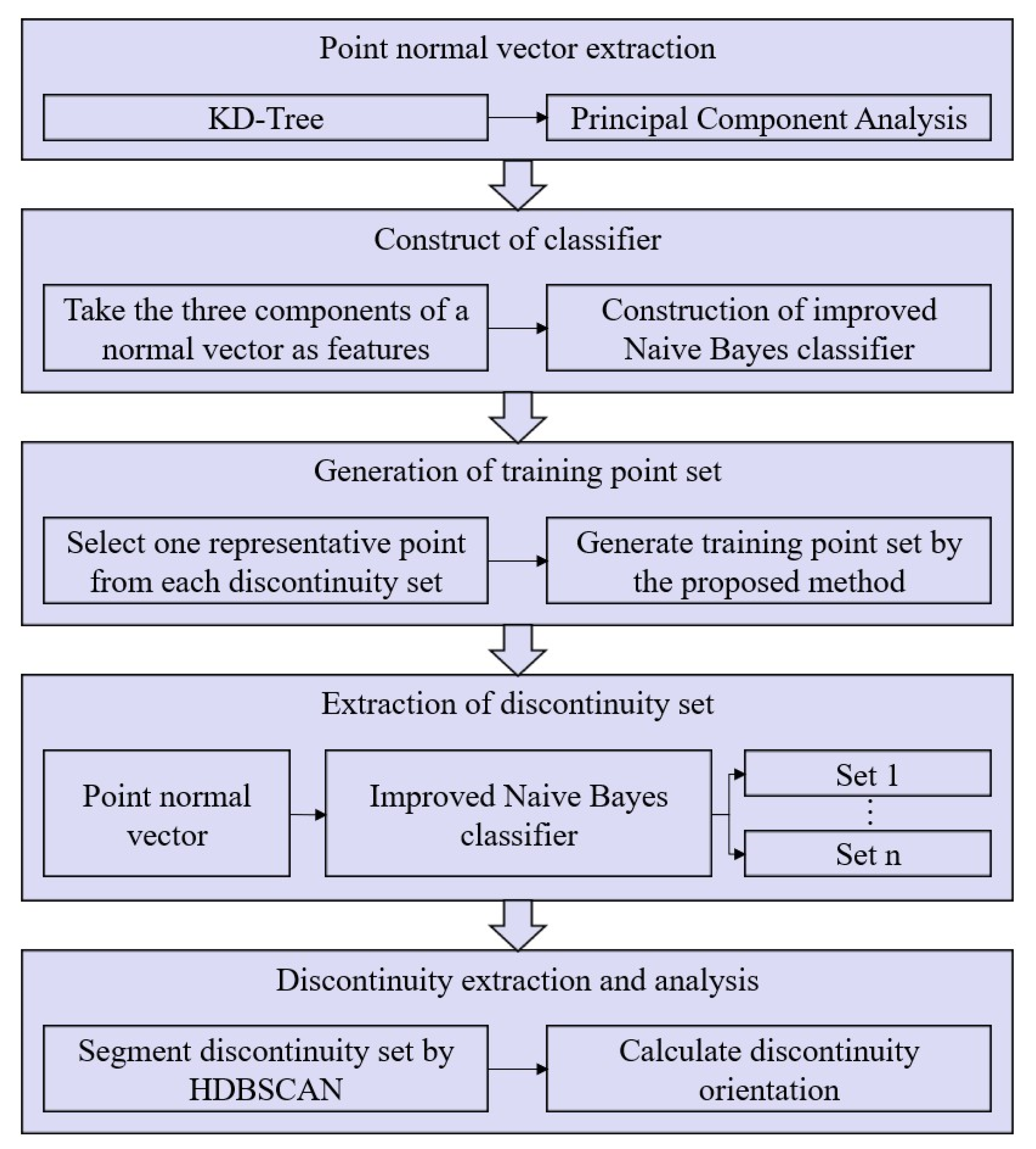
2. Methodology
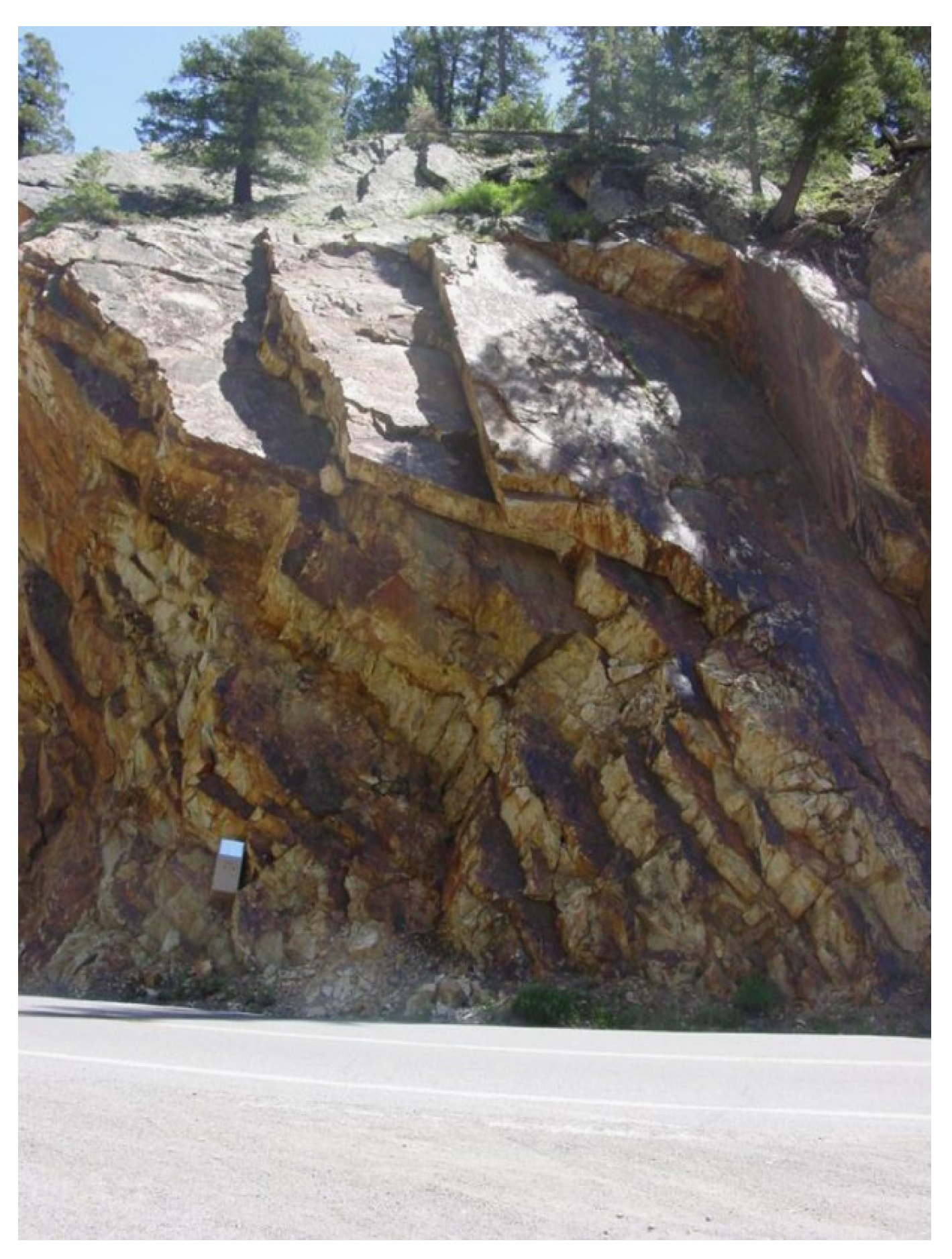
2.1. Case Study A for Validation
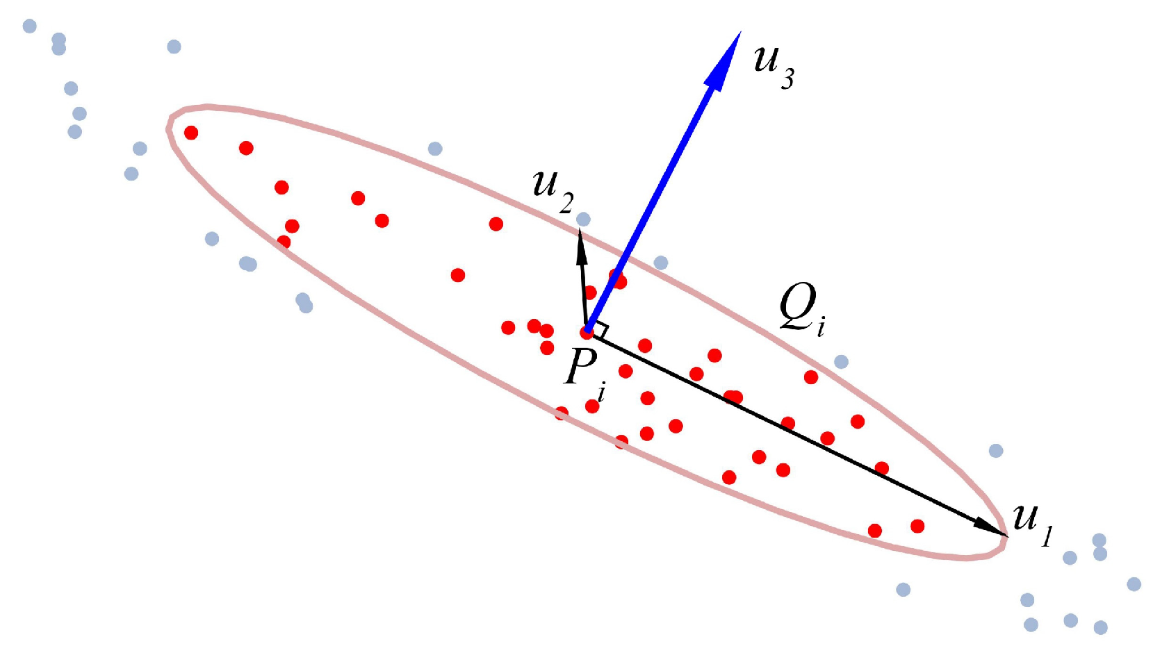
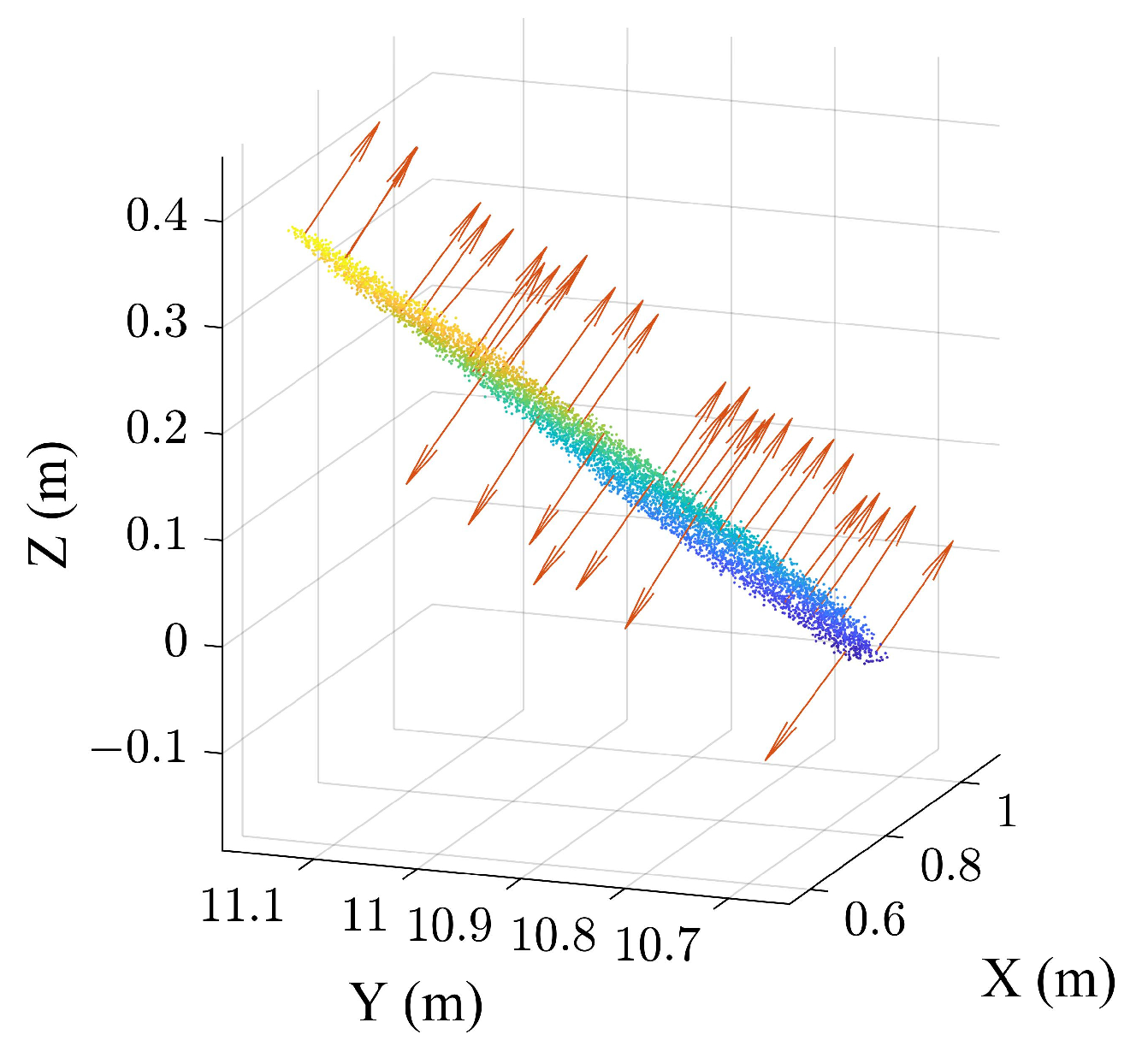
2.2. Extraction of Point Normal Vector
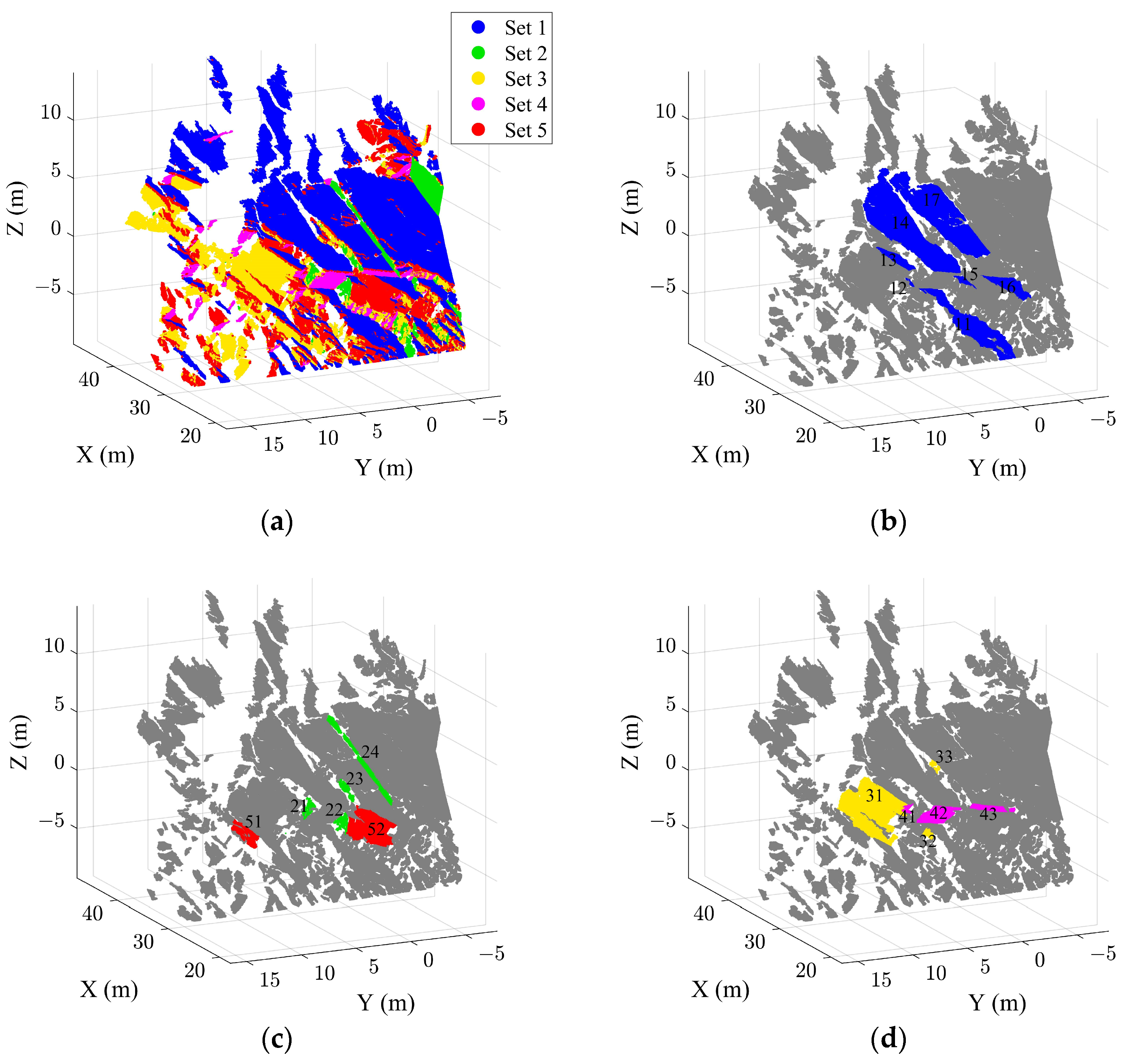
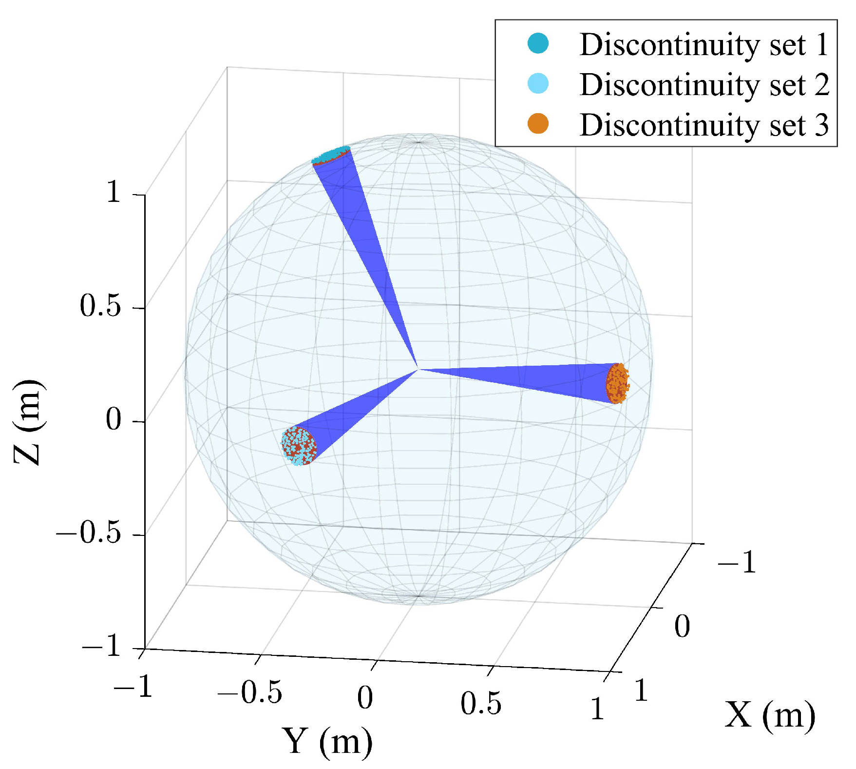
2.3. Extraction of Discontinuity Sets
2.3.1. Construction of the Improved Naive Bayes Classifier
2.3.2. Generation of Training Set
2.3.3. Extraction of Discontinuity Sets Based on the Improved Naive Bayes Classifier
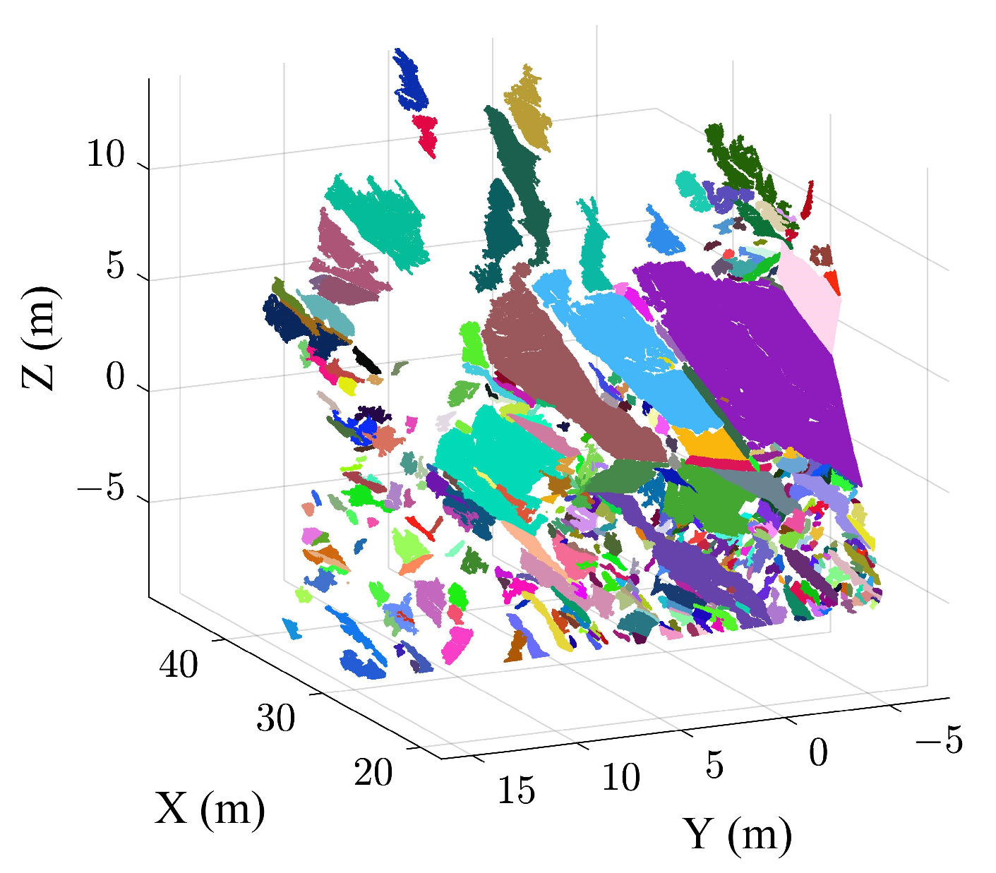
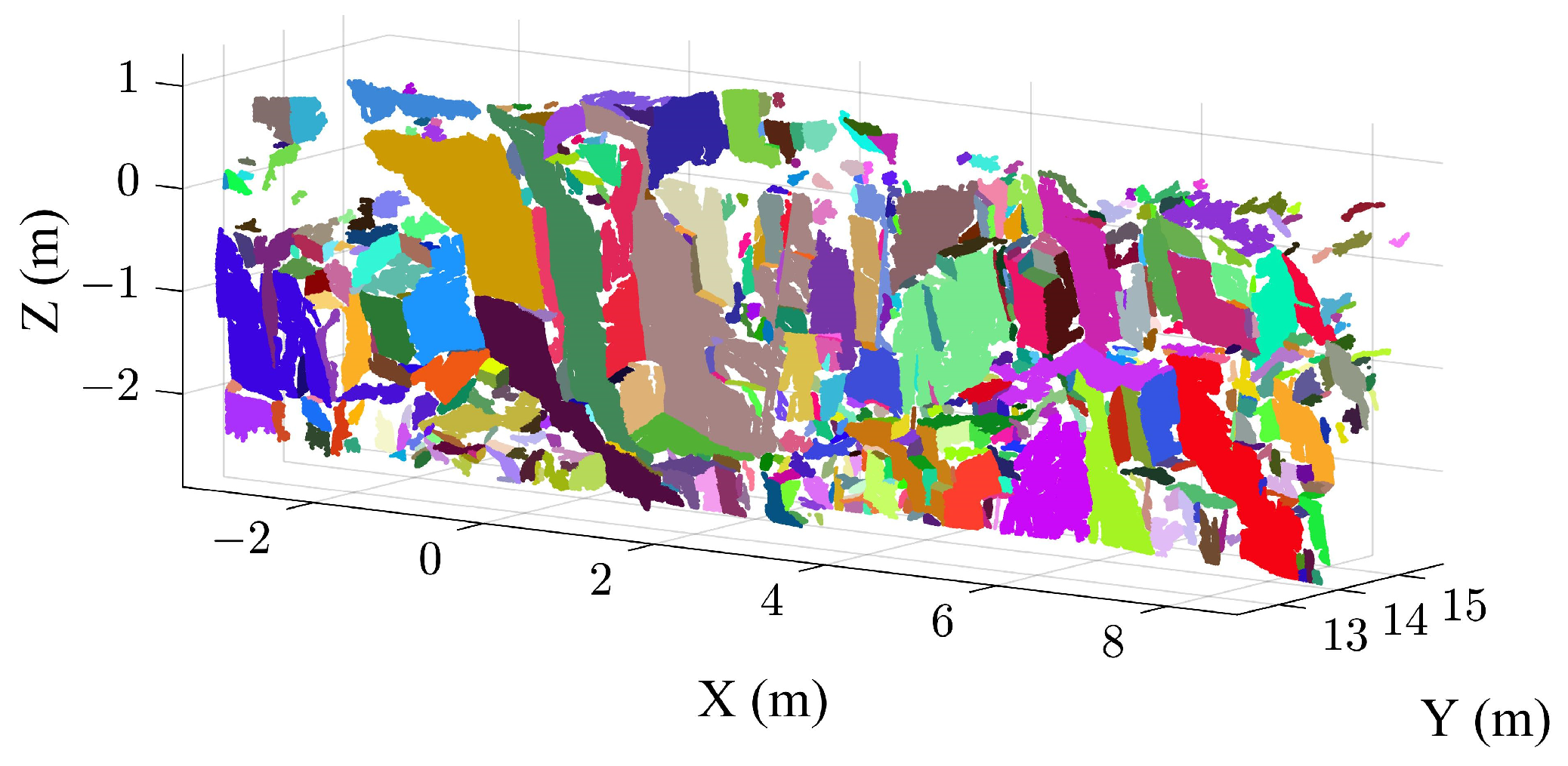
2.4. Extraction of Individual Discontinuity Using the HDBSCAN Algorithm
2.5. Calculation of Rock Discontinuity Parameters
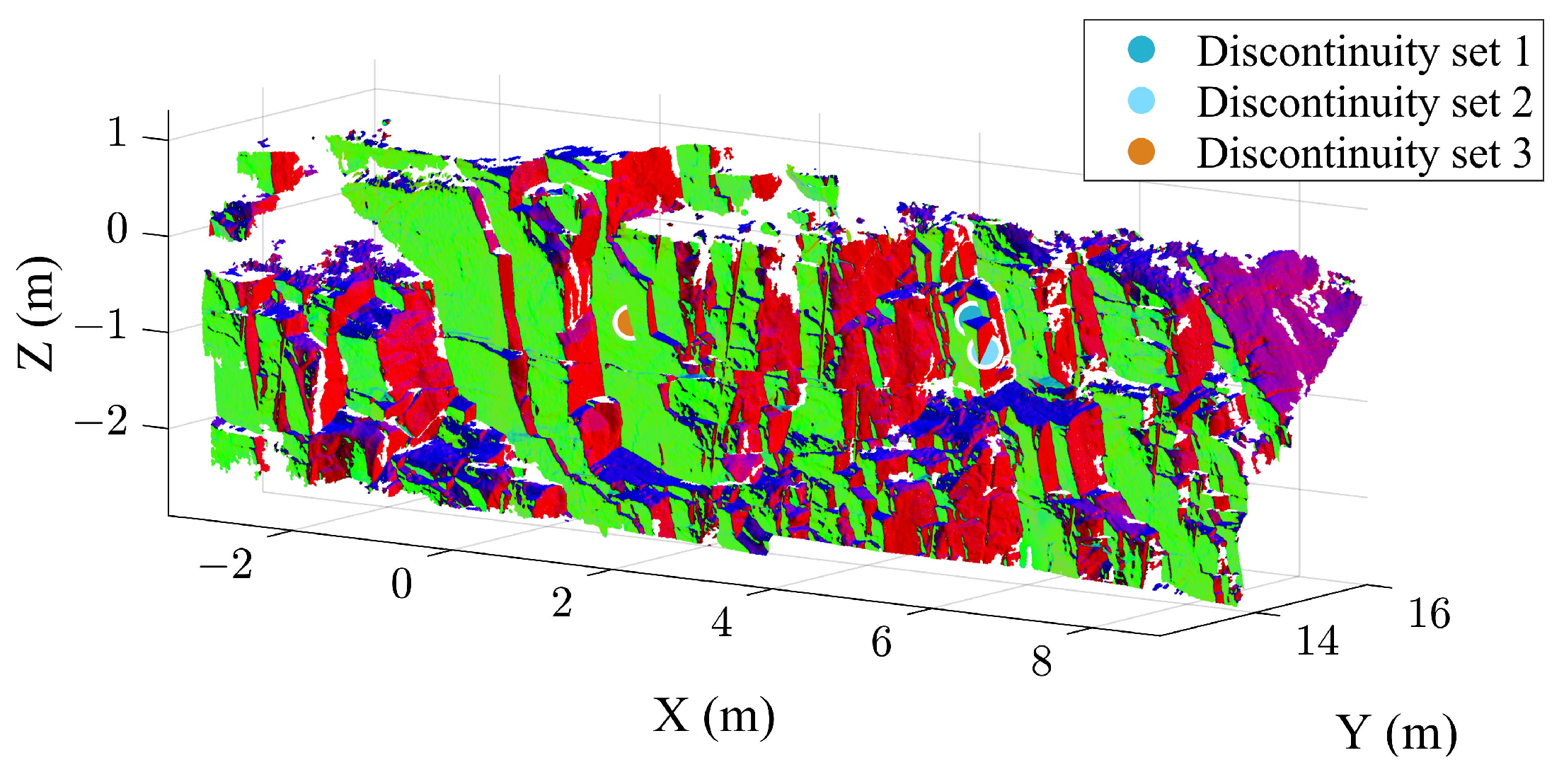
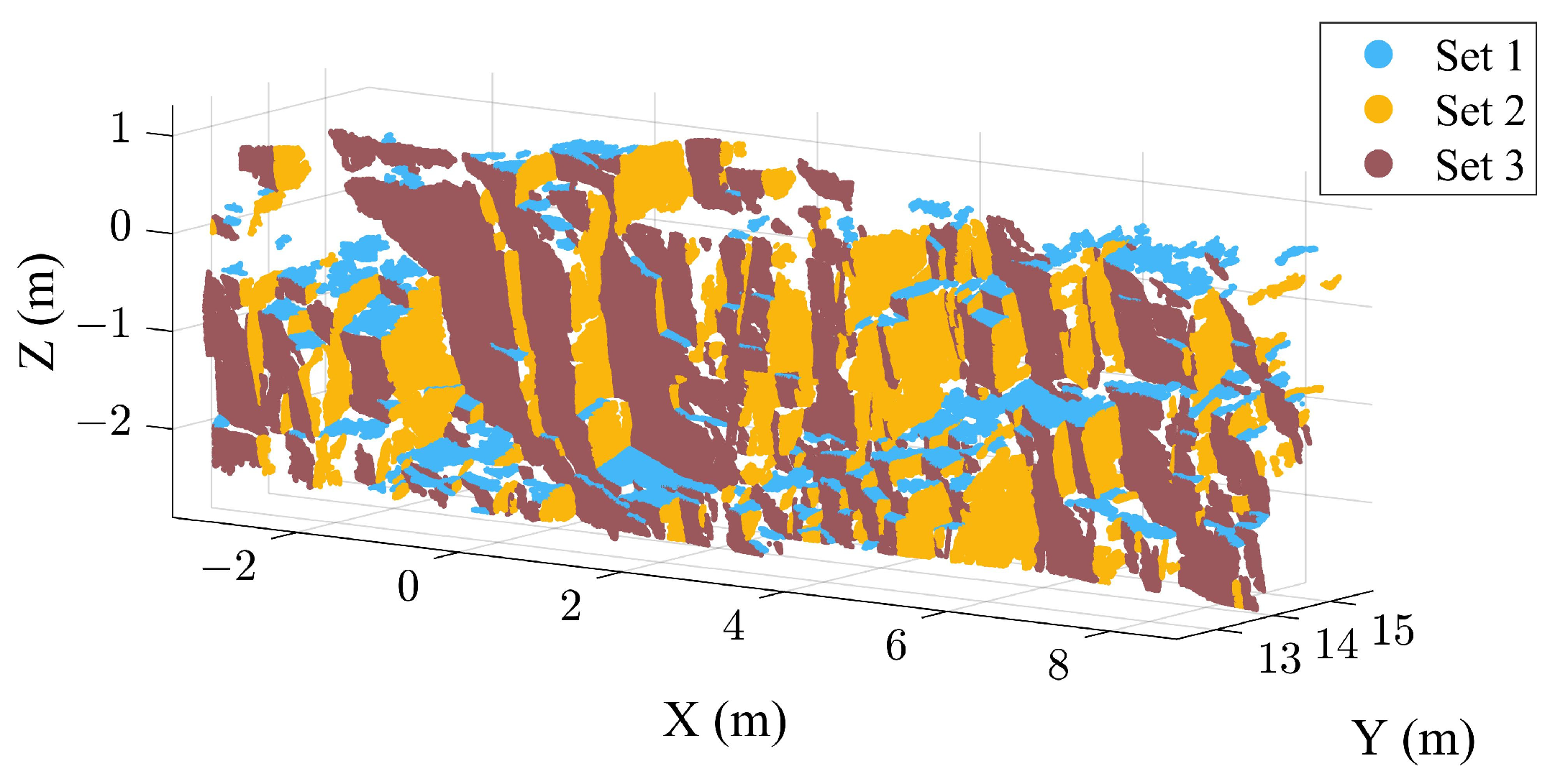
3. Case Study B
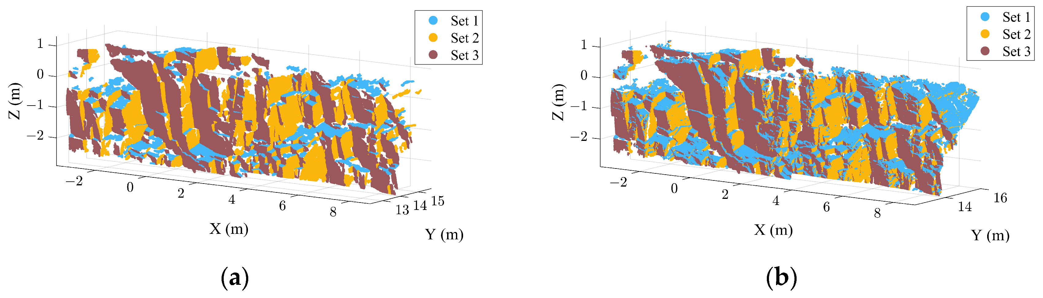
3.1. Extraction Results of the Case B
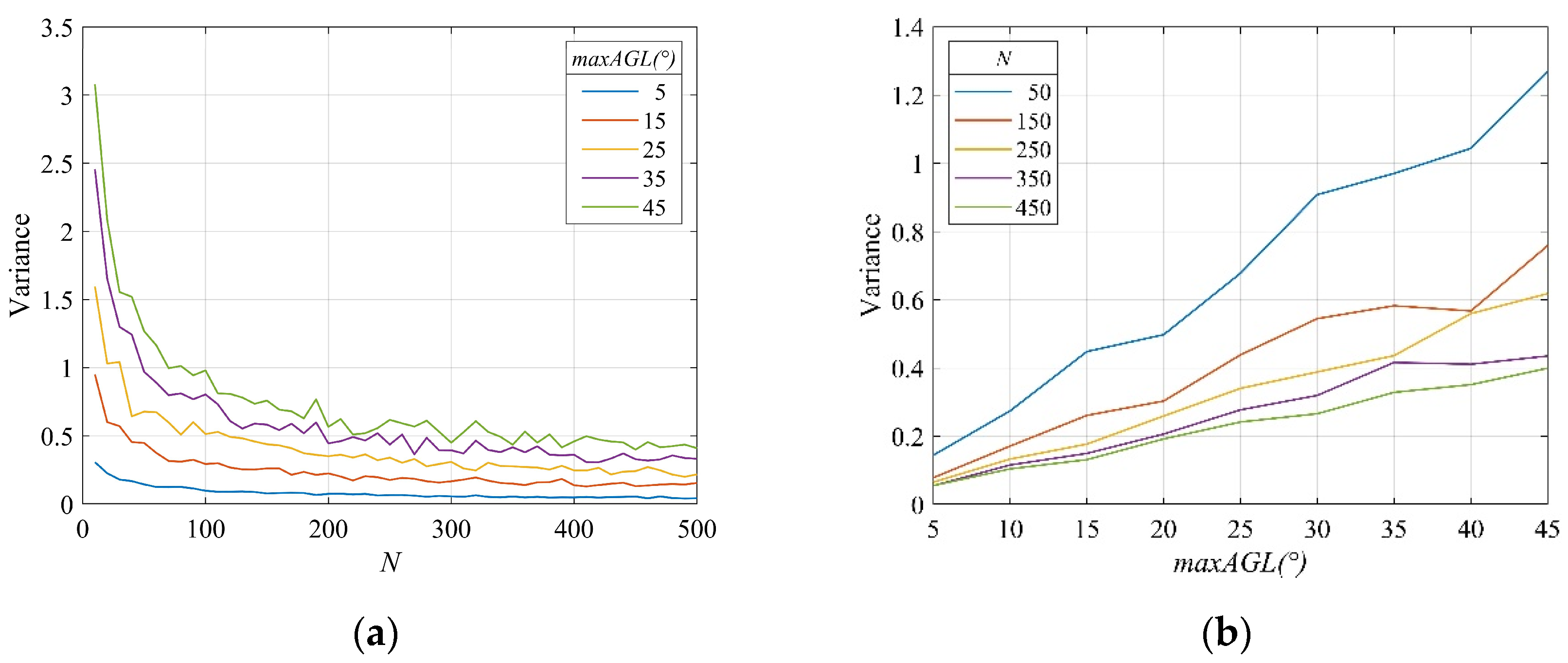
3.2. Maximum Angle maxAGL and Quantity N for Training Sets Generation
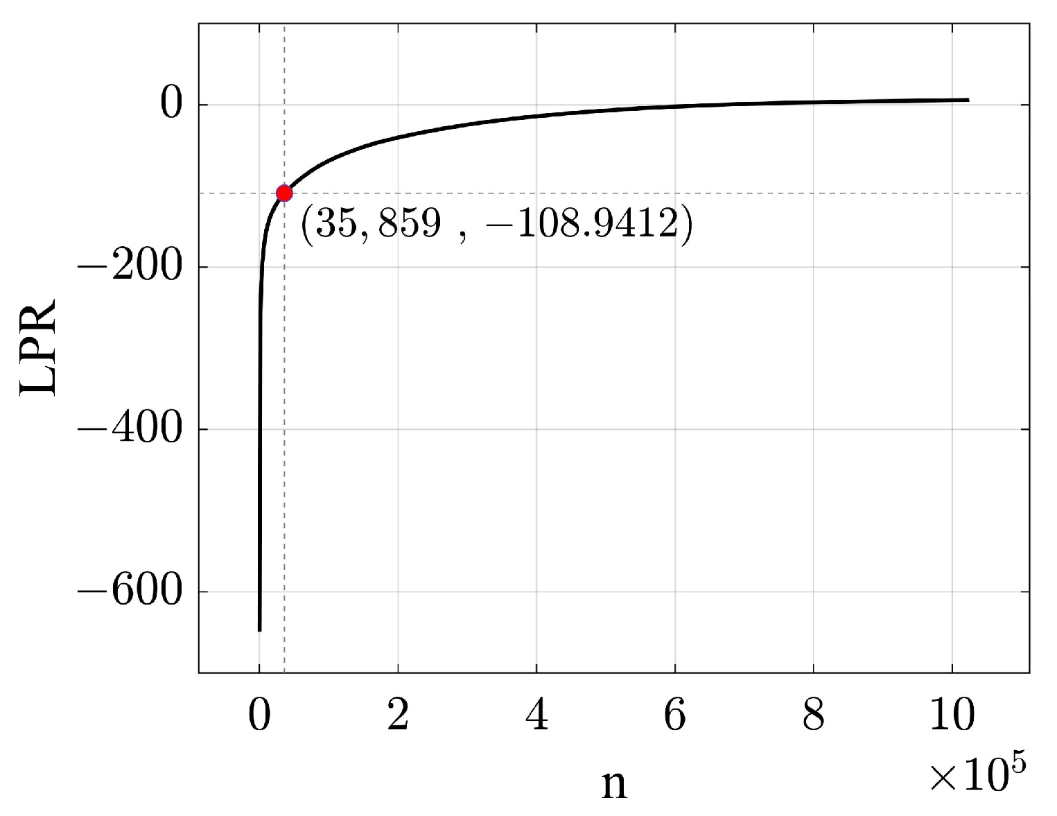
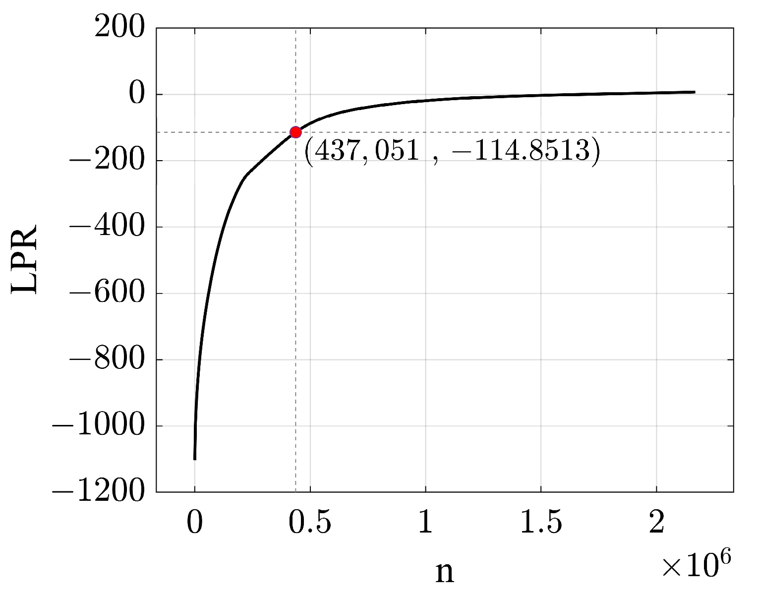
3.3. Minimum Logarithmic Probability minLPR
4. Discussion
5. Conclusions
Author Contributions
Funding
Institutional Review Board Statement
Informed Consent Statement
Data Availability Statement
Acknowledgments
Conflicts of Interest
References
- Slob, S. Automated Rock Mass Characterisation Using 3-D Terrestrial Laser Scanning. Ph.D. Thesis, Delft University of Technology, Delft, The Netherlands, 2010. [Google Scholar]
- Ghosh, A.; Daemen, J.J. Fractal Characteristics of Rock Discontinuities. Eng. Geol. 1993, 34, 1–9. [Google Scholar] [CrossRef]
- Zhang, F.; Damjanac, B.; Maxwell, S. Investigating Hydraulic Fracturing Complexity in Naturally Fractured Rock Masses Using Fully Coupled Multiscale Numerical Modeling. Rock Mech. Rock Eng. 2019, 52, 5137–5160. [Google Scholar] [CrossRef]
- Barton, N.R. Suggested Methods for the Quantitative Description of Discontinuities in Rock Masses. Int. J. Rock Mech. Min. Sci. Geomech. Abstr. 1978, 15, 319–368. [Google Scholar]
- Bieniawski, Z.T. Engineering Rock Mass Classifications: A Complete Manual for Engineers and Geologists in Mining, Civil, and Petroleum Engineering; John Wiley & Sons: Hoboken, NJ, USA, 1989; ISBN 0-471-60172-1. [Google Scholar]
- Sturzenegger, M.; Stead, D. Close-Range Terrestrial Digital Photogrammetry and Terrestrial Laser Scanning for Discontinuity Characterization on Rock Cuts. Eng. Geol. 2009, 106, 163–182. [Google Scholar] [CrossRef]
- Mah, J.; Samson, C.; McKinnon, S.D. 3D Laser Imaging for Joint Orientation Analysis. Int. J. Rock Mech. Min. Sci. 2011, 48, 932–941. [Google Scholar] [CrossRef]
- Gigli, G.; Casagli, N. Semi-Automatic Extraction of Rock Mass Structural Data from High Resolution LIDAR Point Clouds. Int. J. Rock Mech. Min. Sci. 2011, 48, 187–198. [Google Scholar] [CrossRef]
- Kong, D.; Wu, F.; Saroglou, C. Automatic Identification and Characterization of Discontinuities in Rock Masses from 3D Point Clouds. Eng. Geol. 2020, 265, 105442. [Google Scholar] [CrossRef]
- Priest, S.D.; Hudson, J. Discontinuity Spacings in Rock. Int. J. Rock Mech. Min. Sci. Geomech. Abstr. 1976, 13, 135–148. [Google Scholar] [CrossRef]
- Gischig, V.; Amann, F.; Moore, J.; Loew, S.; Eisenbeiss, H.; Stempfhuber, W. Composite Rock Slope Kinematics at the Current Randa Instability, Switzerland, Based on Remote Sensing and Numerical Modeling. Eng. Geol. 2011, 118, 37–53. [Google Scholar] [CrossRef]
- Zhang, P.; Zhao, Q.; Tannant, D.D.; Ji, T.; Zhu, H. 3D Mapping of Discontinuity Traces Using Fusion of Point Cloud and Image Data. Bull. Eng. Geol. Environ. 2019, 78, 2789–2801. [Google Scholar] [CrossRef]
- Lato, M.; Diederichs, M.S.; Hutchinson, D.J.; Harrap, R. Optimization of LiDAR Scanning and Processing for Automated Structural Evaluation of Discontinuities in Rockmasses. Int. J. Rock Mech. Min. Sci. 2009, 46, 194–199. [Google Scholar] [CrossRef]
- Umili, G.; Ferrero, A.; Einstein, H. A New Method for Automatic Discontinuity Traces Sampling on Rock Mass 3D Model. Comput. Geosci. 2013, 51, 182–192. [Google Scholar] [CrossRef]
- Li, X.; Chen, Z.; Chen, J.; Zhu, H. Automatic Characterization of Rock Mass Discontinuities Using 3D Point Clouds. Eng. Geol. 2019, 259, 105131. [Google Scholar] [CrossRef]
- Roncella, R.; Forlani, G. Extraction of Planar Patches from Point Clouds to Retrieve Dip and Dip Direction of Rock Discontinuities. In Proceedings of the ISPRS Workshop Laser Scanning, Enschede, The Netherlands, 12–15 September 2005; pp. 162–167. [Google Scholar]
- Ferrero, A.M.; Forlani, G.; Roncella, R.; Voyat, H. Advanced Geostructural Survey Methods Applied to Rock Mass Characterization. Rock Mech. Rock Eng. 2009, 42, 631–665. [Google Scholar] [CrossRef]
- Chen, J.; Zhu, H.; Li, X. Automatic Extraction of Discontinuity Orientation from Rock Mass Surface 3D Point Cloud. Comput. Geosci. 2016, 95, 18–31. [Google Scholar] [CrossRef]
- Chen, N.; Kemeny, J.; Jiang, Q.; Pan, Z. Automatic Extraction of Blocks from 3D Point Clouds of Fractured Rock. Comput. Geosci. 2017, 109, 149–161. [Google Scholar] [CrossRef]
- Leng, X.; Xiao, J.; Wang, Y. A Multi-Scale Plane-Detection Method Based on the Hough Transform and Region Growing. Photogramm. Rec. 2016, 31, 166–192. [Google Scholar] [CrossRef]
- Yang, S.; Liu, S.; Zhang, N.; Li, G.; Zhang, J. A Fully Automatic-Image-Based Approach to Quantifying the Geological Strength Index of Underground Rock Mass. Int. J. Rock Mech. Min. Sci. 2021, 140, 104585. [Google Scholar] [CrossRef]
- Jaboyedoff, M.; Oppikofer, T.; Abellán, A.; Derron, M.-H.; Loye, A.; Metzger, R.; Pedrazzini, A. Use of LIDAR in Landslide Investigations: A Review. Nat. Hazards 2012, 61, 5–28. [Google Scholar] [CrossRef]
- Gomes, R.K.; de Oliveira, L.P.; Gonzaga Jr, L.; Tognoli, F.M.; Veronez, M.R.; de Souza, M.K. An Algorithm for Automatic Detection and Orientation Estimation of Planar Structures in LiDAR-Scanned Outcrops. Comput. Geosci. 2016, 90, 170–178. [Google Scholar] [CrossRef]
- Wang, X.; Zou, L.; Shen, X.; Ren, Y.; Qin, Y. A Region-Growing Approach for Automatic Outcrop Fracture Extraction from a Three-Dimensional Point Cloud. Comput. Geosci. 2017, 99, 100–106. [Google Scholar] [CrossRef]
- Ge, Y.; Tang, H.; Xia, D.; Wang, L.; Zhao, B.; Teaway, J.W.; Chen, H.; Zhou, T. Automated Measurements of Discontinuity Geometric Properties from a 3D-Point Cloud Based on a Modified Region Growing Algorithm. Eng. Geol. 2018, 242, 44–54. [Google Scholar] [CrossRef]
- Yi, X.; Feng, W.; Wang, D.; Yang, R.; Hu, Y.; Zhou, Y. An Efficient Method for Extracting and Clustering Rock Mass Discontinuities from 3D Point Clouds. Acta Geotech. 2023, 18, 3485–3503. [Google Scholar] [CrossRef]
- Hu, L.; Xiao, J.; Wang, Y. Efficient and Automatic Plane Detection Approach for 3-D Rock Mass Point Clouds. Multimed. Tools Appl. 2020, 79, 839–864. [Google Scholar] [CrossRef]
- Yu, D.; Xiao, J.; Wang, Y. High-Precision Plane Detection Method for Rock-Mass Point Clouds Based on Supervoxel. Sensors 2020, 20, 4209. [Google Scholar] [CrossRef]
- Singh, S.K.; Banerjee, B.P.; Lato, M.J.; Sammut, C.; Raval, S. Automated Rock Mass Discontinuity Set Characterisation Using Amplitude and Phase Decomposition of Point Cloud Data. Int. J. Rock Mech. Min. Sci. 2022, 152, 105072. [Google Scholar] [CrossRef]
- Park, J.; Cho, Y.K. Point Cloud Information Modeling: Deep Learning–Based Automated Information Modeling Framework for Point Cloud Data. J. Constr. Eng. Manag. 2022, 148, 04021191. [Google Scholar] [CrossRef]
- Slob, S.; Hack, R.; Turner, A.K. An Approach to Automate Discontinuity Measurements of Rock Faces Using Laser Scanning Techniques. In Proceedings of the ISRM EUROCK, Madeira, Portugal, 25–28 November 2002; ISRM: London, UK, 2002; p. ISRM-EUROCK-2002-006. [Google Scholar]
- Riquelme, A.J.; Abellán, A.; Tomás, R.; Jaboyedoff, M. A New Approach for Semi-Automatic Rock Mass Joints Recognition from 3D Point Clouds. Comput. Geosci. 2014, 68, 38–52. [Google Scholar] [CrossRef]
- Menegoni, N.; Giordan, D.; Perotti, C.; Tannant, D.D. Detection and Geometric Characterization of Rock Mass Discontinuities Using a 3D High-Resolution Digital Outcrop Model Generated from RPAS Imagery–Ormea Rock Slope, Italy. Eng. Geol. 2019, 252, 145–163. [Google Scholar] [CrossRef]
- Wu, X.; Wang, F.; Wang, M.; Zhang, X.; Wang, Q.; Zhang, S. A New Method for Automatic Extraction and Analysis of Discontinuities Based on TIN on Rock Mass Surfaces. Remote Sens. 2021, 13, 2894. [Google Scholar] [CrossRef]
- Van Knapen, B.; Slob, S. Identification and Characterisation of Rock Mass Discontinuity Sets Using 3D Laser Scanning. Procedia Eng. 2006, 191, 838–845. [Google Scholar]
- Vöge, M.; Lato, M.J.; Diederichs, M.S. Automated Rockmass Discontinuity Mapping from 3-Dimensional Surface Data. Eng. Geol. 2013, 164, 155–162. [Google Scholar] [CrossRef]
- Olariu, M.I.; Ferguson, J.F.; Aiken, C.L.; Xu, X. Outcrop Fracture Characterization Using Terrestrial Laser Scanners: Deep-Water Jackfork Sandstone at Big Rock Quarry, Arkansas. Geosphere 2008, 4, 247–259. [Google Scholar] [CrossRef]
- Li, Y.; Wang, Q.; Chen, J.; Xu, L.; Song, S. K-Means Algorithm Based on Particle Swarm Optimization for the Identification of Rock Discontinuity Sets. Rock Mech. Rock Eng. 2015, 48, 375–385. [Google Scholar] [CrossRef]
- Cui, X.; Yan, E. A Clustering Algorithm Based on Differential Evolution for the Identification of Rock Discontinuity Sets. Int. J. Rock Mech. Min. Sci. 2020, 126, 104181. [Google Scholar] [CrossRef]
- Guo, J.; Liu, S.; Zhang, P.; Wu, L.; Zhou, W.; Yu, Y. Towards Semi-Automatic Rock Mass Discontinuity Orientation and Set Analysis from 3D Point Clouds. Comput. Geosci. 2017, 103, 164–172. [Google Scholar] [CrossRef]
- Xu, W.; Zhang, Y.; Li, X.; Wang, X.; Ma, F.; Zhao, J.; Zhang, Y. Extraction and Statistics of Discontinuity Orientation and Trace Length from Typical Fractured Rock Mass: A Case Study of the Xinchang Underground Research Laboratory Site, China. Eng. Geol. 2020, 269, 105553. [Google Scholar] [CrossRef]
- Chen, J.; Huang, H.; Zhou, M.; Chaiyasarn, K. Towards Semi-Automatic Discontinuity Characterization in Rock Tunnel Faces Using 3D Point Clouds. Eng. Geol. 2021, 291, 106232. [Google Scholar] [CrossRef]
- Ge, Y.; Cao, B.; Tang, H. Rock Discontinuities Identification from 3D Point Clouds Using Artificial Neural Network. Rock Mech. Rock Eng. 2022, 55, 1705–1720. [Google Scholar] [CrossRef]
- Bayes, F.R.S. An Essay towards Solving a Problem in the Doctrine of Chances. Biometrika 1958, 45, 296–315. [Google Scholar] [CrossRef]
- McCallum, A.; Nigam, K. A Comparison of Event Models for Naive Bayes Text Classification. In Proceedings of the AAAI-98 Workshop on Learning for Text Categorization, Madison, WI, USA, 26–27 June 1998; Volume 752, pp. 41–48. [Google Scholar]
- Berchialla, P.; Foltran, F.; Gregori, D. Naïve Bayes Classifiers with Feature Selection to Predict Hospitalization and Complications Due to Objects Swallowing and Ingestion among European Children. Saf. Sci. 2013, 51, 1–5. [Google Scholar] [CrossRef]
- Feng, X.; Li, S.; Yuan, C.; Zeng, P.; Sun, Y. Prediction of Slope Stability Using Naive Bayes Classifier. KSCE J. Civ. Eng. 2018, 22, 941–950. [Google Scholar] [CrossRef]
- Lato, M.; Kemeny, J.; Harrap, R.; Bevan, G. Rock Bench: Establishing a Common Repository and Standards for Assessing Rockmass Characteristics Using LiDAR and Photogrammetry. Comput. Geosci. 2013, 50, 106–114. [Google Scholar] [CrossRef]
- Kemeny, J.; Turner, K.; Norton, B. LIDAR for Rock Mass Characterization: Hardware, Software, Accuracy and Best-Practices. In Laser and Photogrammetric Methods for Rock Face Characterization; ARMA: Golden, CO, USA, 2006; pp. 49–62. [Google Scholar]
- Huang, C.M.; Tseng, Y.-H. Plane Fitting Methods of LIDAR Point Cloud. In Proceedings of the 29th Asian Conference on Remote Sensing 2008, ACRS 2008, Colombo, Sri Lanka, 10–14 November 2008; pp. 1925–1930. [Google Scholar]
- Tsangaratos, P.; Ilia, I. Landslide Susceptibility Mapping Using a Modified Decision Tree Classifier in the Xanthi Perfection, Greece. Landslides 2016, 13, 305–320. [Google Scholar] [CrossRef]
- Campello, R.J.; Moulavi, D.; Sander, J. Density-Based Clustering Based on Hierarchical Density Estimates. In Proceedings of the Pacific-Asia Conference on Knowledge Discovery and Data Mining, Gold Coast, Australia, 14–17 April 2013; Springer: Berlin/Heidelberg, Germany, 2013; pp. 160–172. [Google Scholar]
- Satopaa, V.; Albrecht, J.; Irwin, D.; Raghavan, B. Finding a “Kneedle” in a Haystack: Detecting Knee Points in System Behavior. In Proceedings of the 2011 31st International Conference on Distributed Computing Systems Workshops, Minneapolis, MN, USA, 20–24 June 2011; IEEE: Piscataway, NJ, USA, 2011; pp. 166–171. [Google Scholar]


| Discontinuity ID | Riquelme et al. [32] (°) | Chen et al. [18] (°) | New Method (°) | Riquelme et al. [32] (°) | Chen et al. [18] (°) | ||
|---|---|---|---|---|---|---|---|
| Δ|DD| | Δ|DA| | Δ|DD| | Δ|DA| | ||||
| 11 | 246.24/39.02 | 244.62/38.38 | 246.25/39.03 | 0.01 | 0.01 | 1.63 | 0.65 |
| 12 | 256.86/52.3 | 256.18/52.16 | 247.13/49.76 | 9.73 | 2.54 | 9.05 | 2.4 |
| 13 | 70.26/35.8 | 251.04/36.17 | 250.23/35.79 | 0.03 | 0.01 | 0.81 | 0.38 |
| 14 | 252.68/35.48 | 251.44/33.85 | 252.63/35.47 | 0.05 | 0.01 | 1.19 | 1.62 |
| 15 | 249.74/35.91 | 250.82/36.83 | 249.33/35.55 | 0.41 | 0.36 | 1.49 | 1.28 |
| 16 | 70.47/35.91 | 250.46/35.86 | 250.19/35.71 | 0.28 | 0.2 | 0.27 | 0.15 |
| 17 | 255.12/32.82 | 253.19/33.46 | 254.90/30.87 | 0.22 | 1.95 | 1.71 | 2.59 |
| 21 | 339.47/83.25 | 157.55/83.81 | 339.38/82.79 | 0.09 | 0.46 | 1.83 | 1.02 |
| 22 | 166.33/76.58 | 166.31/78.73 | 166.64/77.31 | 0.31 | 0.73 | 0.33 | 1.42 |
| 23 | 160.2/89.86 | 157.52/86.88 | 159.43/89.14 | 0.77 | 0.72 | 1.91 | 2.26 |
| 24 | 173.55/76.85 | 353.07/77.82 | 173.77/77.83 | 0.22 | 0.98 | 0.7 | 0.01 |
| 31 | 136.59/82.58 | 314.73/80.04 | 135.33/81.71 | 1.26 | 0.87 | 0.6 | 1.67 |
| 32 | 131.23/82.67 | 136.52/89.85 | 137.43/87.91 | 6.2 | 5.24 | 0.91 | 1.94 |
| 33 | 143.91/89.7 | 145.62/89.85 | 323.94/89.89 | 0.03 | 0.19 | 1.68 | 0.04 |
| 41 | 97.55/63.22 | 285.98/59.84 | 99.33/62.05 | 1.78 | 1.17 | 6.65 | 2.21 |
| 42 | 91.07/50.19 | 272.57/47.64 | 272.75/48.46 | 1.68 | 1.73 | 0.18 | 0.82 |
| 43 | 96.64/47.97 | 277.31/49.31 | 96.72/47.79 | 0.08 | 0.18 | 0.59 | 1.52 |
| 51 | 123.42/76.15 | 305.04/77.62 | 122.67/75.92 | 0.75 | 0.23 | 2.37 | 1.7 |
| 52 | 105.75/69.94 | 109.29/76.61 | 106.65/69.93 | 0.9 | 0.01 | 2.64 | 6.68 |
| Maximum deviation | 9.73 | 5.24 | 9.05 | 6.68 | |||
| Average deviation | 1.31 | 0.93 | 1.92 | 1.60 | |||
| Discontinuity Set | Number of Points | Number of Discontinuities | Lato (°) | Proposed Method (°) | Deviation (°) |
|---|---|---|---|---|---|
| 1 | 229,036 | 173 | 194/34 | 194/31 | 0/3 |
| 2 | 1,080,620 | 188 | 29/76 | 35/80 | 6/4 |
| 3 | 450,066 | 149 | 309/90 | 136/86 | 7/4 |
Disclaimer/Publisher’s Note: The statements, opinions and data contained in all publications are solely those of the individual author(s) and contributor(s) and not of MDPI and/or the editor(s). MDPI and/or the editor(s) disclaim responsibility for any injury to people or property resulting from any ideas, methods, instructions or products referred to in the content. |
© 2024 by the authors. Licensee MDPI, Basel, Switzerland. This article is an open access article distributed under the terms and conditions of the Creative Commons Attribution (CC BY) license (https://creativecommons.org/licenses/by/4.0/).
Share and Cite
Lu, G.; Zhu, X.; Cao, B.; Li, Y.; Tao, C.; Yang, Z. A New Approach for Discontinuity Extraction Based on an Improved Naive Bayes Classifier. Appl. Sci. 2024, 14, 2050. https://doi.org/10.3390/app14052050
Lu G, Zhu X, Cao B, Li Y, Tao C, Yang Z. A New Approach for Discontinuity Extraction Based on an Improved Naive Bayes Classifier. Applied Sciences. 2024; 14(5):2050. https://doi.org/10.3390/app14052050
Chicago/Turabian StyleLu, Guangyin, Xudong Zhu, Bei Cao, Yani Li, Chuanyi Tao, and Zicheng Yang. 2024. "A New Approach for Discontinuity Extraction Based on an Improved Naive Bayes Classifier" Applied Sciences 14, no. 5: 2050. https://doi.org/10.3390/app14052050
APA StyleLu, G., Zhu, X., Cao, B., Li, Y., Tao, C., & Yang, Z. (2024). A New Approach for Discontinuity Extraction Based on an Improved Naive Bayes Classifier. Applied Sciences, 14(5), 2050. https://doi.org/10.3390/app14052050