Abstract
Predicting the health index of turbofan engines is critical in reducing downtime and ensuring aircraft safety. This study introduces the elite snake optimizer-back propagation (ESO-BP) model to address the challenges of low accuracy and poor stability in predicting the health index of turbofan engines through neural networks. Firstly, the snake optimizer (SO) was improved into the elite snake optimizer (ESO) through an elite-guided strategy and a reverse learning mechanism. The performance improvement was validated using benchmark functions. Additionally, feature importance was introduced as a feature selection method. Finally, the optimization results of the ESO were employed to set the initial weights and biases of the BP neural network, preventing convergence to local optima. The prediction performance of the ESO-BP model was validated using the C-MAPSS datasets. The ESO-BP model was compared with the CNN, RNN, LSTM, baseline BP, and unimproved SO-BP models. The results demonstrated that the ESO-BP model has a superior accuracy with an impressive R-squared () value of 0.931 and a root mean square error () of 0.060 on the FD001 sub-dataset. Furthermore, the ESO-BP model exhibited lower standard deviations of evaluation metrics on 100 trials. According to the study, ESO-BP demonstrated a greater prediction accuracy and stability when compared to commonly used models such as CNN, RNN, LSTM, and BP.
1. Introduction
Turbofan engines are one of the core components of an aircraft [1]. Predicting the remaining useful life (RUL) of the engine and implementing prognostics and health management (PHM) are critical for formulating a targeted maintenance strategy [2]. The turbofan engine health prediction model helps to reduce the risk of unplanned downtime and maximize the operational lifespan [3].
The prediction model for the RUL of turbofan engines is developed based on either their physical structure model or the degradation trends among various monitoring sensors. There are two types of existing methods for estimating RUL: those based on physical models [4,5] and data-driven approaches [6,7,8,9]. Data-driven methods analyze data and identify complex data relationships, achieving accurate predictions of changes in the turbofan engine’s state [10]. Data-driven predictions for the RUL of turbofan engines are influenced by various factors, including the number of operating cycles, operating parameters, and sensor data.
The back-propagation (BP) neural network, which was proposed by Rumelhart et al. [11] in 1986, is a feed-forward neural network trained with the error back-propagation algorithm. It is currently acknowledged as one of the most extensively employed neural network models, celebrated for its simple principles, high computational speed, and robust regression prediction capabilities [12]. However, BP neural networks frequently experience slow convergence and a tendency to become stuck in local optima due to the random selection of initial weights and thresholds [13]. Currently, there is a surge in the use of neural networks coupled with intelligent optimization algorithms. In 2022, Yu et al. [14] introduced a chaotic krill herd algorithm optimized BP neural network, achieving a 3.65% reduction in prediction error for kidney bean yield. Ji and Ding [12] enhanced BP neural networks by utilizing the improved Sparrow Search Algorithm, resulting in an R2 value of 0.99 for sea surface temperature retrieval. Lai et al. [15] introduced the IA-PSO-BP model, which achieved an R2 value of 0.97 for ground pressure prediction.
In the field of intelligent optimization algorithms, Hashim et al. [16] presented a novel algorithm named SO in 2022. However, this algorithm has persistent drawbacks, such as the random movement of individual positions, which may lead to local optima and poor stability. In 2023, Deng and Liu [17] introduced the snow ablation optimizer (SAO), which incorporates elite sets, demonstrating both rapid convergence and a high convergence accuracy.
This study presents an ESO-BP model for predicting the health of turbofan engines. The goal is to enhance the prediction accuracy and stability of the BP neural network in the context of predicting turbofan engine health. The subsequent sections are organized as follows: Section 2 introduces the elite snake optimizer (ESO). Section 3 elaborates on the proposed model architecture. Section 4 covers the experimental specifics, results, and analysis. Section 5 discusses the findings. Finally, Section 6 concludes the study.
2. Elite Snake Optimizer
Intelligent optimization algorithms, also known as optimization techniques or metaheuristic algorithms, are computational methods designed to iteratively explore solution spaces with the aim of discovering the optimal solution to a problem [18]. These algorithms are often inspired by natural processes or phenomena and strive to efficiently navigate complex and high-dimensional spaces in search of the best possible solution [18].
2.1. Snake Optimizer
The SO draws inspiration from the behavioral traits of snakes, specifically, their fighting, foraging, mating, and reproduction behaviors. The algorithm utilizes a group of snake agents to explore the search space and aims to achieve a global optimum based on the fitness values of individual agents. The algorithm also takes into account environmental factors that influence different snake behaviors, such as temperature and food quantity. The equations for updating the environmental factors are provided below [16].
Here, represents the temperature, signifies the current iteration, denotes the maximum iterations, stands for the food quantity, and is a constant value.
Unlike other algorithms, the SO takes a step further in emulating biological behavior. The SO directs the population individuals through unique positional transitions based on the current iterative phase during each iteration of the algorithm [19]. While there are bio-inspired intelligent optimization algorithms such as the sparrow search algorithm (SSA) [20], beluga whale optimization (BWO) [21], and dung beetle optimizer (DBO) [22], which only mimic the predation paths of organisms in their position updating, the SO improves its perceptual capabilities of the search space by simulating the physiological behaviors of snakes in response to environmental changes. This enhancement accelerates the convergence of SO and improves its precision in achieving convergence [19].
2.2. Elite-Guided Strategy
In intelligent optimization algorithms, elite-guided strategies involve selecting or generating a set of individuals with a higher fitness during the population initialization phase. These individuals subsequently influence the movement of others in the following iterations, enhancing the search efficiency and convergence speed of the swarm [23].
Various intelligent optimization algorithms use different elite-guided strategies. For example, in particle swarm optimization (PSO), each particle updates its velocity and position by considering its individual historical best position and the global best position [24]. In ant colony optimization (ACO), ants release pheromones while searching for a path, and subsequent ants select paths based on the concentration of pheromones [25]. The whale optimization algorithm (WOA) designates the current optimal solution as the leader for the population in each iteration, and the rest adjust their positions based on the leader’s location [26].
Elite-guided strategies aim to direct individuals towards regions with a superior fitness, accelerating the convergence process [27]. However, this may result in premature convergence, trapping the algorithm in local optima [27]. Therefore, designing an appropriate elite-guided strategy is a crucial aspect of research on intelligent optimization algorithms.
During the population initialization stage of ESO, an elite-guided strategy is employed. Elite subsets are selected from both the male and female snake populations, each comprising four individuals. The subsets consist of the top three individuals ranked by the fitness of their current position, along with a new individual calculated as the mean coordinate of all individuals in the current population.
Figure 1 illustrates that Elite 1, Elite 2, and Elite 3 expedite the convergence speed of SO in the search space, since they are the three agents closest to the optimal solution. Elite 4 is the new individual calculated as the mean coordinate of all individuals in the current population, which emphasizes the diversity of the population and helps SO to avoid local optima. Equation (3) is used to calculate Elite 4. This strategy aims to achieve a balance between convergence speed and accuracy, thereby enhancing the global search efficiency of SO.
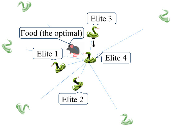
Figure 1.
The elite set of the snake population. The guiders of Elite 1 to 3 are selected by rank of fitness values. The Elite 4 is the mean coordinate of the current snake population.
Here, is the -th dimension value of Elite 4, is the -th dimension value of -th individual, and is the population size.
2.3. Reverse Learning Mechanism
Reverse learning mechanisms are utilized as an enhancement method for intelligent optimization algorithms. The idea is to use symmetric positions within the search space, such as point symmetry, axial symmetry, planar symmetry, or rotational symmetry, to generate reverse populations [28]. The reverse population complements the original solution, maximizes the utilization of the search space, and enhances the algorithm’s ability to overcome local optima [29]. The aim of this method is to improve the algorithm’s global search capability, thereby enhancing the comprehensiveness and effectiveness of the optimization process [29].
During the position update phase of ESO, a reverse learning mechanism is incorporated. This involves assigning opposite values to the positions of the new population within the limits of each dimension, resulting in a mirrored population. The reverse learning mechanism expands the existing population while enhancing the algorithm’s capability to overcome local optima. The calculation for the position of the reverse individual is presented in Equation (4) [28].
In the Equation (4), represents the value of the reverse individual for the -th dimensional coordinate, is the upper boundary of the current search space, is the lower boundary of the current search space, is the value of the original individual for the -th dimensional coordinate.
2.4. Benchmark Test Results
The SO has been enhanced into the elite snake optimizer through the improvements mentioned above. To evaluate the convergence accuracy and stability of the ESO, 30 trials were performed using the 30-dimensional benchmark functions F7, F18, and F30 from the 2017 IEEE Congress on Evolutionary Computation (CEC2017) [30]. Figure 2a–c show the corresponding three-dimensional surface plots with a contour plot underneath.
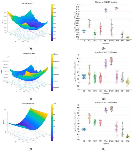
Figure 2.
Comparison of nine algorithms on CEC2017 benchmark functions [30]. (a) Shows the 3D surface plot of 2D function F7 with a contour plot underneath. (b) Shows the results of nine algorithms on 30-D function F7. (c) Shows the 3D surface plot of 2D function F18 with a contour plot underneath. (d) Shows the results of nine algorithms on 30-D function F18. (e) Shows the 3D surface plot of 2D function F30 with a contour plot underneath. (f) Shows the results of nine algorithms on 30-D function F30. The y-axis in (b,d,f) corresponds to the logarithm of the fitness value with base 10.
The CEC2017 test function set is a widely recognized and challenging tool for validating algorithm performance [30]. All functions in the test set are rotated and shifted, which increases the difficulty of algorithmic optimization search. The set consists of 29 test functions, all of which are rotated and shifted to increase the difficulty of the algorithmic optimization search. It is worth noting that the F2 function was officially removed from the original function set due to its instability.
Functions F1 and F3 have a single peak and no local minima, making them suitable for testing the algorithm’s convergence ability. Functions F4–F10 have multiple peaks with local extrema, making them suitable for testing the algorithm’s ability to escape local optima [30]. Functions F11–F20 are hybrids, composed of three or more CEC 2017 baseline functions that have been rotated or shifted. Each subfunction is assigned a weight. Functions F21–F30 are compositions of at least three hybrid functions or CEC 2017 baseline functions that have been rotated or shifted. Each subfunction has an additional bias value and weight, making these combined functions even more challenging to optimize.
The ESO was compared to eight mainstream intelligent optimization algorithms: differential evolution algorithm (DE) [31], PSO, grey wolf optimization (GWO) [32], chicken swarm optimization (CSO) [33], SSA, BWO, DBO, and SO. These algorithms were aimed toward obtaining the global minimum of fitness. The best fitness values of the optimization algorithm were recorded for each trial. The results, as shown in Figure 2b,d,f, demonstrate that ESO has lower means, maximums, and minimums, which indicate a better convergence accuracy. The smaller interquartile range represents the better stability of the ESO algorithm.
3. Model Construction
This study presents an ESO-BP neural network model for predicting the health index of turbofan engines. The model utilizes the optimization results of ESO to initialize the weights and biases of the BP neural network, which prevents it from converging to local optima and improves both prediction accuracy and stability. Figure 3 displays the complete flowchart of ESO-BP.
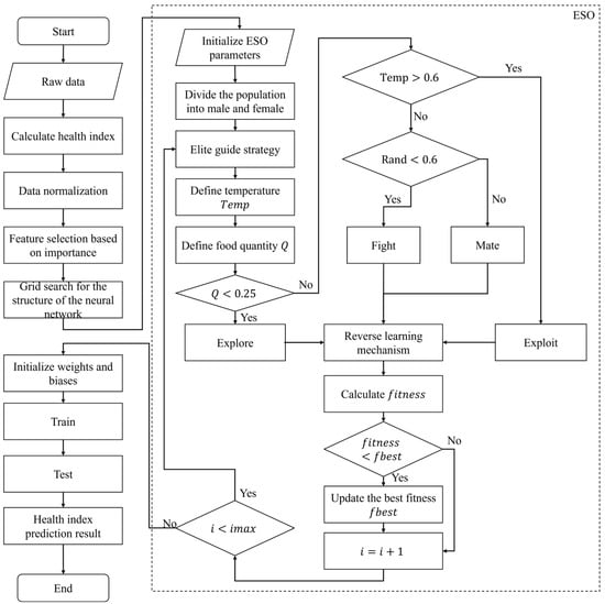
Figure 3.
Flowchart of ESO-BP model. The temperature () and food quantity (Q) is defined in Equations (1) and (2).
3.1. Health Index Degradation
The C-MAPSS dataset defines the remaining useful life of a turbofan engine as the number of remaining operating cycles until a fault occurs. Current research primarily centers on predicting the remaining operating cycles of turbofan engines [6,7,8,9,34,35,36]. However, the remaining operating cycles are influenced by various external and internal factors, resulting in significant errors and a low coefficient of determination between the predicted and actual values. Most prediction modeling studies that focus on the number of remaining operating cycles struggle to capture the degradation of an engine with a substantial RUL greater than 100 cycles.
This study differs from traditional prediction by utilizing a remaining health index () evaluation criterion for turbofan engines. The is constructed based on , and the health of each brand-new engine is initially recorded as ‘1’. The RHI decreases by a certain amount for each operating cycle until the engine stops due to a malfunction, at which point, the becomes ‘0’ [37]. In simpler terms, the is the ratio between the current number of operating cycles remaining for the engine and the maximum number of operating cycles for this engine (), as calculated by Equation (5).
Figure 4 illustrates a visualization that compares the degradation function with existing segmented degradation functions.

Figure 4.
Comparison of RHI and RUL degradation functions.
3.2. Introduction to Datasets
This study uses the publicly available turbofan condition monitoring data from the Commercial Modular Aero-Propulsion System Simulation (C-MAPSS) dataset provided by the National Aeronautics and Space Administration (NASA) to predict the remaining health index of turbofan engines [38]. The C-MAPSS dataset comprises four subsets, each containing various operating and faulty working conditions. Each subset is then divided into a training set and test set, as shown in Table 1.

Table 1.
C-MAPSS dataset information.
The training set records various state parameters of the turbofan engine. These variables include the number of operating cycles and 24 pieces of sensor information. Data are recorded as time series throughout its complete lifespan cycle, from the normal state to the fault state. In contrast, in the test set randomly stops collecting the cycle parameters, meaning that the complete life cycle is not recorded for each engine.
These sensor data include information about the engine’s operating parameters, pressure, and temperature for 24 lots of sensor information, as shown in Table 2, which can be used to train and test fault diagnosis and prediction models. This dataset is widely used in the fields of machine learning and data mining, which provides valuable data support for aero-engine health management.
Table 2.
Feature importance of 4 sub-datasets. The underlined numbers represent the redundant features in the corresponding sub-datasets.
3.3. Feature Selection
In the context of predicting the health of turbofan engines, there are several redundant features. Appropriate feature selection methods can enhance model performance, reduce computational costs, and provide an improved model interpretability.
This study employs a feature selection method based on a random forest. In the random forest model, each decision tree is built by conducting bootstrap sampling from the original dataset [39]. The corresponding out-of-bag data are used to evaluate the prediction error of the -th tree in the random forest. In order to assess the importance of the -th feature, the values of -th feature are randomly permuted and the out-of-bag data prediction error is reevaluated. The importance of the -th feature is determined by calculating the ratio of the average and standard deviation of out-of-bag data errors for all trees in the entire random forest, both before and after disrupting the -th feature. Equation (6) is used to calculate the standard deviation , and Equation (7) is used to calculate the feature importance .
Here, represents the standard deviation of the errors, represents the prediction error after disrupting the -th feature, represents the prediction error before disrupting the -th feature, is the number of trees, and is the importance of the -th feature. In this section, we present the feature importance analysis for FD001, FD002, FD003, and FD004. The results are summarized in Table 2.
Table 2 shows that the FD001 subset has seven redundant features, and the FD003 subset has six redundant features. Redundant features are those with ‘0’ feature importance in Table 2. Upon examining of the raw data, it is evident that the values of these features remain constant during the operating cycles of turbofan engines. To reduce computational costs, these features are excluded from both the comparative and proposed models in this study.
3.4. Data Normalization and Correlation Analysis
When predicting the health index of turbofan engines, there is a significant difference in the order of magnitude between operational parameters and sensor parameters. To train neural networks, each feature needs to be weighted and summed. Without normalizing the original data, some features may carry excessively large weights, while others may have excessively small weights. This can complicate the training of neural networks and affect the predictive performance of the model.
Equation (8) expresses the Min–Max scaling calculation used to normalize both the operational parameters and sensor parameters in the original dataset. The goal is to mitigate the dimensional impact among different features.
Here, represents the minimum of the feature, represents the maximum of the feature, is the original value, and is the normalized value.
The Pearson linear correlation coefficient is the most commonly used linear correlation coefficient [40]. We calculated the Pearson correlation coefficient in order to analyze the correlation between features. Equation (9) shows the calculation of the Pearson correlation coefficient.
Here, is the sample size of the feature, represents the -th sample value of the feature, represents the mean value of the feature, is the -th value of the number of operating cycles, and is the mean value of the number of operating cycles.
For the No. 100 engine in the training set of the FD001, we selected the 15 features with feature importance larger than 0.1 () from its records. We then normalized the original data using Min–Max normalization to obtain the corresponding normalized values. The results of the normalization are presented in Figure 5.
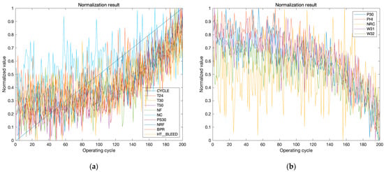
Figure 5.
Normalized features of the No. 100 engine in the training set of FD001. (a) Shows the ten features with an increasing trend and (b) shows the five features with a decreasing trend.
From Figure 5, it seems that 10 out of the 15 features exhibit an increasing trend with the number of engine cycles, while the remaining 5 features show a decreasing trend. Analyzing these changes in degradation can enhance our understanding of the relationship between the engine’s operational state and the features, providing valuable validation for feature selection result. The Pearson correlation coefficients between the number of operating cycles and the other 14 features are presented in Table 3. All the 10 features in Figure 5a show positive Pearson correlation coefficients in Table 3, while the 5 features in Figure 5b present negative values in Table 3. In this way, the values in Table 3 justify the observed result of normalization.
Table 3.
Pearson correlation coefficients between number of operating cycles and all the 25 features of the NO. 100 engine in the training set of FD001. The underlined values present the redundant features.
3.5. BP Neural Network
The BP neural network model’s performance is significantly impacted by the number of hidden layers, number of neurons in the hidden layer, initial weights, and biases. The weights indicate the strength of the connections between neurons, while the biases are additional learnable parameters for neurons that introduce shifts and offsets to the neuron inputs, adjusting the input to the activation function [14].
This study consistently used a single hidden layer for the BP neural networks to control the variable. The number of neurons in the hidden layer was determined using the empirical formula, as shown in Equation (10) [15].
In the equation, represents the number of neurons in the neural network’s hidden layer, represents the number of neurons in the input layer, represents the number of neurons in the output layer, and is a positive integer with a value ranging from 1 to 10.
The optimal value of for finding the number of neurons in the hidden layer was found using grid search. The initial weights and biases of the BP neural network were optimized using ESO. The optimization problem for the weights and biases was formulated in a high-dimensional space, and the fitness function was based on the root mean square error of the BP neural network on training sets [13]. Figure 6 illustrates the optimization process. Equations (11) and (12) are used to calculate the dimensions and fitness values [14].
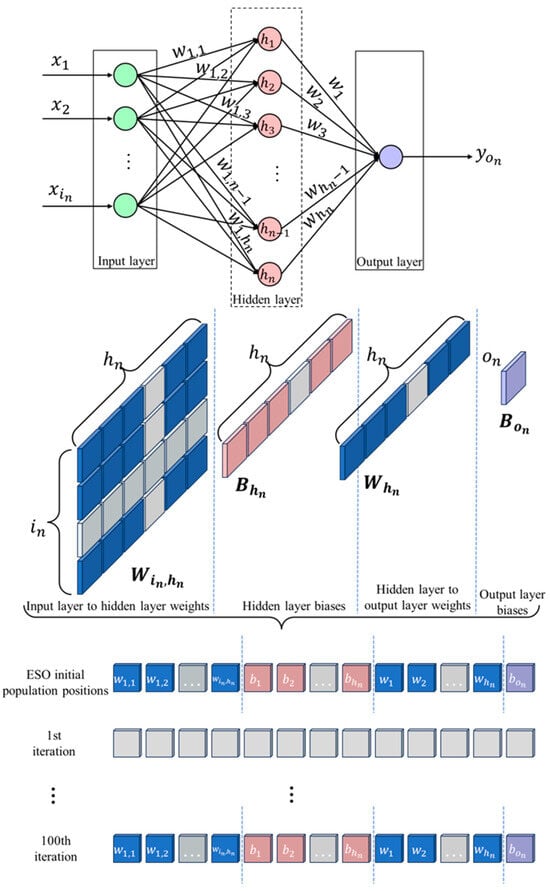
Figure 6.
The ESO optimization process of the BP neural network.
Here, signifies the search space dimension of ESO, is the fitness value of the -th iteration of ESO, indicates the number of samples in the training set, denotes the actual value of the -th sample, and represents the model’s predicted value for the -th sample.
3.6. Parameters of ESO
After determining the number of neurons in the hidden layer using grid search, the dimensionality of the ESO search space is defined based on the model structure. Subsequently, ESO optimizes the initial values of the weights and biases in the BP neural network by establishing the upper and lower bounds of the solution space and specifying the population size [13].
The population size is a crucial parameter in intelligent optimization algorithms. A large population size may increase the computation time required to execute the algorithm, potentially resulting in wasted computational resources. Conversely, a small population size may decrease population diversity, hindering the effective exploration of the solution space and potentially leading to a slower convergence. In addition, an excessively small population may become trapped in local optima, which can cause the global optimum to be missed. Therefore, the parameters of ESO are configured based on the values presented in Table 4.
Table 4.
Parameter values of ESO.
3.7. ESO Optimization Process
The overall framework of the proposed ESO-BP prediction model is illustrated in Figure 7. The implementation of ESO optimization involves the following specific steps:
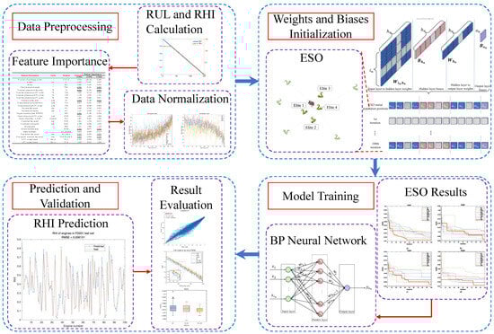
Figure 7.
Framework overview for RHI prediction of turbofan engines.
- 1.
- Employ grid search to determine the optimal number of neurons in the hidden layer and establish the optimal structure for the BP neural network model.
- 2.
- Initialize the parameters for ESO, define the dimensions and value ranges of the search space based on the optimal model structure, and specify the population size, maximum iteration count, and fitness function using Equations (10)–(12).
- 3.
- Randomly generate the initial population, compute the fitness value for each individual, and identify the elite sets for both the male and female populations.
- 4.
- In the early iterations, the populations enter the exploration phase due to the quantity of food being lower than 0.25. In this phase, individuals in both the male and female populations randomly select an elite guider and move to positions near it. The exploration phase is presented in Equation (13) [16].Here, is the -th individual position and is the current iteration count. is the position of a randomly selected elite guider in an elite set. is the fitness of the elite guider. is the fitness of the -th individual. and are the upper and lower bounds of the problem, respectively.
- 5.
- In the later stages of iteration, the populations enter the exploitation phase when the food quantity exceeds 0.25. In this phase, the behavior of the populations is influenced by the temperature. If the temperature is greater than the threshold, both male and female individuals move toward the population’s optimal position (food). If the temperature is lower than the threshold, there is a 40% probability that male and female populations engage in conflict, and a 60% probability that they engage in mating. The snake fight stage is defined in Equations (14) and (15). The snake mating stage is defined in Equations (16) and (17). The calculation for updating the worst individual is defined in Equation (18).In Equations (14)–(18), and are the positions of the -th individual in the male and female populations, and are the positions of the optimal individuals in the male and female populations, and are the fitness values of the optimal individuals in the male and female populations, and are the fitness values of current male or female individuals, and is the food quantity defined in Equation (2) [16].
- 6.
- Generate reverse populations using Equation (4). If there is a new individual with better fitness, the ESO algorithm will replace the original agent with the new individual.
- 7.
- Continuously adjust the position of the snake agent until reaching the maximum iteration count, obtaining the optimal spatial position.
- 8.
- Based on the coordinates of the optimal solution, set the weights from the input layer to the hidden layer, the biases for the hidden layer, the weights from the hidden layer to the output layer, and the biases for the output layer for the BP neural network.
The pseudo-code of ESO is defined as Algorithm 1:
| Algorithm 1 The pseudo-code of ESO |
| Stage 1. Initialization Initialized Problem Setting (d, , , n, T) |
| Generate the ESO population . |
| Calculate the fitness () of each individual of population. |
| Divide the ESO population into two equal groups. Generate the Elite-Guided set. |
| Stage 2. ESO Iteration for Calculate Temp using Equation (1). Calculate Q using Equation (2). if then end if Calculate Elite 4 using Equation (3). Select Elite 1, Elite2, and Elite 3 according to the fitness. if then Perform exploration using Equation (13). else if then Perform exploitation, all individuals move to food. else if then Male population fight with female population using Equations (14) and (15). else Snakes mate using Equations (16) and (17). Update the worst individual using Equation (18). end if end if Generate reverse populations using Equation (4). Calculate fitness of reverse individuals . if Change the best solution to reverse individual. end if end for Return optimal solution. |
4. Simulation Experiments and Result Analysis
4.1. Description to Hyperparameters
To achieve a better forecasting performance, it is essential to systematically optimize the relevant hyperparameters of the models. These hyperparameters include the number of hidden layer nodes, learning rate, and the size of the training batch. To ensure the control of the variables in later comparison experiments among different sub-datasets and deep learning models, we used empirical values of 1 for the number of hidden layers, 1000 for the max iteration epochs, 128 for the batch size, and 0.01 for the initial learning rate of BP neural networks. To achieve a higher accuracy, the number of hidden nodes can be tuned sequentially in the range given by Equation (11), while keeping the other parameters unchanged. Figure 8 presents the grid search result of the number of hidden nodes. According to Figure 8, the number of nodes in the hidden layer of BP neural networks was taken as 13.
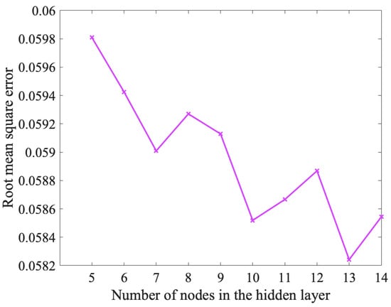
Figure 8.
Grid search for the number of hidden nodes. The search range was determined by Equation (11).
4.2. Model Evaluation Metrics
To evaluate the accuracy of the prediction model proposed in this study, three evaluation metrics were used. The root mean square error was used to measure the difference between the predicted and actual values. This metric indicates the average deviation between predicted and actual values and is commonly used in regression tasks. A smaller RMSE value indicates a greater accuracy, and its unit is the same as that of the original data. The is calculated using Equation (19).
The coefficient of determination, which represents the model’s explanatory power for the dependent variable, has a range of values from 0 to 1. A higher value indicates a better fit of the model to the data. The is calculated using Equation (20).
It is better for the predicted health index of the turbofan engine to be slightly underestimated rather than overestimated [35]. If the predicted health index cannot reach zero before a failure occurs, it poses a serious safety hazard to the aircraft. To address this issue, this study employs a scoring function () proposed by the International Conference on Prognostics and Health Management (PHM08) Data Challenge [38]. The scoring function penalizes situations where the model’s predicted values are larger more severely. The score is calculated by Equations (21) and (22).
From Equation (19) to Equation (22), indicates the predicted value of the -th sample, while denotes its real value and is the total number of samples.
4.3. Optimization Results
To evaluate the optimization ability of various intelligent optimization algorithms on BP neural networks, we optimized the initial weights and biases of the networks using the eight comparison algorithms mentioned above. The population size, number of iterations, and limits of the solution space for all eight algorithms were controlled to be the same as ESO above. The fitness function of the optimization problem was selected as the RMSE of the BP neural network on the training set. The convergence curves of the nine algorithms are depicted in Figure 9.
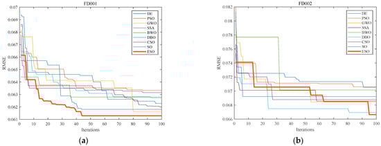
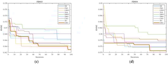
Figure 9.
Convergence curves of nine algorithms optimizing BP neural networks for all four sub-datasets. (a) Convergence curves for FD001; (b) convergence curves forFD002; (c) convergence curves for FD003; and (d) convergence curves for FD004. The x-axis in the figures corresponds to the number of algorithm iterations, while the y-axis represents the root mean square error.
In Figure 9, all nine algorithms improved the accuracy of BP neural networks. However, BWO and SSA performed as the worst and the second worst, respectively, in the simulation test of the benchmark functions F18 and F30. Correspondingly, BWO performed the worst in optimizing the initial weights and biases in FD003 and FD004, while SSA performed the second worst in FD001 and FD003. Furthermore, ESO demonstrated a faster and more precise convergence than SO in all four sub-datasets. The performance indicators in simulation and practice were consistent with each other. These findings lead to three conclusions: 1. Using intelligent optimization to initialize the weights and biases of the BP neural network is an effective method for improving model prediction accuracy; 2. The more suitable the weights and biases found by initialization methods, the more accurate the prediction performed by BP neural networks; and 3. ESO, enhanced by the elite-guided strategy and reverse learning mechanism, has both theoretical and practical performance improvements.
Figure 9 shows the convergence curves of DE, PSO, GWO, SSA, BWO, DBO, CSO, SO, and ESO in optimizing the fitting of BP neural networks to four different sub-datasets. After 100 iterations, ESO achieved a 7.356% reduction in the RMSE of the BP neural network on the FD001 sub-dataset. This result demonstrates that ESO can enhance the prediction accuracy of the BP neural network for the RHI prediction problem in turbofan engines within a relatively small number of iterations. Compared to the other eight mainstream optimization algorithms, ESO converged to smaller fitness values. This indicates that ESO is more suitable for optimizing the BP neural network on turbofan engine RHI prediction.
4.4. Prediction Results
The ESO-BP model was used to predict the health index of engines in subsets FD001, FD002, FD003, and FD004 of C-MAPSS. In FD001, the predicted and actual health indexes of the last operating cycle for all engines in the test set were compared. Figure 10 shows slight errors in the RHI prediction of each engine’s last cycle. This indicates that the proposed method can accurately predict the RHI of turbofan engines. Additionally, four engines were randomly selected from the test set to compare the predicted and actual values of the health degradation curves. Figure 11 shows the fitting ability of the degradation trend for four engines in FD001. The results indicate that ESO-BP demonstrates a high accuracy in multivariate input and univariate output prediction.
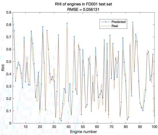
Figure 10.
Comparison of predicted and real RHI of FD001 dataset.
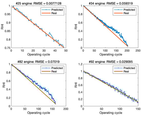
Figure 11.
Comparison of predicted and real degradation curves of four engines in FD001 test set.
4.5. Comparative Experiments
To evaluate the prediction accuracy and stability of ESO-BP, we compared its performance with that of convolutional neural network (CNN), recurrent neural network (RNN), long short-term memory (LSTM), and BP neural networks trained using two different functions. The CNN, RNN, and LSTM models employed in this study used the Adam optimizer [41] for training. BP(SCG) and ESO-BP(SCG) were trained using the scaled conjugate gradient (SCG) backpropagation algorithm [42]. BP(LM) and ESO-BP(LM) were trained using the Levenberg–Marquardt (LM) backpropagation algorithm [43].
Table 5 displays the averages (Avg) and standard deviations (Std) of the evaluation metrics after 100 model training turns. The results indicate that ESO-BP consistently outperformed mainstream models in all the evaluation metrics, proving the effectiveness of the ESO-BP neural network model in predicting the RHI of turbofan engines.
Table 5.
Comparison of different prediction models for 100 trials. The bold number represents the best model.
The results demonstrate that ESO-BP(LM) attained the highest prediction stability, showcasing the smallest standard deviation across all evaluation metrics. This suggests that combining the LM algorithm with improved initial values assists neural networks in avoiding local optima, leading to increased stability. In terms of prediction accuracy, ESO-BP(LM) outperformed in FD001, FD002, and FD004, showcasing a superior predictive capability across various operational conditions. The R2 and RMSE of ESO-BP(SCG) on FD003 were slightly better than those of ESO-BP(LM), indicating that predicting the RHI of turbofan engines under multi-fault conditions poses a particular challenge. ESO improved the performance of BP neural networks with both SCG and LM, indicating that using ESO to initialize BP neural networks is a beneficial approach. The BP neural networks in the following study were trained with the LM algorithm for a better performance, according to the results in Table 5.
To illustrate the deviation between the predicted and real RHI values for each operating cycle of all test set engines in FD001, the real RHI value serves as the horizontal axis, and the predicted RHI value serves as the vertical axis in Figure 12. The deviation between predicted and real values for the different models is shown in Figure 12. The majority of the scatter points from the four models align closely with the reference line. This figure illustrates that the ESO-BP(LM) neural network model exhibits fewer anomalous scatter points and achieves the best prediction results. Figure 13 shows that the predicted RHI degradation curves of the turbofan engines using the proposed method are closer to the real degradation curves compared to other models.
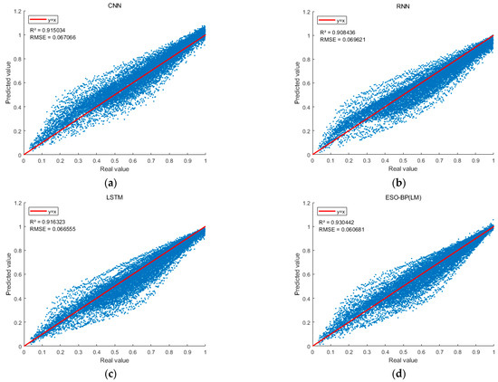
Figure 12.
Scatter of predicted RHI and real RHI values: (a) is the CNN model; (b) is the RNN model; (c) is the LSTM model; and (d) is the ESO-BP model. The blue scatter plot represents the comparison between the predicted RHI values and the real RHI values. The y-axis denotes the predicted RHI values, while the x-axis presents to the real RHI values of FD001.
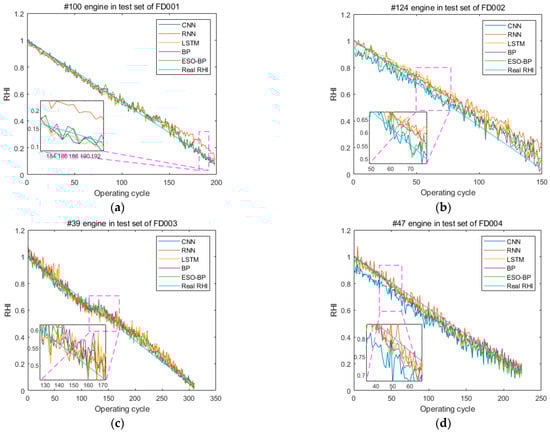
Figure 13.
Comparing the RHI degradation prediction results of different models on four engines: (a) is the No. 100 engine in the test set of FD001; (b) is the No. 124 engine in the test set of FD002; (c) is the No. 39 engine in the test set of FD003; and (d) is the No. 47 engine in the test set of FD004.
4.6. Ablation Experiment
An ablation experiment was conducted to assess the impact of each enhancement approach on the BP model. The experiment compared the baseline BP(LM) with SO-BP(LM) and ESO-BP(LM). Table 6 presents the average evaluation metrics of 100 trials for BP(LM), SO-BP(LM), and ESO-BP(LM).
Table 6.
Averages of evaluation metrics for the ablation experiment. The bold number represents the best model.
The evaluation metrics derived from 100 trials demonstrate that SO optimized BP neural networks on the FD001, FD002, and FD003 sub-datasets of the C-MAPSS. ESO further enhanced the optimization effect and showed improvement on the FD004 subset, where SO-BP performed poorly. In order to visualize the improvements of SO and ESO on BP neural networks, Figure 14 shows the RMSEs of BP(LM), SO-BP(LM), and ESO-BP(LM).
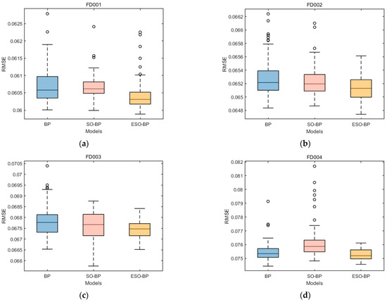
Figure 14.
Boxplots RMSE for BP, SO-BP, and ESO-BP over 100 trials: (a) is the RMSE on FD001; (b) is the RMSE on FD002; (c) is the RMSE on FD003; and (d) is the RMSE on FD004. The box represents the interquartile range, which is the middle 50% of the data. The bottom and top edges of the box correspond to the first quartile and third quartile, respectively. The line inside the box represents the median or the second quartile, which is the middle value of the dataset. The height of the box is the interquartile range. The circles represent the outliers. The y-axis denotes the RMSE values, while the x-axis presents different models.
5. Discussion
The objective of training a neural network is to fine-tune weights and biases to find a parameter set that aligns the predicted values with the actual values as closely as possible [44]. Typically, this process involves finding the global optimal solution, which requires determining the combination of parameters that minimizes the loss function across the entire parameter space. The exceptional prediction performance of the ESO-BP model is attributed to three primary factors: optimizing the initial weights and biases through ESO, employing the RHI metric for turbofan engine degradation, and selecting LM as the training function for BP models.
- 1.
- Initializing neural network weights was demonstrated to accelerate convergence, prevent entrapment in local optima, simplify network architecture, identify feature importance, and improve prediction performance [45]. In this study, adjustments to the initial weights and biases were applied before training to improve the convergence accuracy and stability of the BP neural networks. ESO exhibited a superior convergence compared to SO in benchmark functions. Similarly, in the ablation experiment, ESO-BP outperformed SO-BP. This suggests that providing better initial weights and biases results in higher accuracy and stability in BP neural networks. ESO determined the initial weights and biases that minimized the RMSE after its iteration process, preventing the BP neural network from easily becoming stuck in local optima and experiencing stability issues due to random parameter selection.
- 2.
- In contrast to RUL prediction, Jiang et al. [46] also developed a health index prediction model for turbofan engines in 2023. According to their study, the average accuracy of 10 trials for hybrid methods was significantly lower than that of single methods. Several methods were combined to create multiple new models, including empirical mode decomposition (EMD), variational mode decomposition (VMD), scale-adaptive attention mechanism (SAA), dynamic step size-based fruit fly optimization algorithm (DSSFOA), bidirectional long short-term memory network (BiLSTM), support vector regression (SVR), and LSTM. The average accuracies of the FD002 sub-dataset are compared in Table 7.
Table 7. Comparison of RMSE for hybrid methods [46] and ESO-BP model.
- 3.
- The Levenberg–Marquardt algorithm is particularly effective in training BP neural networks for regression problems [47]. The LM algorithm provides numerical solutions for nonlinear minimization. It combines the strengths of the Gauss–Newton algorithm and the gradient descent method by dynamically adjusting parameters during execution to address the limitations of both methods. When the gradient drops rapidly, the LM algorithm behaves more like the Gauss–Newton algorithm. Otherwise, it behaves more like gradient descent [43].
6. Conclusions
This study improved the convergence performance of an existing optimization algorithm through an elite-guided strategy and a reverse learning mechanism. Simulation experiments were conducted using three benchmark test functions to compare the elite snake optimizer (ESO) with eight mainstream intelligent optimization algorithms. The results indicated that ESO exhibited a higher convergence accuracy and improved stability. Furthermore, ESO was used to initialize the weights and biases of the BP neural network, resulting in the creation of the ESO-BP model. The ESO-BP model was compared with traditional CNN, RNN, LSTM, and a baseline BP neural network in terms of prediction accuracy and stability using the C-MAPSS dataset. The findings showed that the ESO-BP model enhanced the prediction accuracy and stability of BP across all the sub-datasets of C-MAPSS. In conclusion, the ESO-BP model has theoretical significance in improving intelligent optimization algorithms and practical value in predicting the health index of turbofan engines.
In the future, intelligent optimization algorithms can be employed to initialize the parameters for other neural networks and applied across various domains in machine learning. The primary concern is the unacceptable time cost required for intelligent optimization algorithms to search for the global optimum in high-dimensional spaces, attributed to the large number of weights and biases. Accordingly, we will develop effective pruning methods to eliminate specific dimensions of the connection weights, reducing time costs and streamlining the networks. This is a promising research direction.
Author Contributions
Conceptualization, X.Z. and W.D.; methodology, X.Z. and W.D.; software, N.X.; validation, N.X., X.Z. and W.D.; formal analysis, N.X.; investigation, J.W.; resources, G.Z.; data curation, N.X. and W.D.; writing—original draft preparation, X.Z. and N.X.; writing—review and editing, X.Z. and G.Z.; visualization, N.X.; supervision, X.Z. and G.Z.; project administration, X.Z.; funding acquisition, X.Z. All authors have read and agreed to the published version of the manuscript.
Funding
Yunnan Philosophy and Social Sciences Planning Pedagogy Project (AC21012), Humanities and Social Sciences Research Project of Yunnan Provincial Institute and Provincial School Education Cooperation (SYSX202008), the Special Project of “Research on Informatization of Higher Education” of China Society of Higher Education in 2020 (2020XXHYB17).
Institutional Review Board Statement
Not applicable.
Informed Consent Statement
Not applicable.
Data Availability Statement
The data presented in this study are openly available in NASA Prognostics Data Repository at 10.1109/PHM.2008.4711414, accessed on 20 September 2023, reference number [38].
Conflicts of Interest
The authors declare no conflicts of interest.
References
- Zhou, H.; Farsi, M.; Harrison, A.; Parlikad, A.K.; Brintrup, A. Civil aircraft engine operation life resilient monitoring via usage trajectory mapping on the reliability contour. Reliab. Eng. Syst. Saf. 2023, 230, 108878. [Google Scholar] [CrossRef]
- Kordestani, M.; Saif, M.; Orchard, M.E.; Razavi-Far, R.; Khorasani, K. Failure prognosis and applications—A survey of recent literature. IEEE Trans. Reliab. 2019, 70, 728–748. [Google Scholar] [CrossRef]
- Zio, E. Prognostics and health management (PHM): Where are we and where do we (need to) go in theory and practice. Reliab. Eng. Syst. Saf. 2022, 218, 108119. [Google Scholar] [CrossRef]
- Najera-Flores, D.A.; Hu, Z.; Chadha, M.; Todd, M.D. A physics-constrained Bayesian neural network for battery remaining useful life prediction. Appl. Math. Modell. 2023, 122, 42–59. [Google Scholar] [CrossRef]
- Li, X.; Shao, H.; Jiang, H.; Xiang, J. Modified Gaussian convolutional deep belief network and infrared thermal imaging for intelligent fault diagnosis of rotor-bearing system under time-varying speeds. Struct. Health Monit. 2022, 21, 339–353. [Google Scholar]
- Muneer, A.; Taib, S.M.; Naseer, S.; Ali, R.F.; Aziz, I.A. Data-driven deep learning-based attention mechanism for remaining useful life prediction: Case study application to turbofan engine analysis. Electronics 2021, 10, 2453. [Google Scholar] [CrossRef]
- Ren, L.; Qin, H.; Xie, Z.; Li, B.; Xu, K. Aero-engine remaining useful life estimation based on multi-head networks. IEEE Trans. Instrum. Meas. 2022, 71, 3505810. [Google Scholar] [CrossRef]
- Chen, X.; Zeng, M. Convolution-graph attention network with sensor embeddings for remaining useful life prediction of turbofan engines. IEEE Sens. J. 2023, 23, 15786–15794. [Google Scholar] [CrossRef]
- Li, J.; Jia, Y.; Niu, M.; Zhu, W.; Meng, F. Remaining useful life prediction of turbofan engines using CNN-LSTM-SAM approach. IEEE Sens. J. 2023, 23, 10241–10251. [Google Scholar] [CrossRef]
- Li, W.; Zhang, L.-C.; Wu, C.-H.; Wang, Y.; Cui, Z.-X.; Niu, C. A data-driven approach to RUL prediction of tools. Adv. Manuf. 2024, 12, 6–18. [Google Scholar] [CrossRef]
- Rumelhart, D.E.; Hinton, G.E.; Williams, R.J. Learning representations by back-propagating errors. Nature 1986, 323, 533–536. [Google Scholar] [CrossRef]
- Ji, C.; Ding, H. Optimizing back-propagation neural network to retrieve sea surface temperature based on improved sparrow search algorithm. Remote Sens. 2023, 15, 5722. [Google Scholar] [CrossRef]
- Lv, D.; Liu, G.; Ou, J.; Wang, S.; Gao, M. Prediction of GPS satellite clock offset based on an improved particle swarm algorithm optimized BP neural network. Remote Sens. 2022, 14, 2407. [Google Scholar] [CrossRef]
- Yu, L.; Xie, L.; Liu, C.; Yu, S.; Guo, Y.; Yang, K. Optimization of BP neural network model by chaotic krill herd algorithm. Alex. Eng. J. 2022, 61, 9769–9777. [Google Scholar] [CrossRef]
- Lai, X.; Tu, Y.; Yan, B.; Wu, L.; Liu, X. A method for predicting ground pressure in meihuajing coal mine based on improved BP neural network by immune algorithm-particle swarm optimization. Processes 2024, 12, 147. [Google Scholar] [CrossRef]
- Hashim, F.A.; Hussien, A.G. Snake optimizer: A novel meta-heuristic optimization algorithm. Knowl.-Based Syst. 2022, 242, 108320. [Google Scholar] [CrossRef]
- Deng, L.; Liu, S. Snow ablation optimizer: A novel metaheuristic technique for numerical optimization and engineering design. Expert Syst. Appl. 2023, 225, 120069. [Google Scholar] [CrossRef]
- Rahman, M.A.; Sokkalingam, R.; Othman, M.; Biswas, K.; Abdullah, L.; Abdul Kadir, E. Nature-inspired metaheuristic techniques for combinatorial optimization problems: Overview and recent advances. Mathematics 2021, 9, 2633. [Google Scholar] [CrossRef]
- Li, H.; Xu, G.; Chen, B.; Huang, S.; Xia, Y.; Chai, S. Dual-mutation mechanism-driven snake optimizer for scheduling multiple budget constrained workflows in the cloud. Appl. Soft Comput. 2023, 149, 110966. [Google Scholar] [CrossRef]
- Xue, J.; Shen, B. A novel swarm intelligence optimization approach: Sparrow search algorithm. Syst. Sci. Control Eng. 2020, 8, 22–34. [Google Scholar] [CrossRef]
- Zhong, C.; Li, G.; Meng, Z. Beluga whale optimization: A novel nature-inspired metaheuristic algorithm. Knowl.-Based Syst. 2022, 251, 109215. [Google Scholar] [CrossRef]
- Xue, J.; Shen, B. Dung beetle optimizer: A new meta-heuristic algorithm for global optimization. J. Supercomput. 2023, 79, 7305–7336. [Google Scholar] [CrossRef]
- Abduljabbar, D.A.; Hashim, S.Z.M.; Sallehuddin, R. Nature-inspired optimization algorithms for community detection in complex networks: A review and future trends. Telecommun. Syst. 2020, 74, 225–252. [Google Scholar] [CrossRef]
- Miao, K.; Mao, X.; Li, C. Individualism of particles in particle swarm optimization. Appl. Soft Comput. 2019, 83, 105619. [Google Scholar] [CrossRef]
- Talbi, E.-G. Machine learning into metaheuristics: A survey and taxonomy. ACM Comput. Surv. 2021, 54, 129. [Google Scholar] [CrossRef]
- Mirjalili, S.; Lewis, A. The whale optimization algorithm. Adv. Eng. Softw. 2016, 95, 51–67. [Google Scholar] [CrossRef]
- Cai, Y.; Wu, D.; Liu, S.; Fu, S.; Liu, P. Enhancing differential evolution on continuous optimization problems by detecting promising leaders. IEEE Access 2020, 8, 226557–226578. [Google Scholar] [CrossRef]
- Yu, F.; Guan, J.; Wu, H.; Chen, Y.; Xia, X. Lens imaging opposition-based learning for differential evolution with cauchy perturbation. Appl. Soft Comput. 2024, 152, 111211. [Google Scholar] [CrossRef]
- Sahoo, S.K.; Saha, A.K.; Nama, S.; Masdari, M. An improved moth flame optimization algorithm based on modified dynamic opposite learning strategy. Artif. Intell. Rev. 2023, 56, 2811–2869. [Google Scholar] [CrossRef]
- Wu, G.; Mallipeddi, R.; Suganthan, P. Problem Definitions and Evaluation Criteria for the CEC 2017 Competition and Special Session on Constrained Single Objective Real-Parameter Optimization; Technical Report; Nanyang Technological University: Singapore, 2016; pp. 1–18. [Google Scholar]
- Storn, R.; Price, K. Differential evolution–a simple and efficient heuristic for global optimization over continuous spaces. J. Global Optim. 1997, 11, 341–359. [Google Scholar] [CrossRef]
- Mirjalili, S.; Mirjalili, S.M.; Lewis, A. Grey wolf optimizer. Adv. Eng. Softw. 2014, 69, 46–61. [Google Scholar] [CrossRef]
- Meng, X.; Liu, Y.; Gao, X.; Zhang, H. A new bio-inspired algorithm: Chicken swarm optimization. In Proceedings of the Advances in Swarm Intelligence: 5th International Conference, ICSI 2014, Hefei, China, 17–20 October 2014; Part I. pp. 86–94. [Google Scholar]
- Alomari, Y.; Ando, M.; Baptista, M.L. Advancing aircraft engine RUL predictions: An interpretable integrated approach of feature engineering and aggregated feature importance. Sci. Rep. 2023, 13, 13466. [Google Scholar] [CrossRef] [PubMed]
- Hu, K.; Cheng, Y.; Wu, J.; Zhu, H.; Shao, X. Deep bidirectional recurrent neural networks ensemble for remaining useful life prediction of aircraft engine. IEEE Trans. Cybern. 2023, 53, 2531–2543. [Google Scholar] [CrossRef] [PubMed]
- Hou, M.; Pi, D.; Li, B. Similarity-based deep learning approach for remaining useful life prediction. Measurement 2020, 159, 107788. [Google Scholar] [CrossRef]
- Wang, C.; Zhu, Z.; Lu, N.; Cheng, Y.; Jiang, B. A data-driven degradation prognostic strategy for aero-engine under various operational conditions. Neurocomputing 2021, 462, 195–207. [Google Scholar] [CrossRef]
- Saxena, A.; Goebel, K.; Simon, D.; Eklund, N. Damage propagation modeling for aircraft engine run-to-failure simulation. In Proceedings of the 2008 International Conference on Prognostics and Health Management, Denver, CO, USA, 6–9 October 2008; pp. 1–9. [Google Scholar]
- Sun, X.; Chai, J. Random forest feature selection for partial label learning. Neurocomputing 2023, 561, 126870. [Google Scholar] [CrossRef]
- Qin, L.; Yang, G.; Sun, Q. Maximum correlation Pearson correlation coefficient deconvolution and its application in fault diagnosis of rolling bearings. Measurement 2022, 205, 112162. [Google Scholar] [CrossRef]
- Reyad, M.; Sarhan, A.M.; Arafa, M. A modified Adam algorithm for deep neural network optimization. Neural Comput. Appl. 2023, 35, 17095–17112. [Google Scholar] [CrossRef]
- Andrei, N. Scaled conjugate gradient algorithms for unconstrained optimization. Comput. Optim. Appl. 2007, 38, 401–416. [Google Scholar] [CrossRef]
- Ariizumi, S.; Yamakawa, Y.; Yamashita, N. Convergence properties of Levenberg–Marquardt methods with generalized regularization terms. Appl. Math. Comput. 2024, 463, 128365. [Google Scholar] [CrossRef]
- Zhang, J.; Hu, J.; Liu, J. Neural network with multiple connection weights. Pattern Recognit. 2020, 107, 107481. [Google Scholar] [CrossRef]
- Narkhede, M.V.; Bartakke, P.P.; Sutaone, M.S. A review on weight initialization strategies for neural networks. Artif. Intell. Rev. 2022, 55, 291–322. [Google Scholar] [CrossRef]
- Jiang, W.; Xu, Y.; Chen, Z.; Zhang, N.; Xue, X.; Liu, J.; Zhou, J. A feature-level degradation measurement method for composite health index construction and trend prediction modeling. Measurement 2023, 206, 112324. [Google Scholar] [CrossRef]
- Smith, J.S.; Wu, B.; Wilamowski, B.M. Neural network training with Levenberg–Marquardt and adaptable weight compression. IEEE Trans. Neural Networks Learn. Syst. 2018, 30, 580–587. [Google Scholar] [CrossRef]
Disclaimer/Publisher’s Note: The statements, opinions and data contained in all publications are solely those of the individual author(s) and contributor(s) and not of MDPI and/or the editor(s). MDPI and/or the editor(s) disclaim responsibility for any injury to people or property resulting from any ideas, methods, instructions or products referred to in the content. |
© 2024 by the authors. Licensee MDPI, Basel, Switzerland. This article is an open access article distributed under the terms and conditions of the Creative Commons Attribution (CC BY) license (https://creativecommons.org/licenses/by/4.0/).