A Robust Distributed Algorithm for Solving the Economic Dispatch Problem with the Penetration of Renewables and Battery Systems

Abstract

In the field of energy networks, for their effective functioning, it is necessary to distribute the required load between all online generating units in a proper way to cover the demand. The load schedule is obtained by solving the so-called Economic Dispatch Problem (EDP). The EDP can be solved in many ways, resulting in a power distribution plan between online generating units in the network so that the resulting price per unit of energy is minimal. This article focuses on designing a distributed gradient algorithm for solving EDP, supplemented by models of renewable sources, Battery Energy Storage System (BESS), variable fuel prices, and consideration of multiple uncertainties at once. Specifically, these are: time-variable transport delays, noisy gradient calculation, line losses, and drop-off packet representations. The algorithm can thus be denoted as robust, which can work even in unfavorable conditions commonly found in real applications. The capabilities of the presented algorithm will be demonstrated and evaluated on six examples.

1. Motivation

Over the years, significant modifications in the composition of power networks have emerged, and the concept of Smart Grid has been introduced more frequently. This follows the fact that renewable sources and battery systems are increasingly penetrating the current energy grids. They contribute to fast dynamic changes in the grid that need to be considered. Hence, this article addresses such issues of energy networks, especially the EDP. It describes a novel distributed gradient algorithm for solving the EDP.

1.1. Energy Transition towards Dispersed Generation

Nowadays, the energy sector faces several challenges related to various domains covering the whole value chain of electricity delivery, such as energy generation, transmission, and distribution, as well as consumption and dispersed generation. Dispersed generation is the decentralized electricity production using small-scale, diverse energy sources located closer to the point of consumption, promoting grid resilience and sustainability. As a consequence of the implementation of European and worldwide climate strategies (e.g., EU Green Deal, Paris Agreement), the energy sector is progressing through extreme energy transitions, which bring a significant increase in electricity demand (e.g., due to the electrification of mobility) on one side and the strong decarbonization of electricity generation on the other side, for instance. This results in the massive installation of dispersed generation resources (mainly renewables) to the demand side. According to European Network of Transmission System Operators for Electricity (ENTSO-E) Ten-Year Network Development Plan (TYNDP) development scenarios [1], the volume of dispersed generation will significantly increase as depicted in Figure 1. The last three bars on the right side visualize actual global ambitions.

The electricity volume provided by conventional generating units connected to transmission power systems will be continuously shifted to distribution power systems, where dispersed generation is located. According to TYNDP development scenarios, renewable energy generating units (i.e., photovoltaic, wind) will constitute the majority of generating elements. Unfortunately, these renewable generating units are mostly uncontrollable, as shown in some analyses from countries with a highly dispersed generation penetration. For example, Great Britain has reached a high penetration of dispersed generation units [2], representing approximately 35% of the generation mix, as depicted in Figure 2.

The controllable generating units embrace only 41% of overall dispersed generation, while uncontrollable ones represent 59%. This phenomenon drives a significant increase in operational uncertainty at a distribution system level, which implies a notable escalation of volatile power flow exchanges among various parts of distribution power systems. A sufficient operational flexibility volume is required by Distribution System Operators (DSOs) to manage volatile power efficiently flows to maintain reliable and secure distribution system operation, preventing congestion or power quality issues. From a DSO perspective, various stakeholders, operational processes, and tools provide the required operational flexibility, where effective management of technology asset groups (e.g., microgrids, energy communities) located at the demand side represents one possibility discussed in this article.

1.2. Specification of Scope

The electricity value chain has been strongly decoupled in past decades to liberalize and unwrap energy markets (e.g., Winter Package). The electricity value chain can be split into several technology domains such as (i) generation, (ii) transmission, (iii) distribution, and demand side, including (iv) dispersed generation and (v) consumption, as depicted in Figure 3.

In these technology domains, various stakeholders with different business purposes are present. For example, the transmission and distribution domains are operated by transmission system operators and DSOs, respectively. In this paper, the emphasis is put on the demand side, which embraces dispersed generation and consumption connected to a distribution power system. On the demand side, technology asset groups can be considered, which represent real-world entities such as microgrids, energy communities, or virtual power plants. Technology asset groups include a variety of production, consumption, or storage technologies whose coordinated operation enables flexibility for the provision of business services to various stakeholders. For example, the owner of the technology asset group can optimize its operational costs, and the flexibility can be provided to an aggregator for energy market purposes or can be open to DSO for triggering an explicit demand response service to maintain grid reliability and security.

1.3. Technology Asset Groups

The main focus of the paper is on the technology asset groups, which include various technologies with electricity consumption needs, production potential or storage capability (Note, only the electricity part of the energy vector is considered) located in a bounded area (e.g., municipality, selected part of a distribution grid) [3,4,5,6,7]. These assets are connected to distribution grids and are capable of coordinated operation or can work independently. An energy community is a typical case where individual technologies can be operated individually according to user needs or managed according to a selected community operational strategy. Such operational arrangements can be considered coordinated decentralized power systems exchanging information among particular assets to ensure system stability and reliability. This decentralized approach is suitable for heterogeneous environments with various stakeholders and offers resilience and economic savings compared to centralized systems [3,8,9]. Such information flows are drafted in Figure 3 by blue lines among individual assets and create the information topology of the considered network, which defines the communication scheme among individual agents operating a given asset.

The presented work is divided into several parts: Section 2 focuses on analyses and a literature review of the state of the art. Section 3 brings the mathematical formulation of the problem and its boundaries. Next, Section 4 is devoted to the algorithm design, including the construction of models for renewable sources and battery systems. Apart from that, all uncertainties are incorporated into the algorithm. Six simulation examples will be introduced in Section 5. This is followed by Section 6, which deals with Future works and other possible improvements. All outcomes and results are concluded in Section 7.

2. State of the Art

The energy network falls into the section of critical infrastructure. The entire grid has many levels of control and management, according to the technological domain (e.g., transmission grid, distribution grid, demand side) [10,11,12]. Complex optimization tasks, including Unit Commitment and Economic Dispatch (ED), are solved during the operational planning of system elements. The complexity of discrete optimization related to Unit Commitment (i.e., curse of dimensionality) prevents its real-time solution. Therefore, these complex optimization tasks (Unit Commitment complemented by ED) are usually solved in advance [11,12]. Short-term operational planning is solved on the day-ahead time horizon in the case of distribution grids. This task uses statistical methods and models to estimate and forecast this value for a given time frame [13]. The Unit Commitment problem optimizes an activation or deactivation of selected controllable assets (e.g., generators) [14]. On the other hand, the EDP is continuously solved in real-time to manage system disturbances and system state deviations from the expectation when unit commitment has been calculated. The EDP defines operational set points for committed controllable assets (e.g., generators, energy storage) according to the energy needs (i.e., balance) of the energy system, considered optimization constraints and selected control policy. Minimizing operational costs of technology asset groups is often the primary goal [15,16,17].

There are several ways to solve EDP. Article [18] presents a review of methods that were used around 1990. These are mainly centralized solution methods, which include, for example, the Lambda-iteration method or genetic programming [19,20]. Other applicable methods are based on particle swarm optimization or evolutionary programming [21,22,23]. Over the years, efforts have been made to replace these methods with decentralized methods. The inclination towards decentralized methods is mainly thanks to the progress of multi-agent systems theory and technological progress [10,24].

Many consensus-based algorithms are used for a distributed way of solving [8,9,25]. Furthermore, there is also an effort to incorporate renewable sources, mainly from replacing conventional sources to reduce emissions [26,27]. These goals also lead to advancing the technical possibilities of renewable power plants. This development led to the need to manage them across the entire energy network [28]. In order to make greater use of energy from renewable sources, they are often extended by BESS [29,30,31]. BESSs can provide stored energy to the grid but also take it from the grid [30,32]. Due to the growing number of electric cars, the energy network needs to account for them [33]. The next step is the integration of charging stations [34]. This fact leads to the need to ensure stability and cover the required load in the case of networks that consist of different generators, renewables, and BESS.

It is also essential that the distributed methods are applicable even for a large number of considered agents [35]. Paper [36] demonstrates the suitability of distributed algorithms even for many agents, specifically for thousands of generators. Electricity prices change during the day, so it is necessary to adapt to them [37,38]. Mostly, the price is set using an auction-based system, which can be on a different time horizon in Europe; it is usually a 15-min trading interval [39,40]. In order to build such power plants, which will have the lowest possible costs, it is necessary to consider changes in energy prices as well as other costs associated with the operation of generators and the entire energy network. It can sometimes be advantageous for BESS to buy energy at lower prices, then sell it and feed it back into the grid once the price rises.

None of the previously described works represented uncertainties or time delays in the communication network. In realistic cases, however, the communication network is never ideal [41]. The impact of such time delays in communication are described for distributed EDP solution methods in [42,43]. Other problems can be dynamic changes in network topology [44,45] or noisy data transfer between agents [46]. The system representation must also include these communication or data reception uncertainties.

Among the significant topics addressed in 2023 can be selected, for example, the issue of Privacy-Preserving for a distributed EDP solution [47]. Alternatively, it is possible to meet with the effort to reduce the communication complexity of the distributed method of solving using the Dynamic Event-Triggered Algorithm for EDP [48].

This article aims to extend the algorithm proposed in Article [8] with the representation of renewable resources, BESS, variable fuel prices and add more uncertainty at once. In this work, several uncertainties will be considered at the same time, such as time-variable traffic delay, representation of drop-off packets (corrupted or lost data), noisy gradient calculation, and line losses and their treatment. Partial results and extensions by the authors can be found in [49,50,51]. The goal is to provide a robust decentralized algorithm that remains stable even in such cases.

3. Problem Formulation

This paper introduces the distributed optimization method for solving EDP for the technological asset group, where control policy focuses on minimizing operation costs from the owner’s perspective. The main task of EDP is to minimize the total operational costs. At the same time, the overall consumption and limitation of individual technological assets (e.g., generators (generally, controllable units such as generators, controllable loads, etc.)) are considered [8,43,52,53]. The objective function can be formulated as:

$$\begin{array}{c}\hfill \underset{P_i}{min}\sum _{i=1}^N{C}_i\left(P_i\right),\end{array}$$

(1)

where N represents the number of technological assets, $P_i$ is the active power injection related to the i-th asset and $C_i$ denotes the cost function of the i-th asset. Each agent in N, i.e., technological assets, is part of the considered network graph denoted as $\mathcal{G}$. The graph $\mathcal{G}$ indicates the overall shape of the network topology, and on its basis, the communication matrix is constructed later in Section 4.4.

In the next step, the objective function (1) can be detailed to include considered assets such as conventional generating units (i.e., generators), renewable generating units, battery systems, and power grid connection [32,54]. In a distributed optimization approach, each term of an objective function is optimized by an individual agent, which interacts with other ones to achieve optimal system-wide consensus. Consequently, the agents representing these generating resources have their cost functions, which may differ from each other.

The distributed formulation of the objective function minimizing operational costs across all network agents can be expressed as [10,26,30,55,56]:

$$\begin{array}{c}\hfill \min [\underset{\mathrm{Conventional}}{\underbrace{\sum _{i=1}^{N_c}{C}_{c_i}\left(P_{c_i}\right)}}+\underset{\mathrm{Renewables}}{\underbrace{\sum _{i=1}^{N_s}{C}_{s_i}\left(P_{s_i}\right)+\sum _{i=1}^{N_w}{C}_{w_i}\left(P_{w_i}\right)}}+\underset{\mathrm{Energy}\mathrm{storage}}{\underbrace{\sum _{i=1}^{N_b}{C}_{b_i}\left(P_{b_i}\right)}}+\underset{\mathrm{Grid}}{\underbrace{C_g\left(P_g\right)}}],\end{array}$$

(2)

where variable $N_c$ stands for conventional generating assets (microturbines, diesel generators), $N_s$ for photovoltaic plants, $N_w$ for wind power plants, and $N_b$ for battery systems within the network. Additionally, $P_{c_i},P_{s_i},P_{w_i}$, and $P_{b_i}$ represent the power output of generators by type and index i. These types include conventional, solar, wind, and battery systems. Furthermore, $C_{c_i},C_{s_i},C_{w_i}$, and $C_{b_i}$ denote price functions for generators of the respective type and index i. Variable $C_g$ denotes the price function of energy provided or taken from an external large network. Therefore, the variable $P_g$ indicates the power provided or received by this network [37,38].

Renewable resources, such as solar and wind power plants, are uncontrollable [54,57], and their generating performance depends on current weather conditions [55].

The power balance equation can be defined as follows [23,26]:

$$\begin{array}{c}\hfill \sum _{i=1}^{N_c}{P}_{c_i}+\sum _{i=1}^{N_s}{P}_{s_i}+\sum _{i=1}^{N_w}{P}_{w_i}+\sum _{i=1}^{N_b}{P}_{b_i}+P_g=P_D,\end{array}$$

(3)

where $P_D$ is overall demand power and $P_{(·)}$ stands for the above-mentioned power injections of the assets. Some technological assets such as energy storage [56], or power grid connections can vary their power flow direction. In the case of discharge or power grid supply, the outputs of these assets are considered positive, otherwise negative.

The need to meet the total power demand while respecting the generator limitations, particularly the minimum and maximum power outputs, aligns with the previously defined formulation [10,26,58]. These constraints can be expressed as:

$$\begin{array}{c}\hfill \begin{array}{cc}\hfill P_{c_i}^{\min }& \le P_{c_i}\le P_{c_i}^{\max },\hfill \\ \hfill P_{s_i}^{\min }& \le P_{s_i}\le P_{s_i}^{\max },\hfill \\ \hfill P_{w_i}^{\min }& \le P_{w_i}\le P_{w_i}^{\max },\hfill \\ \hfill P_{b_i}^{\min }& \le P_{b_i}\le P_{b_i}^{\max }.\hfill \end{array}\end{array}$$

(4)

Again, $P_{c_i},P_{s_i},P_{w_i}$, and $P_{b_i}$ represent power generated by agents (i.e., technology assets), each with a minimum ($P_{(·)}^{\min }$) and maximum ($P_{(·)}^{\max }$) limit.

Conventional generating units have individual minimum and maximum power limitations determined by mechanical and electrical properties [10]. Solar and wind power plants can produce active power from zero up to their maximal limits (i.e., rated power) [54,57]. Finally, energy storage systems have capacity restrictions depending on battery design, charging or discharging rates, and the inverter used [10,28,56]. The power interaction with the grid $P_g$ is considered unconstrained.

In the case of energy storage, the stored energy over a time horizon $E_{b_i}\left(t\right)$ can be defined as follows:

$$\begin{array}{c}\hfill E_{b_i}^0+\sum _{t=k}^{k+T_d}{P}_{b_i}\left(t\right)·h=E_{b_i}\left(t\right),\end{array}$$

(5)

where $E_{b_i}^0$ is the energy storage initial state, $T_d$ is considered time horizon, h is (dis)charging interval and k represents current time step. Further, the battery systems need to consider capacity constraints, which can be formulated as follows:

$$\begin{array}{c}\hfill E_{b_i}^{min}\le E_{b_i}\left(t\right)\le E_{b_i}^{max},\end{array}$$

(6)

where $E_{b_i}^{min}$ is the state of the charge minimal level and $E_{b_i}^{max}$ is the state of the charge maximum level for the i-th energy storage unit. Equation (5) ensures that the cumulative energy (dis)charged from/to the battery system during the specified period $T_d$ does not exceed the total energy stored in the battery system at that particular time.

In the case of a grid-connected system, the overall power system stability is maintained by robust balancing mechanisms operated by distribution or transmission system operators. In the case of island operation, the stability is maintained locally using controllable production, consumption, and storage assets. In this case, renewable volatile sources should not provide more than a maximum of 30–40% of the total required network load $P_D$ to maintain system stability [29,57]. From now on, the paper focuses on island power systems for clarity. Here, the overall renewable production is defined as:

$$\begin{array}{cc}\hfill P_{\mathrm{ren}}& =P_s+P_w=\sum _{i=1}^{N_s}{P}_{s_i}+\sum _{i=1}^{N_w}{P}_{w_i}.\hfill \end{array}$$

(7)

Other energy sources can be collected as:

$$\begin{array}{cc}\hfill P_{\mathrm{rest}}& =P_c+P_b=\sum _{i=1}^{N_c}{P}_{c_i}+\sum _{i=1}^{N_b}{P}_{b_i},\hfill \end{array}$$

(8)

and overall load is covered by these energy sources as:

$$\begin{array}{cc}\hfill P_D& =P_{\mathrm{rest}}+P_{\mathrm{ren}}.\hfill \end{array}$$

(9)

Therefore, design constraints related to operation stability can be defined as:

$$\begin{array}{cc}\hfill P_{\mathrm{ren}}& \le X_{\mathrm{level}}·P_D,\hfill \end{array}$$

(10)

where $X_{\mathrm{level}}$ denotes the maximum secure renewable contribution to the total load. For instance, if the maximum is 30%, then $X_{\mathrm{level}}=0.3$. In order to ensure the operation feasibility of the islanded power system, power demand must lie between the sum of the minima and the maxima over all sources connected to the network [10,26,55].

$$\begin{array}{c}\hfill \sum _{i=1}^{N_c}{P}_{c_i}^{min}+\sum _{i=1}^{N_s}{P}_{s_i}^{min}+\sum _{i=1}^{N_w}{P}_{w_i}^{min}+\sum _{i=1}^{N_b}{P}_{b_i}^{min}\le P_D\le \sum _{i=1}^{N_c}{P}_{c_i}^{max}+\sum _{i=1}^{N_c}{P}_{c_i}^{max}+\sum _{i=1}^{N_w}{P}_{w_i}^{max}+\sum _{i=1}^{N_b}{P}_{b_i}^{max}\end{array}$$

(11)

4. Models and Algorithm Design

In this section, the whole decentralized gradient algorithm will be designed. First, models for renewable sources and battery systems will be presented, and then the possible shapes of the used price functions will be described.

4.1. Representation of the Renewable Resources

The performance of renewable sources is closely linked to the weather. For solar power plants, the power provided is proportional to the amount of the sun, i.e., solar irradiation (the amount of radiant energy emitted by the Sun is called solar radiation, while solar irradiation refers to the amount of solar irradiation received from the Sun per unit area which is expressed in (kW/m²). In the case of wind power plants, the output power depends on the wind speed but also on the size of the area of the specific power plant on which the wind leans. In order to respect the diversity of the weather, the following assumption needs to be established.

Assumption 1. 

The weather cannot be controlled in any way. Renewable energy can be used directly, stored in the BESS or unused depending on the weather and energy market situation [50].

4.1.1. Solar Power Plants

The mathematical model for a solar power plant is called a “solar power output model”. This model calculates solar power output based on solar irradiation, temperature, and other parameters. This model thus respects the effect of temperature on the efficiency of solar panels. The variable $P_{s_i}$ represents the power output of the i-th solar power plant based on photovoltaic (PV) panels number [27,50,59]:

$$\begin{array}{c}\hfill P_{s_i}=3.24·M_{P{V}_i}·\left[1-0.0041·(T_{t_i}-8)\right]·S_{t_i},\end{array}$$

(12)

where $M_{P{V}_i}$ represents the capacity of one PV panel whose value is subsequently multiplied by the number of panels in the given solar power plant. Term $T_{t_i}$ denoted outdoor temperature and $S_{t_i}$ means solar irradiation at concrete time t in the i-th solar power plant. Part $\left[1-0.0041·(T_{t_i}-8)\right]$ adjusts the efficiency of the solar panel based on the deviation of the outdoor temperature ($T_{t_i}$) from the reference temperature (8 °C). Constant 0.0041 is often determined empirically based on the specific characteristics of the solar panels being used. It represents the temperature coefficient of the efficiency of the solar panel. Different solar panels may have different temperature coefficients. This is the temperature at which the solar panel efficiency is defined or measured under standard test conditions. The constant 3.24 in Equation (12) is a scaling factor that converts solar irradiation and other parameters into the desired output unit, such as megawatts. In practice, the value of this scaling factor may vary depending on the system, location, and solar panel characteristics, so it could be adjusted accordingly to match the actual performance of the solar panel system. Using a scaling factor helps ensure that the equation is consistent with the desired units for the output power. The scaling factor itself is dimensionless. If it is necessary to calculate several calculations in a row, the index k can be used—$P_{s_i}\left(k\right)$.

The price function for the solar power plant can be defined as [10,26,28]:

$$\begin{array}{c}\hfill \begin{array}{cc}\hfill C_{s_i}\left(P_{s_i}\right)& ={\alpha }_{s_i}{P}_{s_i},\hfill \end{array}\end{array}$$

(13)

where the ${\alpha }_{s_i}$ symbolizes the optional parameter representing the price of the i-th solar power plant, operation and maintenance costs etc. [10].

Another shape that can be encountered is more focus on the business case price function. This shape thus considers the return on the entire investment [26,55]:

$$\begin{array}{c}\hfill \begin{array}{cc}\hfill C_{s_i}\left(P_{s_i}\right)& =a_s{I}^{P_s}{P}_{s_i}+G^{E_s}{P}_{s_i},\hfill \end{array}\end{array}$$

(14)

where variable $P_{s_i}$ denotes i-th solar power plant output power. Next, parameter $I^{P_s}$ represents investment cost per energy unit (often in USD/kW). Parameter $G^{E_s}$ indicate operations and maintenance cost (often in USD/kW). Variable $a_s$ in (14) can have following form [26]:

$$\begin{array}{c}\hfill \begin{array}{c}\hfill a_s=\frac{r}{[1-{(1+r)}^{-IN}]}.\end{array}\end{array}$$

(15)

Variable $a_s$ denotes the annuitization (annuitization represents converting an annuity investment into a series of periodic income payments) coefficient, which is dimensionless. Next, r stands for interest rate (often described in units of percentages). Parameter $IN$ denotes an investment lifetime (often in years). A typical value for $IN$ encountered is 20–30 years.

But sometimes, these shapes of the $C_{s_i}$ are unnecessarily complicated. One can also encounter cases where the price function $C_{s_i}$ is equal to zero [8]:

$$\begin{array}{c}\hfill \begin{array}{cc}\hfill C_{s_i}\left(P_{s_i}\right)& =0.\hfill \end{array}\end{array}$$

(16)

Such simplification can be made because solar irradiation has zero cost [54,57].

4.1.2. Wind Power Plants

The output power $P_{w_i}$ of the i-th wind power plant can be modeled as [27,50,59]:

$$\begin{array}{c}\hfill \begin{array}{c}\hfill P_{w_i}=\frac{1}{2}·({\rho }_{\mathrm{Air}}·A_i·u_i^3),\end{array}\end{array}$$

where ${\rho }_{\mathrm{Air}}$ represents the air density. Its value is generally considered as 1 $\mathrm{kg}/{\mathrm{m}}^3$. Term $A_i$ denotes the windswept area of the i-th agent (${\mathrm{m}}^2$). This parameter accounts for the size of the rotor-swept area of the wind turbine. Parameter $u_i$ represents the velocity of the wind around the i-th agent (m/s). Wind speed is a critical factor in determining the power output of a wind turbine. The index i is given here because it can represent different-sized and powerful wind power plants. If it is necessary to calculate several calculations in a row, again the index k can be used—$P_{w_i}\left(k\right)$.

The cost function for wind farms can be defined as [10,26,28]:

$$\begin{array}{c}\hfill \begin{array}{cc}\hfill C_{w_i}\left(P_{w_i}\right)& ={\alpha }_{w_i}{P}_{w_i},\hfill \end{array}\end{array}$$

(17)

where the ${\alpha }_{w_i}$ denotes the same as for solar power plants [10].

The price function form can be designed in more investment-based view again [26,55]:

$$\begin{array}{c}\hfill \begin{array}{cc}\hfill C_{w_i}\left(P_{w_i}\right)& =a_w{I}^{P_w}{P}_{w_i}+G^{E_w}{P}_{w_i}.\hfill \end{array}\end{array}$$

(18)

Variables used in (18) denote the same variables as for solar power plants Section 4.1.1, but here they are listed with the index w for wind power plants.

But even in this case, the price function can be defined as zero [8]:

$$\begin{array}{c}\hfill \begin{array}{cc}\hfill C_{w_i}\left(P_{w_i}\right)& =0.\hfill \end{array}\end{array}$$

(19)

Moreover, that is because wind costs nothing as an energy source [54,57].

When renewables have non-zero costs, the model will consider the economic factors in the dispatch decisions. The dispatch algorithm will prioritize sources with lower associated costs to meet the demand. In certain situations, it might result in a non-dispatch of renewable sources, even if they are available if other sources are more economically favorable. Regarding the potential for curtailment, it is indeed a consideration when integrating renewable energy sources into the energy system. Curtailment might be necessary if the battery storage is full, demand is low, and there is an excess of renewable generation due to favorable weather conditions. Curtailment involves intentionally reducing or restricting the output of renewable sources to balance supply and demand [60,61]. In a realistic model, including curtailment scenarios would allow for a more accurate representation of the challenges associated with renewable energy integration. Factors such as energy storage capacity, grid flexibility, and market conditions need to be considered to optimize the utilization of renewable energy and minimize curtailment.

4.2. Battery System Representation

In this section, the model for BESS will be presented [30,51]. Each BESS has capacity limit. These limit capacities are usually given as a percentage, for example, 20% and 80% or 10% and 90% from the maximum amount of the energy. This restriction is introduced mainly to maintain the most extended possible lifetime of BESS [32]. Next, it is advisable to introduce the maximum value of BESS charging and discharging rate:

$$\begin{array}{cc}\hfill 0& \le P_b^{ch}\left(t\right)\le P_b^{c{h}_{\max }},\hfill \\ \hfill 0& \le P_b^{dis}\left(t\right)\le P_b^{di{s}_{\max }},\hfill \end{array}$$

where $P_b^{ch}\left(t\right)$ and $P_b^{dis}\left(t\right)$ denotes the charge and discharge rates of the i-th BESS in the considered time t.

Another important condition guarantees that the BESS cannot be charged or discharged at the same time; only one operation can take place at a given time:

$$\begin{array}{c}\hfill P_b^{ch}\left(t\right)·P_b^{dis}\left(t\right)=0.\end{array}$$

(20)

The currently stored energy in the BESS $E_{b_i}\left(t\right)$ is described by Equation (5). Parameter $E_{b_i}^{\max }$ symbolizes maximum capacity of the i-th BESS. On this basis, the variable $\mathrm{SOC}\left(t\right)$ can be introduced which denotes the state of the charge (in %) at the given time:

$$\begin{array}{cc}\hfill \mathrm{SOC}\left(t\right)& =\frac{E_{b_i}\left(t\right)}{E_{b_i}^{\max }}.\hfill \end{array}$$

The next conditions are the BESS storage constraints, which were defined in Equation (6). In the case of the $\mathrm{SOC}\left(t\right)$ it will be defined as a percentage. For instance, if $E_{b_i}^{min}=10\%$ and $E_{b_i}^{max}=90\%$, then

$$\begin{array}{c}\hfill E_{b_i}^{min}\le \mathrm{SOC}\left(t\right)\le E_{b_i}^{max}.\end{array}$$

Sometimes, it is necessary to take into account the efficiency of charging or discharging. In the next step, Equation (5) will be supplemented by the considered charging or discharging efficiency ${\eta }_{\mathrm{ch}}$ and ${\eta }_{\mathrm{dis}}$.

$$\begin{array}{c}\hfill E_{b_i}^0+\sum _{t=k}^{k+T_d}\left(\left(P_b^{ch}\left(t\right)·{\eta }_{\mathrm{ch}}\right)·h+\left(P_b^{dis}\left(t\right)·{\eta }_{\mathrm{dis}}\right)·h\right)=E_{b_i}\left(t\right),\end{array}$$

Due to the condition given in Equation (20), it is ensured that only one operation will take place at a time. Furthermore, the index k indicates the $k–$th step of the algorithm.

The last point will be the definition of the price function for BESS. The i index guarantees multiple BESS definition options with different price functions:

$$\begin{array}{c}\hfill \sum _{i=1}^{N_b}{C}_{b_i}\left(t\right)=\sum _{i=1}^{N_b}{\pi }_{b_i}(P_{b_i^{\mathrm{ch}}\left(t\right)}+P_{b_i^{\mathrm{dis}}\left(t\right)}),\end{array}$$

where the parameter ${\pi }_{b_i}$ denotes the i-th consumption coefficient of the BESS. Such a parameter indicates the costs associated with the operation of the BESS as well as its wear and tear; in essence, it serves to penalize the use of the BESS. Used parameters for BESS will be presented in the Section 5 simulation examples.

4.3. Price Function for Conventional Power Plant

The cost function $C_{c_i}\left(P_{c_i}\right)$ can be chosen in the quadratic form, which is very often used within the EDP [8,25]:

$$\begin{array}{c}\hfill C_{c_i}\left(P_{c_i}\right)=\frac{{(P_{c_i}-{\alpha }_{c_i})}^2}{2{\beta }_{c_i}}+{\gamma }_{c_i},\end{array}$$

(21)

where $P_{c_i}$ denotes the power generated by the i-th generator. Generator parameters are set as ${\alpha }_{c_i}\le 0,{\beta }_{c_i}>0$ and ${\gamma }_{c_i}\le 0$. The manufacturer gives the parameters of the generators, or they can be experimentally measured and approximated. Then the incremental cost for the i-th generator is [25]:

$$\begin{array}{c}\hfill \frac{d{C}_{c_i}\left(P_{c_i}\right)}{d{P}_{c_i}}=\frac{(P_{c_i}-{\alpha }_{c_i})}{{\beta }_{c_i}}.\end{array}$$

And on that basis, the well-known solution to the EDP can be established, which is the equal incremental cost criterion [8,25]:

$$\begin{array}{c}\hfill P_{c_i}^{*}=\left\{\begin{array}{cc}\frac{P_{c_i}-{\alpha }_i}{{\beta }_i}={\lambda }^{*}\hfill & \mathrm{for}{P}_{c_i}^{\min }<P_{c_i}<P_{c_i}^{\max },\hfill \\ \\ \frac{P_{c_i}-{\alpha }_{c_i}}{{\beta }_{c_i}}<{\lambda }^{*}\hfill & \mathrm{for}{P}_{c_i}=P_{c_i}^{\max },\hfill \\ \\ \frac{P_{c_i}-{\alpha }_{c_i}}{{\beta }_{c_i}}>{\lambda }^{*}\hfill & \mathrm{for}{P}_{c_i}=P_{c_i}^{\min },\hfill \end{array}\right.\end{array}$$

where $P_{c_i}^{\min }$ and $P_{c_i}^{\max }$ are the lower and upper bound of the i-th conventional generator.

Remark 1. 

The quadratic form of the price function can also be used for renewable sources or BESS. It depends on the designer’s requirements.

4.4. Algorithm Development

The proposed algorithm is based on the algorithm presented in [8] utilizing the Lagrangian dual problem for EDP and further improves it. The designed algorithm derives a distributed EDP solution using local $\lambda$ estimation using only local communication for each generator [8,49].

Initially, it is also necessary to state some assumptions that will be considered for the entire algorithm operation.

Assumption 2. 

All considered price functions $C_i:P_i\to R^{+}$ are convex and continuously differentiable.

This assumption is not violated even in the case of the considered shapes of the price functions for renewable resources given in Equations (13), (16), (17), and (19). That is because they are linear or constant functions. Linear functions and constant functions are both concave and convex.

Assumption 2, along with the condition described in Equation (11), which is affine, meets the Slater condition. The Slater condition is essential for ensuring strong duality in a convex optimization problem and requires the feasible region to contain an interior point. In this context, an affine function comprises a linear function plus a constant, and its graph forms a straight line. This implies a zero duality gap, allowing the original problem outlined in Section 3 to be transformed into a Lagrange dual problem. Similarly, it can be argued that the condition (3) for the extended problem is also affine, and therefore, along with Assumption 2, it satisfies the Slater condition in this case as well.

As mentioned in the previous chapters, the communication topology of the network between N agents is represented using an unbalanced directed graph $\mathcal{G}$.

Remark 2. 

The proper functioning of the algorithm relies on the graph $\mathcal{G}$ being strongly connected, primarily due to the need for information exchange among agents. The distributed solution would not operate appropriately if any network part were informationally isolated from the rest.

Before the algorithm itself, it is necessary to define the set of all renewable resources as $O_{s,w}=O_s\cup O_w$ to shorten the notation. Term $O_c$ and $O_b$ represent a set of conventional units and BESS. In each agent in the network, the following three equations are calculated, which thus define the entire iterative algorithm:

$$\begin{array}{cc}\hfill {\lambda }_i(k+1)& =\sum _{j=1}^N{w}_{ij}{\lambda }_j\left(k\right)-\left\{\begin{array}{cc}{\gamma }_i\left(k\right)\frac{\nabla {\Phi }_i\left({\lambda }_{c_i}\left(k\right)\right)}{y_{ii}\left(k\right)},\hfill & \mathrm{if}i\in O_c,\hfill \\ \\ {\gamma }_i\left(k\right)\frac{\nabla {\Phi }_i\left({\lambda }_{{s,w}_i}\left(k\right)\right)}{y_{ii}\left(k\right)},\hfill & \mathrm{if}i\in O_{s,w},\hfill \\ \\ {\gamma }_i\left(k\right)\frac{\nabla {\Phi }_i\left({\lambda }_{b_i}\left(k\right)\right)}{y_{ii}\left(k\right)},\hfill & \mathrm{if}i\in O_b,\hfill \end{array}\right.\hfill \end{array}$$

(22)

$$\begin{array}{cc}\hfill P_i(k+1)& =\left\{\begin{array}{cc}{\phi }_{c_i}\left(\nabla C_{c_i}^{-1}({\lambda }_{c_i}(k+1)·{\mu }_{c_i}^{-1}\left(k\right))\right),\hfill & \mathrm{if}i\in O_c,\hfill \\ \\ {\phi }_{{s,w}_i}\left(P_{{s,w}_i}·{\mu }_{{s,w}_i}\left(k\right)\right),\hfill & \mathrm{if}i\in O_{s,w},\hfill \\ \\ {\phi }_{b_i}\left(\mathsf{{\rm Y}}\left(E_{b_i}\left(t\right)\right)·{\mu }_{b_i}\left(k\right)\right),\hfill & \mathrm{if}i\in O_b,\hfill \end{array}\right.\hfill \end{array}$$

(23)

$$\begin{array}{cc}\hfill y_i(k+1)& =\sum _{j=1}^N{w}_{ij}{y}_j\left(k\right).\hfill \end{array}$$

(24)

For the first two equations, three distinct calculations can occur, depending on whether the agent represents a conventional power plant (index c), renewable resources (index $w,s$), or a BESS (index b) with price functions $C_{c_i}$, $C_{{s,w}_i}$, or $C_{b_i}$. Variable ${\lambda }_i(k+1)$ represents the i-th generator estimation of the optimal incremental cost. The calculations for all three options are nearly identical, differing only in the price function used and, consequently, the form of the gradient calculation $\nabla {\Phi }_i\left({\lambda }_i\left(k\right)\right)$. Term $P_i(k+1)$ expresses the corresponding power generation and has three calculation options.

The first option calculates for all conventional controllable power plants belonging to the set $O_c$. The second option represents renewable sources like solar and wind, which are not controllable and which belong to the set $O_{s,w}$. It can be only decide whether to provide the energy to the grid or store it in the BESS. The third option indicates the calculation of the BESS, which belongs to the set $O_b$. Variables $P_i\left(k\right)$ and ${\lambda }_i\left(k\right)$ represent primal and dual variables, while $y_i(k+1)$ denotes the consensus variable. The parameter $w_{ij}$ signifies the consensus weight, and parameters ${\mu }_{c_i}$, ${\mu }_{{s,w}_i}$, and ${\mu }_{b_i}$ represent the variable fuel price for conventional power plants, renewables, and BESS, respectively, in percentage ($100\%=1$). Function $\mathsf{{\rm Y}}\left(\right)$ denotes the charging or discharging decision function of the BESS, and ${\gamma }_i\left(k\right)$ designates the step size, sometimes called learning gain.

Remark 3. 

An agent representing only the local load in the considered network topology $P_{D_i}$ and would not provide any produced power information to the network.

Definition 1. 

For all $i\in O_{c,s,w,b}$ and $k\ge 0$ the uncoordinated learning gain has a form [8]:

$$\begin{array}{c}\hfill {\gamma }_i\left(k\right)=\frac{1}{k+1}+a_i\left(k\right)>0,\end{array}$$

(25)

where the term $a_i\left(k\right)$ from Equation (25) satisfies:

$$\begin{array}{c}\hfill |a_i\left(k\right)|\le a\left(k\right),\sum _{k=0}^{\infty }a\left(k\right)<\infty .\end{array}$$

Term $a_i\left(k\right)$ can be chosen in the following form:

$$\begin{array}{c}\hfill a_i\left(k\right)=\frac{M_i}{{(k+1)}^{c_i}}-\frac{1}{k+1},\end{array}$$

(26)

where terms $c_i\in \langle 0.5,1\rangle$ and $M_i>0$ are adjustable parameters of $a_i\left(k\right)$. If $a_i\left(k\right)$ has the shape given in (26) then ${\gamma }_i\left(k\right)$ can be designed by following equation:

$$\begin{array}{c}\hfill {\gamma }_i\left(k\right)=\frac{M_i}{{(k+1)}^{c_i}}.\end{array}$$

(27)

Definition 1 for ${\gamma }_i\left(k\right)$ gives each generator freedom in the choice of parameter ${\gamma }_i\left(k\right)$ thanks to the shape of $a_i\left(k\right)$.

The nominal value for the actual energy price is typically set at 100%. The choice of the considered initial condition is up to the designer of the concrete solution. Parameter ${\mu }_{c_i}^{-1}\left(k\right)$ is inversed because the price function gradient $\nabla C_{c_i}\left(k\right)$ is also considered in its inverse form. Term $E_{b_i}\left(t\right)$ indicates the energy stored in the battery system. It will further be established that ${\mu }_{b_i}=1^T$ (a vector of ones). Finally, $w_{ij}$ represents the consensus weight.

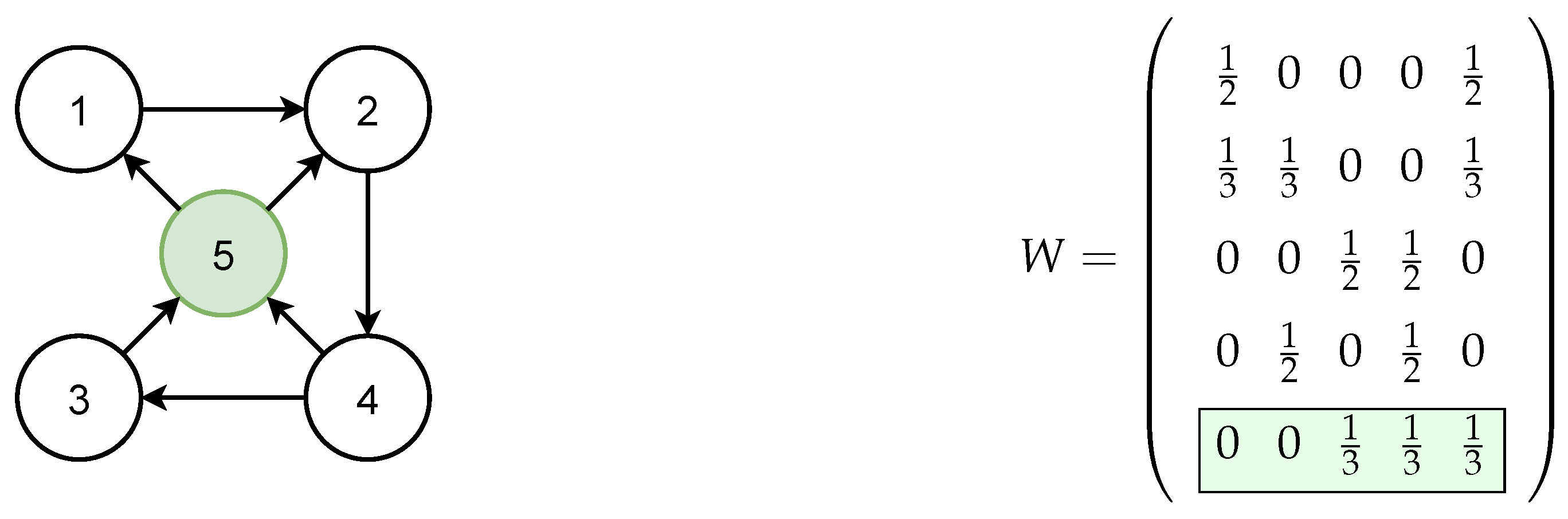
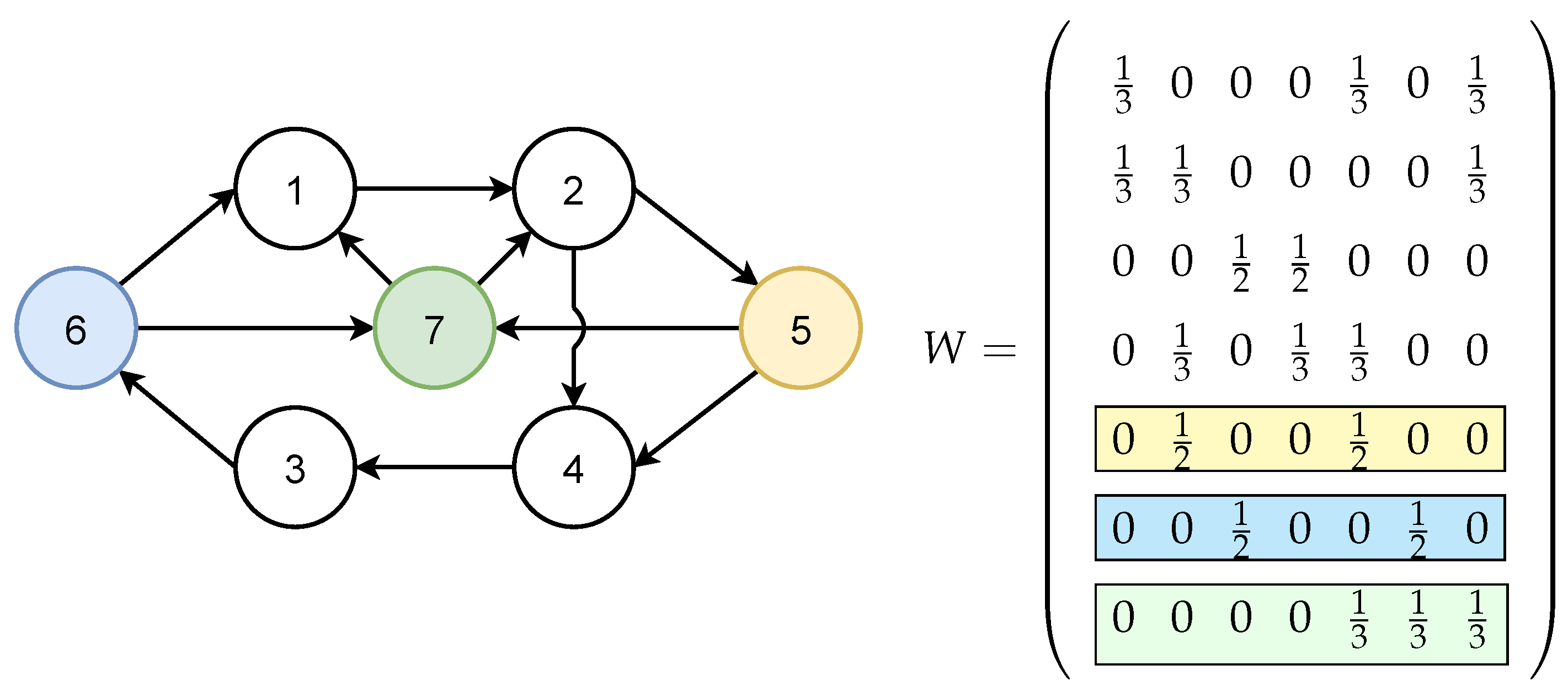
Next, it will be focused on the procedure for constructing the weight matrix W.

Definition 2. 

For all $i\in O_{c,s,w,b}$ and $\kappa \ge 0$ one can define a positive scalar $\kappa \in (0,1)$ for which:

$$\begin{array}{c}\hfill w_{ij}=\left\{\begin{array}{c}>\kappa ,j\in \mathcal{G}\bigcup i,\hfill \\ \\ 0\mathit{otherwise}.\hfill \end{array}\right.\end{array}$$

(28)

At the same time, the values of $w_{ij}$ must hold ${\sum }_{j=1}{w}_{ij}=1$ for a given row of the weight matrix W.

From now on, it is essential to note that the indices i and j represent all types of power plants, including conventional, renewables, and BESS. The $\kappa$ lower bound ensures that the information link between agents i and j will not be too weak. Furthermore, in line with Definition 2, the entire weight matrix W associated with the graph $\mathcal{G}$ is row stochastic $W=\left[w_{ij}\right]\in R^{N\times N}$ and $W{1}_N$.

Each generation unit $i\in O_{c,s,w,b}$ only requires its local information, denoted as $d_i^{in}$ (the number of incoming edges), to construct the row-stochastic weight matrix W. Each agent can independently determine $d_i^{in}$ value without needing information from its neighbors.

In order to fulfill this requirement, the values for $w_{ij}$ should be chosen according to:

$$\begin{array}{c}\hfill w_{ij}=\left\{\begin{array}{c}\frac{1}{d_i^{in}+1},j\in \mathcal{G}\bigcup i,\hfill \\ \\ 0.\mathrm{otherwise}.\hfill \end{array}\right.\end{array}$$

(29)

In this case, Definition 2 is satisfied by choosing $\kappa =\frac{1}{N}$.

Next, it will be moved to the shape of the ${\Phi }_i\left({\lambda }_i\right)$ gradient calculation. The gradient of ${\Phi }_i\left({\lambda }_i\right)$ calculation have following shape:

$$\begin{array}{c}\hfill \nabla {\Phi }_i\left({\lambda }_i\right)=P_i\left({\lambda }_i\right)-P_{D_i}.\end{array}$$

The variable ${\Phi }_i\left({\lambda }_i\right)$ is bounded from above due to the sum of maximum possible power $P_i$ and virtual required loads $P_{D_i}$ across all generators:

$$\begin{array}{c}\hfill |\nabla {\Phi }_i\left({\lambda }_i\right)|=|P_i\left({\lambda }_i\right)-P_{D_i}|\le \underset{i\in \mathcal{G}}{max}{P}_i^{max}+\underset{i\in \mathcal{G}}{max}{P}_{D_i}.\end{array}$$

The variable $P_{D_i}$ indicates a virtual local demand with no physical meaning. It is used only for the ability to build a distributed algorithm. Thus, $P_{D_i}$ values can be chosen randomly across all agents in the network only under the condition that their sum corresponds to the required load $P_D$ to meet the condition stated in (34) [8].

In the article [62], it is stated that the standard gradient method without weighting by the term $y_{ii}$ can only lead to the minimization of the term ${\sum }_{i=1}^N{\pi }_i{\Phi }_i\left(\lambda \right),$ instead of term ${\sum }_{i=1}^N{\Phi }_i\left(\lambda \right)$, especially for the reason of unbalancedness of directed graph. Here ${\pi }_i\in (0,1)$ applies where it is the i-th member of the vector $\pi ={[{\pi }_1,\dots ,{\pi }_N]}^T\in R^N$. It is, therefore, a left-normalized vector of eigenvalues (Perron vector) of the matrix W that satisfies:

$$\begin{array}{c}\hfill \underset{k\to +\infty }{lim}{W}^k=1_N{\pi }^T,\mathrm{and}{1}_N^T\pi =1.\end{array}$$

The vector $\pi$, sometimes called the “Perron vector”, is relevant in the context of the “Perron–Frobenius Theorem” (The Perron–Frobenius Theorem stated that a real square matrix with positive entries has a unique largest real eigenvalue and that the corresponding eigenvector can be chosen to have strictly positive components, and then a similar statement for certain classes of non-negative matrices. This Theorem has essential applications to probability theory, theory of dynamical systems, economics, and many more.) Computing this vector in advance would enable scaling the gradient by it. However, determining the Perron vector in advance is challenging since the algorithm cannot perform this step until each generator knows its local ${\pi }_i$. To address this, the variable $y_i\left(k\right)$ is introduced for asymptotic estimation of the Perron vector.

The re-scaling gradient technique was initially introduced in [63]. It is essential to note that one requirement for this method to function correctly is that each generator knows the total required network load $P_D$. Knowledge of $P_D$ can be ensured through a strongly connected graph, information transmission, and unique identifiers for each generator.

Now, let us delve into the calculation for the quadratic price function, which applies to conventional generators and is the most complex part. In (23), the argument of the $\phi$ function involving $\nabla C_{c_i}^{-1}\left({\lambda }_{c_i}(k+1)\right)$ does not have a closed-form solution for a universal convex cost function. Moreover, for ${\phi }_i\left(\nabla C_{c_i}^{-1}\left({\lambda }_{c_i}(k+1)\right)\right)$, will be received:

$$\begin{array}{c}\hfill {\phi }_{c_i}\left(C_{c_i}^{-1}\left({\lambda }_{c_i}(k+1)\right)\right)=\left\{\begin{array}{cc}{P}_{c_i}^{max},\hfill & \mathrm{if}{C}_{c_i}^{-1}\left({\lambda }_{c_i}\left(k\right)\right)>P_{c_i}^{max},\hfill \\ \\ \nabla C_{c_i}^{-1}\left({\lambda }_{c_i}\left(k\right)\right),\hfill & \mathrm{if}{P}_{c_i}^{min}\le C_{c_i}^{-1}\left({\lambda }_{c_i}\left(k\right)\right)\le P_{c_i}^{max},\hfill \\ \\ P_{c_i}^{min},\hfill & \mathrm{if}{C}_{c_i}^{-1}\left({\lambda }_{c_i}\left(k\right)\right)<P_{c_i}^{min}.\hfill \end{array}\right.\end{array}$$

If a quadratic price function of $C_{c_i}$ (21) is considered then $\nabla C_{c_i}^{-1}\left({\lambda }_{c_i}\right)$ has form:

$$\begin{array}{c}\hfill \nabla C_{c_i}^{-1}\left({\lambda }_{c_i}\right)={\beta }_{c_i}{\lambda }_{c_i}+{\alpha }_{c_i},\end{array}$$

where ${\alpha }_{c_i}$ and ${\beta }_{c_i}$ are parameters of the i-th conventional generator.

Similarly, renewable sources and BESS, which have maximum energy limits, can be constrained by ${\phi }_{{s,w}_i}$ or ${\phi }_{b_i}$. In the case of BESS, this function also includes deciding whether to provide power to the grid or store it, denoted as the $\mathsf{{\rm Y}}\left(\right)$ decision function.

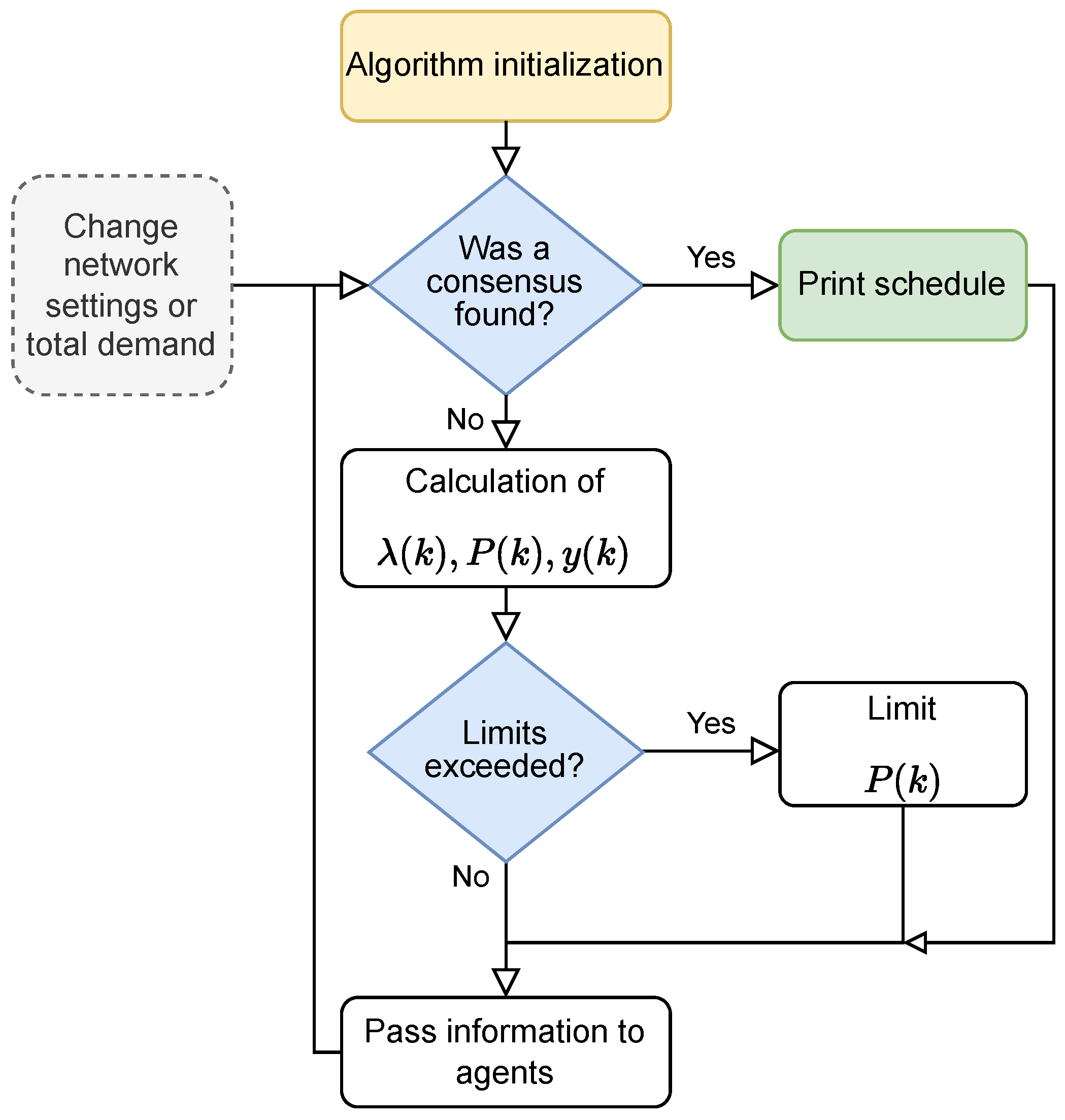
4.4.1. Sequence of Operations for Deploying the Algorithm

The possible implementation of the described algorithm will be outlined here in a very simple way. A simplified flowchart of the operations sequence with the presented algorithm is shown in Figure 4. The entire process runs in a continuous loop. The calculation block contains the calculation of the Equations of the algorithm (22)–(24). The yellow block indicates the starting initialization. Finding a consensus means that all online agents in the network have reached the same value of ${\lambda }_i\left(k\right)$. If the convergence has been achieved then the production plan can be passed to the individual generators, which is represents by green block. The gray block represents changes in the network settings, desired load, or other inputs from other agents. These modifications can lead to a change in the ${\lambda }_i\left(k\right)$ value or the local requirements of $P_{D_i}$, and the entire algorithm is thus recalculated.

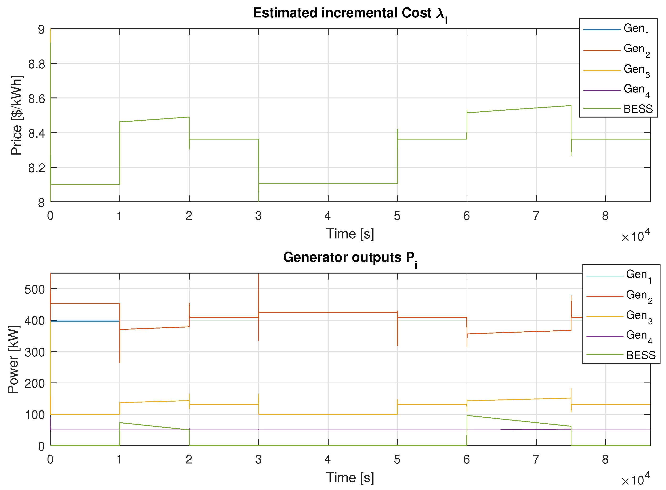
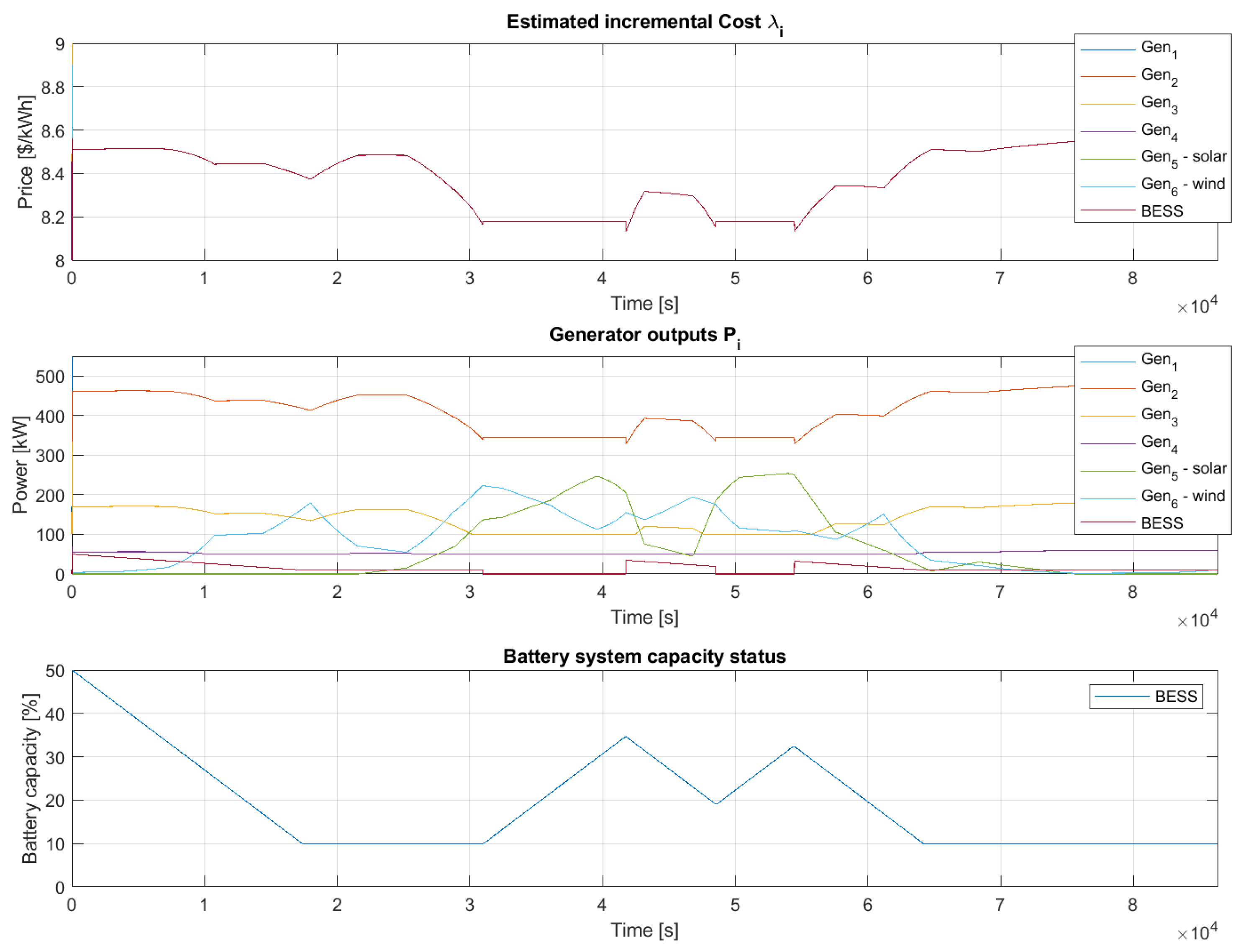
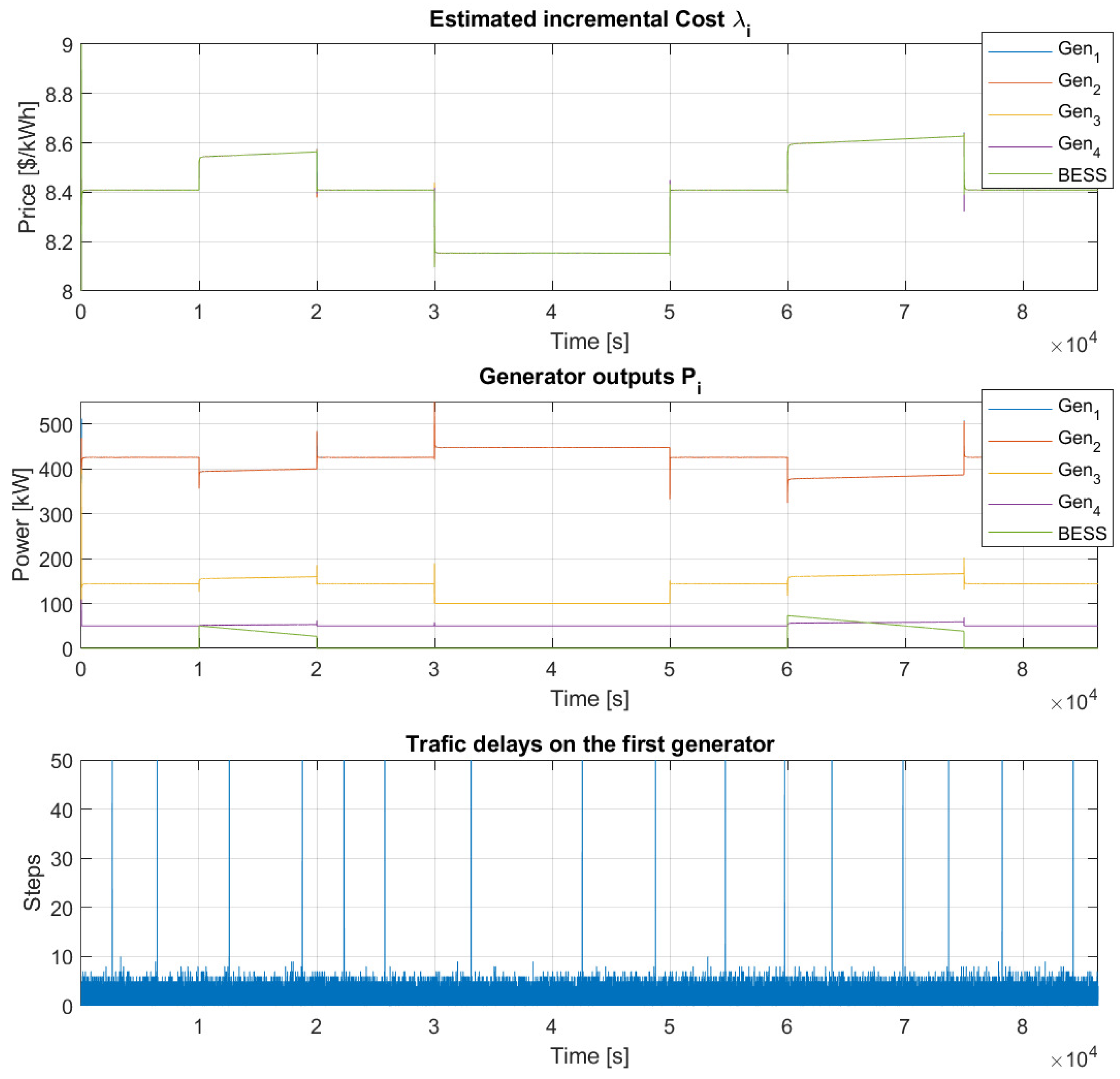
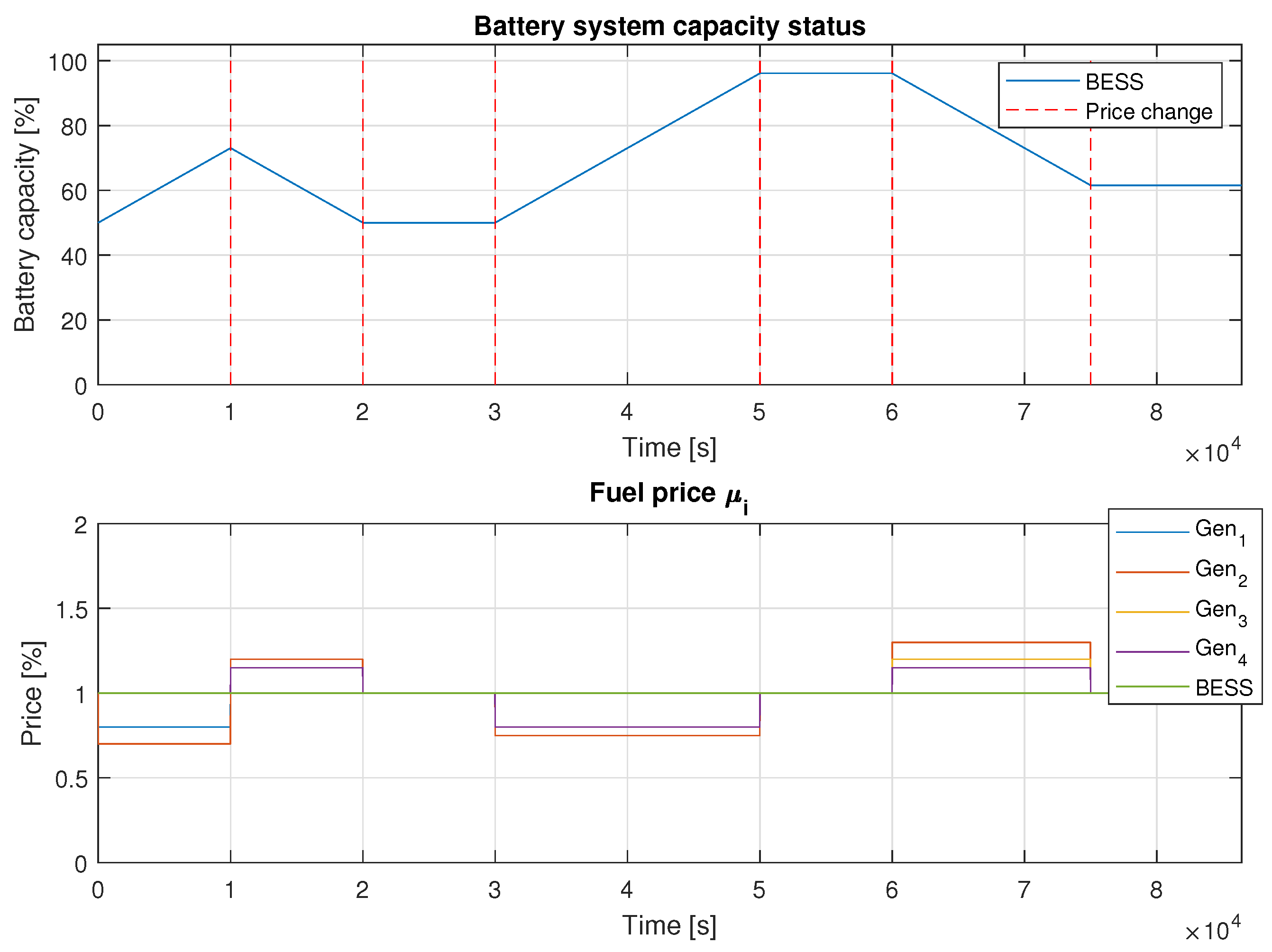
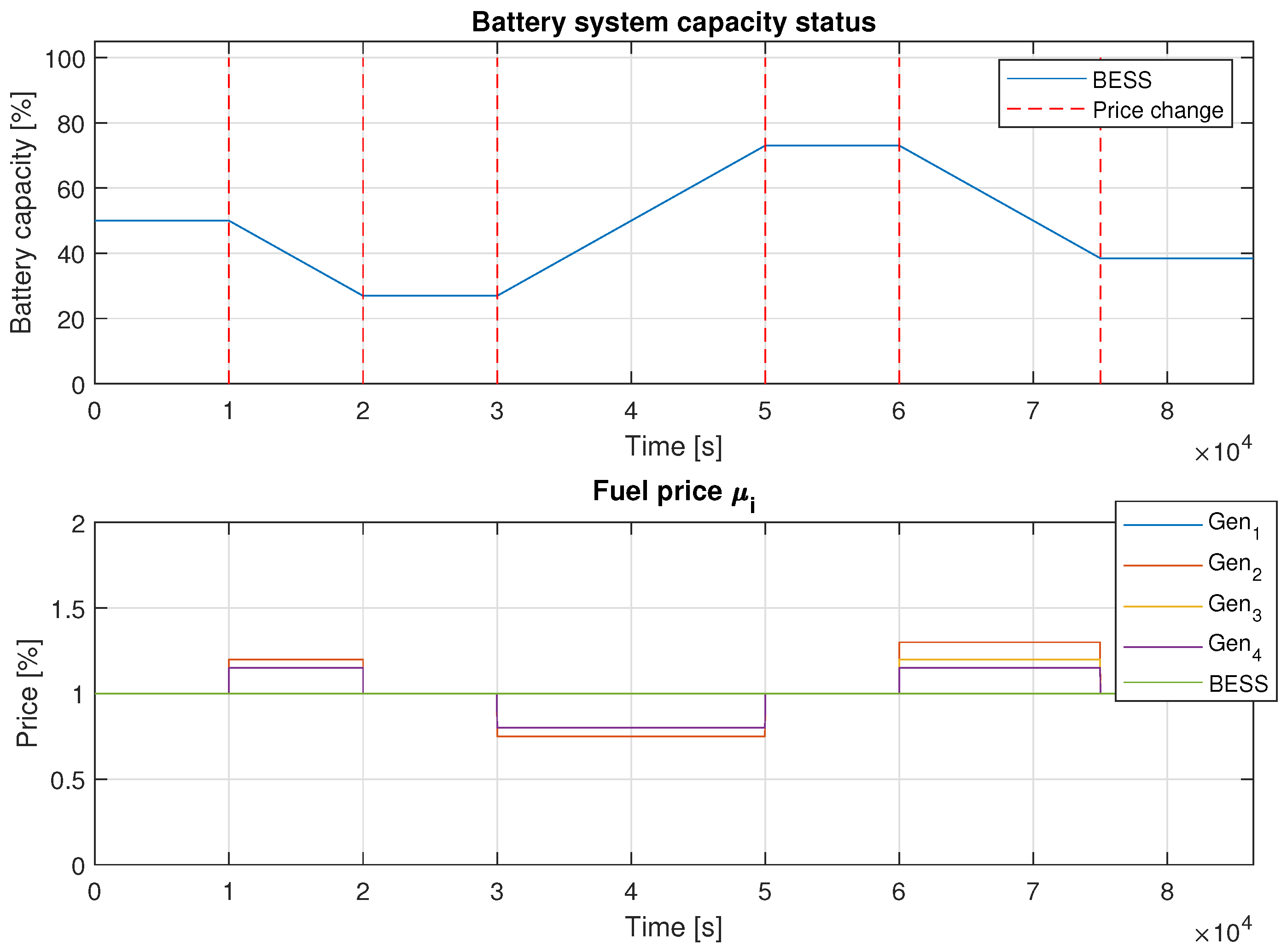
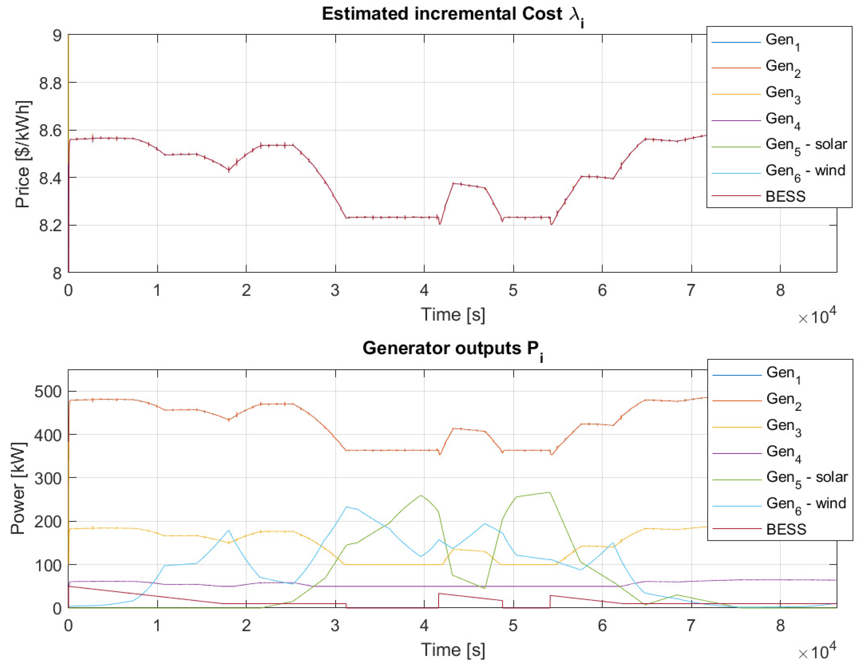
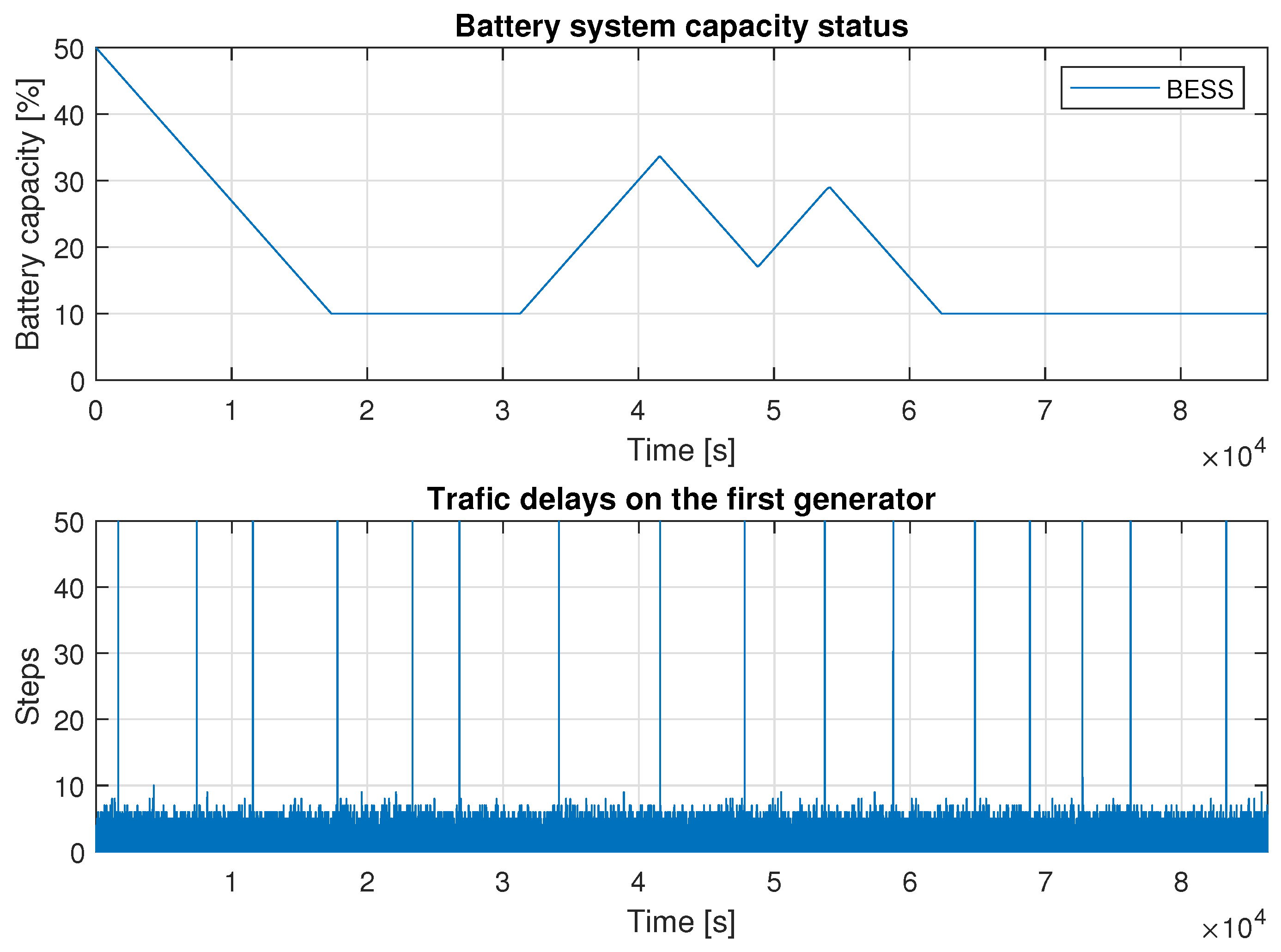
At this place it is important to mention that the entire algorithm runs online and thus reacts to any changes in the input information itself. This fact will be further demonstrated by examples in Section 5. The aim of this analysis is to provide better insight into the possible integration of the presented algorithm.

4.4.2. Convergence Analysis

In this section, the analysis of convergence for the algorithm will be conducted. Before delving into the convergence analysis, it is essential to establish specific facts about the directed graph $\mathcal{G}$ and the weight matrix W. The subsequent Lemmas and Theorems will be stated generically using the index i, ensuring their applicability to all source types.

Lemma 1. 

Definitions 1 (Equation (25)) and 2 (Equation (28)) hold for the graph $\mathcal{G}$ and the matrix W. Parameter ${\pi }_i$ is left normalized eigenvalues vector of the matrix W. Then there exists a parameter $\beta \le 0$ and $\xi \in (0,1)$ such that $\forall i,j\in \mathcal{G}$ and $k\ge 0$, it holds that [63]:

$$\begin{array}{c}\hfill |{\left[W^k\right]}_{ji}-{\pi }_i|\le \beta {\xi }^k,|y_{ii}\left(k\right)-{\pi }_i|\le \beta {\xi }^k.\end{array}$$

Furthermore, a constant $h>1$ will be introduced such that:

$$\begin{array}{c}\hfill h^{-1}\le y_{ii}\left(k\right)\le 1,\forall i,j\in \mathcal{G},k\ge 0.\end{array}$$

This Lemma will subsequently be used to establish results for asymptotic consensus.

Lemma 2. 

In this Lemma, the following sequence will be introduced [63]:

$$\begin{array}{c}\hfill {\theta }_i(k+1)=\sum _{j=1}^N{w}_{ij}{\theta }_j\left(k\right)+{ϵ}_i\left(k\right).\end{array}$$

Here, Definition 1 still holds for $w_{ij}$. Subsequently, a variable $\overline{\theta }\left(k\right)$ will be introduced:

$$\begin{array}{c}\hfill \overline{\theta }\left(k\right)=\sum _{i=1}^N{\pi }_i{\theta }_i\left(k\right).\end{array}$$

where the parameter ${\pi }_i$ was defined in Lemma 1. Furthermore, if it is considered that ${lim}_{k\to +\infty }\left|\right|{ϵ}_i\left(k\right)\left|\right|=0$ then:

$$\begin{array}{c}\hfill \underset{k\to +\infty }{lim}\left|\right|{\theta }_i\left(k\right)-\overline{\theta }\left(k\right)\left|\right|=0,\forall i\in \mathcal{G}.\end{array}$$

In this Lemma, the deterministic counterpart to the supermartingale convergence Theorem is thus relied upon to achieve asymptotic convergence for the dual variable ${\lambda }_i\left(k\right)$. (Doob’s martingale convergence Theorems, named after mathematician Joseph L. Doob, deal with the limits of supermartingales. Supermartingales are like decreasing sequences in the world of random variables. The main idea is that, under certain conditions, a supermartingale will always converge. This Theorem is akin to the monotone convergence Theorem, which tells us that bounded decreasing sequences converge.)

Lemma 3. 

In the next step, a non-negative scalar sequence $\left\{s\right(k\left)\right\}$ will be introduced for $\forall k\ge 0$ such that it satisfies [64]:

$$\begin{array}{c}\hfill s(k+1)\le \left(1+v\left(k\right)\right)·s\left(k\right)-b\left(k\right)+c\left(k\right),\end{array}$$

(30)

where for the parameters $v\left(k\right),b\left(k\right),c\left(k\right)\ge 0$ with the condition for $v\left(k\right)$ and $c\left(k\right)$:

$$\begin{array}{c}\hfill \sum _{k=0}^{\infty }v\left(k\right)<\infty ,\sum _{k=0}^{\infty }c\left(k\right)<\infty .\end{array}$$

It follows that ${lim}_{k\to +\infty }s\left(k\right)=\sigma$, where σ is a non-negative constant for which $\sigma \ge 0$ and at the same time ${\sum }_{k=0}^{\infty }b\left(k\right)<\infty$.

Lemma 4. 

(Asymptotic consensus) Here, it will be returned to the algorithm defined by the Equations (22)–(24). Furthermore, it will be assumed that Assumptions 1–3 and Definitions 1 and 2 still hold true. Subsequently, a variable $\overline{\lambda }\left(k\right)$ will be introduced [8]:

$$\begin{array}{c}\hfill \overline{\lambda }\left(k\right)=\sum _{i=1}^N{\pi }_i{\lambda }_i\left(k\right).\end{array}$$

Then the form for the limit can be written as:

$$\begin{array}{c}\hfill \underset{k\to +\infty }{lim}\left|\right|\lambda \left(k\right)-\overline{\lambda }\left(k\right)\left|\right|=0,\mathrm{for}\mathrm{any}i\in \mathcal{G}.\end{array}$$

This results in the convergence of $\overline{\lambda }\left(k\right)$ to the optimal value reached by all agents in the network. Proof can be found in Appendix A.

Lemma 5. 

It will be assumed that Assumptions 1–3 and Definitions 1 and 2 hold true again. Consequently, for any $u\in R$ and $k\ge 0$, the following holds [8]:

$$\begin{array}{c}\hfill \begin{array}{c}\hfill \sum _{i=1}^N{\pi }_i\left|\right|{\lambda }_i(k+1)-{u\left|\right|}^2\le \sum _{i=1}^N{\pi }_i\left|\right|{\lambda }_i\left(k\right)-u{\left|\right|}^2-\frac{2}{k+1}(\Phi (\overline{\lambda }\left(k\right)-\Phi \left(u\right)))\\ \hfill +\frac{6lh}{k+1}\sum _{i=1}^N{\pi }_i\left|\right|{\lambda }_i\left(k\right)-\overline{\lambda }\left(k\right)\left|\right|+2lha\left(k\right)\sum _{i=1}^N{\pi }_i\left|\right|{\lambda }_i\left(k\right)-u\left|\right|+h^2{l}^2\sum _{i=1}^N{\pi }_i{\gamma }_i^2\left(k\right)\\ \hfill +\frac{2nh\beta {\xi }^k}{k+1}\left|\right|{\overline{\lambda }}_i\left(k\right)-u\left|\right|.\end{array}\end{array}$$

(31)

Proof can be found in Appendix B.

Lemma 6. 

Renewable sources cannot be controlled. Their operation is thus directly dependent on the current weather, as stated in Assumption 1. However, if their electricity production is available, it can be decided whether and in what quantity it will be consumed locally, provided to the grid, stored in battery systems or unused. In the case of using all the provided energy, this can be imagined as a change in the value of the required load $P_D$ for the entire system:

$$\begin{array}{c}\hfill \sum _{i=1}^{N_c}{P}_{c_i}+\sum _{i=1}^{N_b}{P}_{b_i}+P_g=\left(P_D-\sum _{i=1}^{N_s}{P}_{s_i}-\sum _{i=1}^{N_w}{P}_{w_i}\right).\end{array}$$

Thus, the entire right side can be marked as $P_{D_{{\mathit{new}}_1}}$, which represents the reduced value of the total required load D by renewable resources:

$$\begin{array}{c}\hfill \sum _{i=1}^{N_c}{P}_{c_i}+\sum _{i=1}^{N_b}{P}_{b_i}+P_g=P_{D_{{\mathit{new}}_1}}.\end{array}$$

Similarly, based on the current needs and requirements, the claim could be modified only for partial use of the total power provided by renewable sources or its partial storage in the BESS.

Lemma 7. 

Similar to the Lemma 6 BESSs can either provide energy to the local network in island mode (discharge), to the grid (discharge), absorb it from local assets or from the grid (charge). Their state depends on the upcoming input, which determines their operation. This decision-making process relies on specific design and logic.

In the case of using energy from BESS or storing the energy to the BESS, change to the $P_D$ can be written as:

$$\begin{array}{c}\hfill \sum _{i=1}^{N_c}{P}_{c_i}+\sum _{i=1}^{N_s}{P}_{s_i}+\sum _{i=1}^{N_w}{P}_{w_i}+P_g=\left(P_D-\sum _{i=1}^{N_b}{P}_{b_i}\right),\end{array}$$

where a new value of the total required load $P_{D_{{\mathit{new}}_2}}$ can be introduced again, which will increase or decrease the original value of $P_D$ depending on whether the BESS is being discharged or charged:

$$\begin{array}{c}\hfill \sum _{i=1}^{N_c}{x}_{c_i}+\sum _{i=1}^{N_s}{x}_{s_i}+\sum _{i=1}^{N_w}{x}_{w_i}+P_g=P_{D_{{\mathit{new}}_2}}.\end{array}$$

Remark 4. 

If the connection to the grid is ensured, $P_g$ will be preserved and used in the equations. If the island mode of the local network is considered, then the term $P_g$ will be considered as zero.

Based on all the mentioned Lemmas, Theorem 1 can be constructed.

Theorem 1. 

Let Assumptions 1–3 and Definitions 1 and 2 hold true. Then the algorithm stated in (22)–(24) solves the problem defined in Section 3 in Equation (2)–(4). This can be written as for $k\to \infty$ applies:

$$\begin{array}{c}\hfill {\lambda }_i\left(k\right)\to {\lambda }^{*},P_i\left(k\right)\to P^{*},\forall i\in \mathcal{G},\end{array}$$

(32)

where variable ${\lambda }^{*}$ represents optimal incremental cost and $P^{*}$ denotes optimal power generation for each i-th generator in the graph $\mathcal{G}$. It follows that the algorithm converges to the optimal solution. Proof can be found in Appendix C.

From Lemma 6 and Lemma 7, it becomes evident that renewables generate power according to weather conditions. At the same time, BESSs can supply or draw power from the grid through a control function both in island mode and when connected to the grid.

4.4.3. Zero Cost for Renewables

In the case of the considered zero fuel price $C_{s_i}$ and $C_{w_i}$ for renewable sources, the calculation of the Equation for (22) for ${\lambda }_i(k+1)$ will be changed. The remaining two Equations (23) and (24) remain unchanged.

$$\begin{array}{cc}\hfill {\lambda }_i(k+1)& =\sum _{j=1}^N{w}_{ij}{\lambda }_j\left(k\right)-\left\{\begin{array}{cc}{\gamma }_i\left(k\right)\frac{\nabla {\Phi }_i\left({\lambda }_{c_i}\left(k\right)\right)}{y_{ii}\left(k\right)},\hfill & \mathrm{if}i\in O_c\hfill \\ \\ 0,\hfill & \mathrm{if}i\in O_{s,w}\hfill \\ \\ {\gamma }_i\left(k\right)\frac{\nabla {\Phi }_i\left({\lambda }_{b_i}\left(k\right)\right)}{y_{ii}\left(k\right)},\hfill & \mathrm{if}i\in O_b\hfill \end{array}\right.\hfill \end{array}$$

(33)

This adjustment can be afforded because the price for solar or wind energy is zero, and its availability depends only on the weather. This simplification will also be used in Section 5 in the simulation examples.

4.5. Algorithm with Multiple Uncertainties

This section will enhance the algorithm presented earlier to address various uncertainties concurrently, including line losses, imprecise gradient calculations, time-varying traffic delay, and representation of drop-off packets [49].

4.5.1. Line Losses

Line losses cannot be avoided when transporting energy using cables over long distances. In addition, each voltage transformation to another level also brings with it certain losses. Line losses will be marked as $P_{\mathrm{loss}}$ and are added to the total required load $P_D$. This will compensate them. Formula (3) then takes the form:

$$\begin{array}{c}\hfill \sum _{i=1}^{N_c}{P}_{c_i}+\sum _{i=1}^{N_s}{P}_{s_i}+\sum _{i=1}^{N_w}{P}_{w_i}+\sum _{i=1}^{N_b}{P}_{b_i}+P_g=P_D+P_D·P_{\mathrm{loss}}.\end{array}$$

(34)

Line losses are minimal compared to the load in the networks. That is why they are often neglected in EDP [10], but to obtain a more accurate model it is advisable to consider them. These losses are often thought of as 5% ($0.05$) of the total demand $P_D$ [13]:

$$\begin{array}{c}\hfill P_D=P_D+P_D·P_{loss}=P_D·(1+P_{loss})=P_D·(1+0.05)=1.05·P_D.\end{array}$$

Moreover, subsequently, the same rule will apply to the individual local demands $P_{D_i}$:

$$\begin{array}{c}\hfill P_{D_i}=P_{D_i}+P_{D_i}·P_{loss}=P_{D_i}·(1+P_{loss})=P_{D_i}·(1+0.05)=1.05·P_{D_i}.\end{array}$$

This modification is reflected in the initialization of the algorithm for $P_i\left(0\right)$:

$$\begin{array}{cc}\hfill P_i\left(0\right)& =\left\{\begin{array}{cc}{P_i}^{\max }\hfill & \mathrm{if}{P_i}^{\max }<P_{D_i},\hfill \\ \\ D_i\hfill & \mathrm{if}{P_i}^{\min }\le P_{D_i}\le {P_i}^{\max },\hfill \\ \\ {P_i}^{\min }\hfill & \mathrm{if}{P}_{D_i}<{P_i}^{\min },\hfill \end{array}\right.\forall i\in N.\hfill \end{array}$$

4.5.2. Noisy Gradient Calculation

The noisy gradient calculation means that the generator does not require the exact gradient value but a noisy version. This noise can arise from measurement errors or fluctuations in the energy network. A label for the observation noise ${\nu }_i\left(k\right)$ will be introduced for the i-th generator in the network at step k. The noise affects the algorithm solely in the equation for ${\lambda }_i(k+1)$ to calculate the gradient:

$$\begin{array}{cc}\hfill {\lambda }_i(k+1)& =\sum _{j=1}^N{w}_{ij}{\lambda }_j(k-{\tau }_{ji})-{\gamma }_i\left(k\right)\frac{\nabla {\Phi }_i\left({\lambda }_i\left(k\right)\right)+{\nu }_i\left(k\right)}{y_{ii}\left(k\right)}.\hfill \end{array}$$

Next, the $\delta$-algebra $F_k$ will be introduced. (A delta-algebra includes sets that remain closed under countable intersections. In simpler terms, if you have many sets in the delta-algebra, their intersection will also belong to it. Delta-algebras are a broader version of $\sigma$-algebras, encompassing sets closed under countable unions and intersections. The key difference is that a delta-algebra does not have to include sets necessarily closed under countable unions.) This will be generated by the entire running history of the algorithm up to the $k–$th iteration. Then the noise ${\nu }_i\left(k\right)$ is bounded by the zero-mean noise variance:

$$\begin{array}{c}\hfill E\left[{\nu }_i\left(k\right)\right|F_{k-1}]=0,E\left[{\nu }_i^2\left(k\right)\right|F_{k-1}]\le {\widehat{\nu }}^2,\end{array}$$

where $\widehat{\nu }>0$ for all agents in the network and $k\ge 0$.

4.5.3. Time-Varying Traffic Delay

In real applications, traffic delays are inevitable when many agents communicate with each other. It will be noted that ${\tau }_{ji}$ represents the unknown traffic delay on the communication line from agent i to agent j. Traffic delay ${\tau }_{ji}$ can be modeled using normal random distribution where $\omega$ denotes the mean value and ${\sigma }^2$ represents the variance.

$$\begin{array}{c}\hfill {\tau }_{ji}\left(k\right)\sim \mathcal{N}(\omega ,{\sigma }^2)\end{array}$$

It is assumed that the traffic delay is uniformly bounded, which means that there exists a positive value of ${\tau }_{\max }$ for which:

$$\begin{array}{c}\hfill 0\le {\tau }_{ji}\left(k\right)\le {\tau }_{\max },j\in {\mathcal{N}}_i^{in},\end{array}$$

(35)

where ${\tau }_{ii}=0,\forall i$ in graph $\mathcal{G}$.

One can imagine that the traffic delay cannot be negative. Therefore, the term log-normal distribution can sometimes be encountered. That is why its absolute value is then used for the following calculations. Since it is a discrete iterative algorithm, traffic delays can be integer values only. Unfortunately, normal distribution also returns decimal numbers. Therefore, the round function is used here, assuring that the result will be an integer. The resulting value is used for all generators in a given time step.

$$\begin{array}{c}\hfill {\tau }_{ji}\left(k\right)\sim \mathrm{round}\left(\left|\mathcal{N}\right(\omega ,{\sigma }^2\left)\right|\right)\end{array}$$

4.5.4. Drop-Off Packet Representation

The term “drop-off packet’,’ also known as a “lost packet”, is commonly used in communication scenarios. It can be modeled using the Bernoulli process, denoted as $X\sim Ber\left(p\right)$. The Bernoulli process is a discrete-time stochastic process involving binary random variables, taking either 0 or 1 values. Specifically, it is characterized by $P(X=1)=p$ and $P(X=0)=(1-p)$.

An alternative model can be Binomial distribution. Binomial distribution means the instance frequency of a random event in N independent trials. The probability can be formulated as $X\sim Bi(n,p)$. Parameter n represents the number of attempts, and parameter p denotes the probability. Binomial distribution thus describes that the event will occur x times out of a total of n attempts, with a probability of p.

$$\begin{array}{c}\hfill P[x=X]=\left(\left(\genfrac{}{}{0pt}{}{n}{x}\right)\right)p^x(1-p)p^{n-x}\end{array}$$

The mean is represented by E, and the variance is marked as D. They can be expressed as:

$$\begin{array}{c}\hfill E\left[X\right]=np,D\left[X\right]=np(1-p).\end{array}$$

The Binomial distribution thus works with the result for multiple trials for a given event. In contrast, the Bernoulli process is used if the result is needed only once. This means that Bernoulli is designed for the outcome of a single trial for the given event.

If the traffic delay approaches infinity or some invalid value, this state can be labelled as a Drop-off packet.

$$\begin{array}{c}\hfill \text{drop-off}\text{packet}:{\tau }_i\left(k\right)\to \infty \end{array}$$

If the traffic delay ${\tau }_i\left(k\right)$ has a constant value lower than the limit given in (35), then the algorithm converges, as was shown in [65]. However, the traffic delay can take on values higher than this limit, which makes it possible to add the representation and treatment of these events. In case that the traffic delay ${\tau }_i\left(k\right)$ rises above limit value ${\tau }_{\max }+1$, then it can be marked as a Drop-off packet.

$$\begin{array}{cc}\hfill {\tau }_i\left(k\right)& =\left\{\begin{array}{cc}{\tau }_i\left(k\right)\hfill & \mathrm{if}{\tau }_i\left(k\right)<{\tau }_{\max }+1\hfill \\ \\ \infty \hfill & \mathrm{if}{\tau }_i\left(k\right)\ge {\tau }_{\max }+1\hfill \end{array}\right.\hfill \end{array}$$

From the Equation (37)–(39) is clear that the traffic delay only affects the calculation of the Equations for $\lambda$ (37) and y (39).

$$\begin{array}{cc}\hfill {\lambda }_i\left(k\right)& =\left\{\begin{array}{cc}{\lambda }_i\left(k\right)\hfill & \mathrm{if}{\tau }_i\left(k\right)\ne \infty \hfill \\ \\ {\lambda }_i(k-1)\hfill & \mathrm{if}{\tau }_i\left(k\right)=\infty \hfill \end{array}\right.\hfill \end{array}$$

(36)

The same rule shown in (36) applies to $y_i\left(k\right)$, substituting $\lambda$ by y. This straightforward adjustment effectively addressed oscillations and instability caused by significant traffic delays. It also prevented potential issues, such as fatal collapse, if negative indices were involved in the discrete algorithm.

With the provided insights, these elements can be integrated into the existing algorithm expressed by Equations (22)–(24). The modified algorithm version will take the following form:

$$\begin{array}{cc}\hfill {\lambda }_i(k+1)& =\sum _{j=1}^N{w}_{ij}{\lambda }_j(k-{\tau }_{ji})-\left\{\begin{array}{cc}{\gamma }_i\left(k\right)\frac{\nabla {\Phi }_i\left({\lambda }_{c_i}\left(k\right)\right)+{\nu }_i\left(k\right)}{y_{ii}\left(k\right)},\hfill & \mathrm{if}i\in O_c,\hfill \\ \\ 0,\hfill & \mathrm{if}i\in O_{s,w},\hfill \\ \\ {\gamma }_i\left(k\right)\frac{\nabla {\Phi }_i\left({\lambda }_{b_i}\left(k\right)\right)+{\nu }_i\left(k\right)}{y_{ii}\left(k\right)},\hfill & \mathrm{if}i\in O_b,\hfill \end{array}\right.\hfill \end{array}$$

(37)

$$\begin{array}{cc}\hfill P_i(k+1)& =\left\{\begin{array}{cc}{\phi }_{c_i}\left(\nabla C_{c_i}^{-1}({\lambda }_{c_i}(k+1)·{\mu }_{c_i}^{-1}\left(k\right))\right),\hfill & \mathrm{if}i\in O_c,\hfill \\ \\ {\phi }_{{s,w}_i}\left(P_{{s,w}_i}·{\mu }_{{s,w}_i}\left(k\right)\right),\hfill & \mathrm{if}i\in O_{s,w},\hfill \\ \\ {\phi }_{b_i}\left(\mathsf{{\rm Y}}\left(E_{b_i}\left(t\right)\right)·{\mu }_{b_i}\left(k\right)\right),\hfill & \mathrm{if}i\in O_b,\hfill \end{array}\right.\hfill \end{array}$$

(38)

$$\begin{array}{cc}\hfill y_i(k+1)& =\sum _{j=1}^N{w}_{ij}{y}_j(k-{\tau }_{ji}).\hfill \end{array}$$

(39)

Theorem 2 will be presented in the next step, which describes that the algorithm represented by Equations (37)–(39) is robust against all the inaccuracies described above and still converges to the optimal solution.

Theorem 2. 

Assumptions 1–3 and Definitions 1 and 2 still hold again. Then the algorithm stated in (37)–(39) solves then problem defined in Section 3 in Equations (2)–(4) with all described uncertainties and satisfying conditions (35) and (36). This can be written as for $k\to \infty$ applies:

$$\begin{array}{c}\hfill \underset{k\to \infty }{lim}{\lambda }_i\left(k\right)\to {\lambda }^{*},\underset{k\to \infty }{lim}{P}_i\left(k\right)\to P^{*},\forall i\in \mathcal{G},\end{array}$$

where variable ${\lambda }^{*}$ represents optimal incremental cost value and $P^{*}$ denotes optimal power generation for each i-th generator in the graph $\mathcal{G}$. Proof can be found in Appendix D.

5. Simulation Examples

This section will introduce simulation examples that illustrate the capabilities and applications of the presented algorithm. Six examples will be divided into two parts, each comprising three scenarios. The examples were implemented in the Matlab program using the model-based design approach, widely used in practice [66].

The first part will focus on using the algorithm without uncertainties, while the second part will include the same examples but with additional uncertainties. This allows for a direct comparison of the results. Detailed information for replicating these examples will be provided. Next, the zero price of renewable resources will be considered (Equation (33)). For further simplification, the term $P_g$ given in Equations (2) and (3) will be assumed to be zero, which was discussed in Remark 4. Thus, only the island mode will be considered. As a result, its price function will also be zero. However, it is not a problem to implement this agent in the network as another node, which will either provide additional power taken from the extensive network or increase the total required load $P_D$ of the local network.

5.1. Examples with No Consideration of Uncertainties

In this part, the focus will be on using the algorithm without respecting multiple uncertainties at once. The first example covers the required network load, i.e., convergence to the optimal solution. The second example focuses on incorporating a BESS into a grid topology while considering a variable cost function. The third example combines both of the above using real weather forecast data. The learning gains $\gamma$ will be represented as a constant in examples without uncertainties. Its value is calculated according to (27) at the beginning.

5.1.1. Example 1—Coverage of the Required Load and Its Changes

The algorithm will be presented by example, comprising four generators and two renewable power plants. One will be a large solar power plant, and the other will be a wind power plant. Three types of generators will be introduced. First will be Type I represents coal-fired steam unit, then Type II is oil-fired steam unit and Type III denotes oil-fired steam unit. The generator parameters were adapted from [10] only with the difference that the power of the generators will be considered in kW. Their values are described in

Table 1. Generator parameters.

Generation Unit Parameters
Generator Type	Type I	Type II	Type III
Range [kW]	[$150,600$]	[$100,400$]	[$50,200$]
$\alpha$ [USD/${\mathrm{kW}}^2\mathrm{h}$]	$-2535.211268$	$-2023.195876$	$-826.7634855$
$\beta$ [USD/kWh]	$352.1126761$	$257.7319588$	$103.7344398$
$\gamma$ [USD/h]	$-8616.760563$	$-7631.043814$	$-3216.65249$

.

The total demand will be set as $P_D=1500$ kW. Local demands $P_{D_i}$ will be set randomly between all agents, with the condition that their sum must be equal to $P_D$.

Table 2. Initialization of $P\left(0\right),y\left(0\right),\lambda \left(0\right),P_D\left(0\right),M\left(0\right),c\left(0\right)$ and $\gamma \left(0\right)$ for the first example.

Variable	$\mathit{i}=1$	$\mathit{i}=2$	$\mathit{i}=3$	$\mathit{i}=4$	$\mathit{i}=5$	$\mathit{i}=6$
$P\left(0\right)$ [kW]	150	150	100	50	0	0
$y\left(0\right)$ [kW]	300	300	150	200	50	50
$\lambda$(0) [USD/kWh]	$7.6262$	$7.6262$	$8.2390$	$8.4552$	0	0
$P_D\left(0\right)$ [kW]	450	450	250	250	50	50
$M\left(0\right)$	$0.8$	$0.8$	$0.8$	$0.8$	$0.8$	$0.8$
$c\left(0\right)$	$0.85$	$0.85$	$0.85$	$0.85$	$0.85$	$0.85$
$\gamma \left(0\right)$	$0.8$	$0.8$	$0.8$	$0.8$	$0.8$	$0.8$

lists the algorithm initialization parameters.

Example network topology is depicted in Figure 5, where vertices 1 and 2 denote Type I generators, vertex 3 mean Type II generator and vertex 4 indicate Type III generator. Next, vertex 5 represents the solar power plant, and the wind power plant is denoted by vertex 6. Weight matrix W will be calculated according to (29). The blue highlighted line in W denotes the wind farm, and the yellow highlighted line represents the solar power plant.

A total of 2000 panels with a power of 250 W are considered for the solar power plant; this is how the variable $M_{P{V}_i}$ is characterized. The outside temperature is $T_{t_i}=25$ °C. Furthermore, for the needs of wind power plants, it is considered that their windswept area will be $A_i=1000$ m² and ${\rho }_{Air}=1$ kgm³. This setting is retained for all examples.

To confirm convergence, the power outputs of the solar and wind power plants underwent four changes. These changes occurred in the time steps of $100,200,300$, and 400, affecting $P_5$ as it transitioned from 0 to 75, then to 200, followed by 85, and finally reaching 0. Similarly, $P_6$ went from 0 to 50, then to 100, followed by 45, and eventually back to 0.

The simulation results for ${\lambda }_i$ and $P_i$ are depicted in Figure 6. The algorithm effectively responds to variations in power output from solar and wind sources, consistently meeting the required power demand $P_D$. The plots reveal that the total incremental cost $\lambda$ decreases as renewable power generation increases. The lowest $\lambda$ value within the $k=200$ to 300 range is $8.559$ USD/kWh, compared to the initial $8.84$ USD/kWh at the start of the simulation.

Remark 5. 

The results were compared with results from centralized methods. Namely, these were the Lagrangian multipliers method and the Lambda-iteration method. These centralized methods are always calculated for given initial conditions and required loads. In case of change, the calculation must be performed again. Thus, these calculations were performed for each time point of change ($k=0,100,200,300$ and 400), and their results were compared with those provided by the distributed algorithm. It was found that they are identical, and therefore, it can be claimed that the described distributed algorithm provides the same results and thus converges to the optimal solution.

5.1.2. Example 2—Response to Variable Fuel Price

Figure 7 shows the considered network topology for this example. Vertices $1,2,3$ and 4 represent same generators as in Example 1 (Section 5.1.1). Only vertex 5 is added here, which indicates BESS. The generator parameters remain the same throughout this article. The weight matrix W is again computed using (29), with the BESS connection highlighted in green.

The parameters considered for the battery system model are listed in

Table 3. Battery system model parameters.

Parameters	Value
$P_b^{c{h}_{\max }}\left[\mathrm{kWh}\right]$	10
$P_b^{di{s}_{\max }}\left[\mathrm{kWh}\right]$	10
$E_b^0\left[\mathrm{kW}\right]$	50
$E_{b_i}^{min}\left[\mathrm{kW}\right]$	10
$E_{b_i}^{max}\left[\mathrm{kW}\right]$	100
${\eta }_{\mathrm{ch}}$	$0.83$
${\eta }_{\mathrm{dis}}$	$0.83$
${\pi }_b[USD/\mathrm{kWh}]$	$0.1$

where $E_{b_i}^{min}$ and $E_{b_i}^{max}$ denote minimum and maximum capacity, respectively. The description of all other parameters listed in Table 3 was given in the Section 4.2.

The total required load will be set to $P_D=1000$ kW. The individual $P_{D_i}$ will be randomly distributed again among all agents, again with the condition of meeting the value of the required load. All variable initialization is described in

Table 4. Initialization of $P\left(0\right),y\left(0\right),\lambda \left(0\right),D\left(0\right),M\left(0\right),c\left(0\right)$, and $\gamma \left(0\right)$ for the second example.

Variable	$\mathit{i}=1$	$\mathit{i}=2$	$\mathit{i}=3$	$\mathit{i}=4$	$\mathit{i}=5$
$P\left(0\right)$ [kW]	150	150	100	50	0
$y\left(0\right)$ [kW]	300	300	150	200	25
$\lambda$(0) [USD/kWh]	$7.6262$	$7.6262$	$8.2390$	$8.4552$	1
$D\left(0\right)$ [kW]	450	450	250	250	25
$M\left(0\right)$	$0.8$	$0.8$	$0.8$	$0.8$	$0.8$
$c\left(0\right)$	$0.85$	$0.85$	$0.85$	$0.85$	$0.85$
$\gamma \left(0\right)$	$0.8$	$0.8$	$0.8$	$0.8$	$0.8$

where term $i=5$ corresponds to BESS.

This example shows the response of the BESS to the evolution of the resource price change. A total of six price changes will be considered here over a period of $\mathrm{86,400}$ steps. All steps represent the time horizon of one day in seconds. For better clarity the BESS fuel price will remain unchanged throughout the whole simulation. However, if the designer would also like to change the price for BESS, the presented algorithm makes this possible. The initial value $\mu$ and all changes are described as:

$$\begin{array}{cc}\hfill {\mu }_0& =[0.8,0,7,1,1,1],{\mu }_{10,000}=[1.2,1.2,1.15,1.15,1],{\mu }_{20,000}=[1,1,1,1,1],\hfill \\ \hfill {\mu }_{30,000}& =[0.75,0.75,0.8,0.8,1],{\mu }_{50,000}=[1,1,1,1,1],{\mu }_{60,000}=[1.3,1.3,1.2,1.15,1],\hfill \\ \hfill {\mu }_{750,000}& =[1,1,1,1,1].\hfill \end{array}$$

The BESS control logic $\mathsf{{\rm Y}}\left(\right)$ operates as follows. When fuel prices fall to 80% or less of the original price, the BESS begins charging; conversely, if prices exceed 120% of the original, the BESS discharges; for prices in between, the BESS remains inactive.

BESS discharge is assumed as a ramp for simulation clarity, but it can also be represented as a rectangle while ensuring total energy transfer consistency. You can see the simulation results for ${\lambda }_i\left(t\right)$, $P_i\left(t\right)$, BESS stored energy $E_{b_i}\left(t\right)$, and fuel cost $\mu \left(t\right)$ in Figure 8 and Figure 9. For better clarity, the results were divided into two figures.

Figure 8 and Figure 9 illustrate how the algorithm responds to changes in fuel prices. The BESS was charged during 2 intervals: from $t=0$ s to $t=\mathrm{10,000}$ s and from $t=\mathrm{30,000}$ s to $t=\mathrm{50,000}$ s. Conversely, energy is supplied to the grid when fuel prices rise above the threshold. Discharge occurred during the intervals from $t=\mathrm{10,000}$ s to $t=\mathrm{20,000}$ s and from $t=\mathrm{50,000}$ s to $t=\mathrm{75,000}$ s. No charging or discharging of the BESS occurred between $t=\mathrm{20,000}$ s and $t=\mathrm{30,000}$ s, as well as from $t=\mathrm{75,000}$ s until the end of the simulation.

In Figure 8, the upper part depicts the evolution of ${\lambda }_i\left(t\right)$ where the influence of the fuel price can be noticed on its value.

Remark 6. 

The control function BESS $\mathsf{{\rm Y}}\left(\right)$ was considered very simply here. Its aim was only to show the possible integration of BESS into the network. A much more complex implementation of the control function will be needed in the real world. The potential employment of more complex approaches will be described in Section 6, Future Works.

5.1.3. Example 3—Response to Real Weather Forecast Data

In this example, the integration of renewable energy sources and battery systems will be explored within a single network topology. It is important to note that renewable energy sources cannot consistently provide 100% of the required energy due to grid stability considerations and weather-related variations. Typically, renewables can cover approximately 30–40% of the total energy demand [29,57]. The remaining energy can be stored in battery systems for later use. The types of generators in this topology are the same as in the previous case.

A business case on energy network stability with renewable sources and BESS integration is addressed here. For simplicity, a maximum renewable energy coverage will be set as 30% of the total load (denoted as $P_D$). Any excess production beyond this limit will be stored in BESS for future use. This condition corresponds to $X_{\mathrm{level}}=30\%=0.3$, as discussed in Section 3.

Figure 10 shows the network topology for this example. Vertices 1 and 2 are Type I generators. Vertex 3 is Type II generator, and vertex 4 is Type III generator. Vertex 5 denotes solar power plant. Vertex 6 represents the wind farm, and vertex 7 denotes BESS. The parameters of the generators remained unchanged again. The weight matrix W is set according to the Equation (29).

The weather data stated in (40) were linearly interpolated to obtain $\mathrm{86,400}$ samples. Acquired data in this way were used as input for Section 4.1.1 and Section 4.1.2 from which the actual power provided at a distinct moment was calculated. The BESS charge and discharge parameters are considered in the same way as in the previous Example 2 (Section 5.1.2). The initial battery capacity will be set as $E_b^0=50$ kW again. Total demand was set as $P_D=1200$ kW.

Table 5. Initialization of $P\left(0\right),y\left(0\right),\lambda \left(0\right),D\left(0\right),M\left(0\right),c\left(0\right)$ and $\gamma \left(0\right)$ for the third example.

Variable	$\mathit{i}=1$	$\mathit{i}=2$	$\mathit{i}=3$	$\mathit{i}=4$	$\mathit{i}=5$	$\mathit{i}=6$	$\mathit{i}=7$
$P\left(0\right)$ [kW]	150	150	100	50	0	0	0
$y\left(0\right)$ [kW]	200	200	100	125	50	46	25
$\lambda$(0) [USD/kWh]	$7.6262$	$7.6262$	$8.2390$	$8.4552$	0	0	1
$D\left(0\right)$ [kW]	350	350	200	175	50	50	25
$M\left(0\right)$	$0.8$	$0.8$	$0.8$	$0.8$	$0.8$	$0.8$	$0.8$
$c\left(0\right)$	$0.85$	$0.85$	$0.85$	$0.85$	$0.85$	$0.85$	$0.85$
$\gamma \left(0\right)$	$0.8$	$0.8$	$0.8$	$0.8$	$0.8$	$0.8$	$0.8$

described the initialization of the algorithm.

Speed of the wind and sun power values from 24 h forecast were taken from [27].

$$\begin{array}{c}\hfill \begin{array}{c}\hfill u=[2.0,2.3,3.2,5.8,5.9,7.1,5.2,4.8,6.8,8.2,7.7,7.2,6.5\\ \hfill 7.3,6.8,6.1,5.6,6.7,4.1,3.5,2.5,1.6,1.65,1.9,2.8]\mathrm{m}/\mathrm{s}\\ \hfill S_t=[0,0,0,0,0,0,0,0.01,0.045,0.12,0.16,0.27,0.05,0.03\\ \hfill 0.22,0.18,0.07,0.04,0.005,0.02,0.01,0,0,0,0]\mathrm{kW}/{\mathrm{m}}^2\end{array}\end{array}$$

(40)

For a better illustration of this example, the fuel price for all sources ${\mu }_{c_i}$, ${\mu }_{{s,w}_i}$ and ${\mu }_{b_i}$ will be constant throughout the simulation. However, it is not a problem to supplement this example with their changes like in the previous example. Figure 11 shows the reactions of the algorithm to incorporating renewable sources and BESS together. The first graph shows the estimated incremental cost ${\lambda }_i$, the second output power $P_i$, and the third battery system capacity status.

The results indicate that maximizing the use of renewable sources in the network reduces the overall incremental price. The lowest price, $8.1801$ USD/kWh, was observed during two periods: from $k=\mathrm{30,953}$ s to $\mathrm{41,176}$ s and then from $k=\mathrm{48,527}$ s to $\mathrm{54,455}$ s. In contrast, at the end of the simulation, when renewable resources were minimal and BESS was depleted, the price was $8.5476$ USD/kWh. It is important to note that we evaluated steady-state values of the algorithm, excluding transient events during input changes as the minimum achieved values.

Additionally, the BESS was in discharge mode until step $k=\mathrm{17,351}$ s. Subsequent discharge sequences occurred from $k=\mathrm{41,761}$ s to $\mathrm{48,522}$ s and then from $k=\mathrm{54,456}$ s to $\mathrm{64,159}$ s. Charging sequences for the BESS occurred from $k=\mathrm{30,947}$ s to $\mathrm{41,760}$ s and from $k=\mathrm{48,523}$ s to $\mathrm{54,455}$ s.

This example confirmed the feasibility of applying the described algorithm using real weather forecast data. It is essential to highlight that the models for renewable resources used here can be replaced with alternative models as long as they follow the same principle of using weather data inputs to calculate and provide the power generated to the network.

5.2. Examples with Consideration of Multiple Uncertainties

In this section, all examples are only supplemented with uncertainties, so this section uses the extensions from Section 4.5. The uncertainties considered are variable time delay, noisy gradient calculation, line losses, and representation of drop-off packets. All three examples in this section are identical to those in the previous one. The parameters, network topology, and generator types used in the previous examples remain unchanged. The only difference lies in the initial algorithm initialization, which will be presented separately for each of the following examples.

For all the examples below, the gradient noise will be modeled as follows:

$$\begin{array}{c}\hfill \nabla {\Phi }_i\left({\lambda }_i\left(k\right)\right)+{\nu }_i\left(k\right),{\nu }_i\left(k\right)\sim \mathcal{N}(\mu ,{\sigma }^2)=\mathcal{N}(0,4).\end{array}$$

This noise can be designed as a Gaussian noise with a Gaussian distribution (normal distribution). It is, therefore, defined by the mean $\mu$ and variance ${\sigma }^2$. Furthermore, the power loss $P_{loss}$ was considered as 5%. This value was thus inserted into the required initial load, compensated by this value. The time-varying traffic delay will be modeled as the mean value $\mu$ of the distribution is considered to be 0 and the variance ${\sigma }^2$ is considered to be 4:

$$\begin{array}{c}\hfill {\tau }_{ji}\left(k\right)\sim \mathrm{round}\left(\left|\mathcal{N}\right(\mu ,{\sigma }^2\left)\right|\right)=\mathrm{round}\left(\left|\mathcal{N}\right(0,4\left)\right|\right).\end{array}$$

The maximum value for ${\tau }_{\max }$ was considered in all examples as ${\tau }_{\max }=10$. The representation of drop-off packets varies across examples and will be explained separately.

The learning gains $\gamma$ will be represented as a variable calculated according to Equation (27). Additionally, it is crucial to reset the index learning gain at each change. Otherwise, the algorithm would react slowly and might not achieve the required convergence speed. This is because the learning gain approaches zero as the simulation progresses, as depicted in (27). When uncertainties are introduced, the learning gain cannot remain constant.

5.2.1. Example 4—Coverage of the Required Load and Its Changes

In this example, the desired load was set to $P_D=1500$ kW. The individual values $P_i$ are randomly assigned, with the only constraint that their sum equals $P_D$. The network topology and generator types remain consistent with those in Example 1 (Section 5.1.1). The algorithm initialization follows the settings in

Table 6. Initialization of $P\left(0\right),y\left(0\right),\lambda \left(0\right),D\left(0\right),M\left(0\right),c\left(0\right)$, and $\gamma \left(0\right)$ for the fourth example.

Variable	$\mathit{i}=1$	$\mathit{i}=2$	$\mathit{i}=3$	$\mathit{i}=4$	$\mathit{i}=5$	$\mathit{i}=6$
$P\left(0\right)$ [kW]	150	150	100	50	0	0
$y\left(0\right)$ [kW]	300	300	150	200	50	50
$\lambda \left(0\right)$ [$\mathrm{USD}/\mathrm{kWh}$]	$7.6262$	$7.6262$	$8.2390$	$8.4552$	0	0
$D\left(0\right)$ [kW]	$472.5$	$472.5$	$262.5$	$262.5$	$52.5$	$52.5$
$M\left(0\right)$	1	1	1	1	1	1
$c\left(0\right)$	$0.5$	$0.5$	$0.5$	$0.5$	$0.5$	$0.5$
$\gamma \left(0\right)$	1	1	1	1	1	1

. Notably, adjustments were made to the parameters for calculating the learning constant $M\left(0\right)$ and $c\left(0\right)$. Based on the Bernoulli process, the drop-off packet occurrence is modeled as one event every $n=250$ steps.

The parameters for solar and wind power plants remain the same as described in Section 5.1.1, which also holds true for all subsequent examples.

The simulation results for the values of ${\lambda }_i$, $P_i$, and time delay on the first generator are shown in Figure 12. The algorithm approaches the desired load within 100 steps but does not quite reach it before the next change, resulting in a final value slightly lower by about 3–4 kW. However, it was confirmed that the algorithm achieves convergence to the optimal solution for a longer time horizon ($k\to \infty$). The plots show that the total incremental cost $\lambda$ decreases as renewable power generation increases. The lowest $\lambda$ value, $8.626$ USD/kWh, is observed in the range from $k=200$ to 300. At the beginning of the simulation, it was $8.908$ USD/kWh.

Comparing these results to the previous Example 1 (Section 5.1.1), it is evident that the algorithm requires more time for convergence. Additionally, introducing line losses leads to an overall increase in the required power and, consequently, an increase in the value of $\lambda$. The treatment of drop-off packets in the variable traffic delay representation ensures the stability and functionality of the algorithm even in these scenarios.

It is also worth noting the oscillations that occur when the algorithm reacts to a change in the performance of renewable sources. It is only a transition event caused by the inclusion of several uncertainties at once and stabilizes after some time, as seen from Figure 12. The size and speed of these overshoots can be influenced by the choice learning gain $\gamma$, i.e., the values of $M\left(0\right)$ and $c\left(0\right)$.

5.2.2. Example 5—Response to Variable Fuel Price

In this example the desired load will be set to $P_D=1000$ kW again. The topology of the network remained the same as the type of generators, BESS parameters, and the control function $\mathsf{{\rm Y}}\left(\right)$ as in the Example 2 (Section 5.1.2). The initialization is set according to

Table 7. Initialization of $P\left(0\right),y\left(0\right),\lambda \left(0\right),D\left(0\right),M\left(0\right),c\left(0\right)$, and $\gamma \left(0\right)$ for the fifth example.

Variable	$\mathit{i}=1$	$\mathit{i}=2$	$\mathit{i}=3$	$\mathit{i}=4$	$\mathit{i}=5$
$P\left(0\right)$ [kW]	150	150	100	50	0
$y\left(0\right)$ [kW]	300	300	150	200	25
$\lambda$(0) [USD/kWh]	$7.6262$	$7.6262$	$8.2390$	$8.4552$	1
$D\left(0\right)$ [kW]	300	300	210	$183.75$	$26.25$
$M\left(0\right)$	1	1	1	1	1
$c\left(0\right)$	$0.6$	$0.6$	$0.6$	$0.6$	$0.6$
$\gamma \left(0\right)$	1	1	1	1	1

.

When comparing it with Table 4’s parameters for calculating the learning constant $M\left(0\right)$ and $c\left(0\right)$, it needed to be adjusted again. The drop-off packet was modeled as one occurrence per $n=5000$ steps, based on the Bernoulli process again. In this example, a total of six fuel price changes over a period of 86,400 steps will be performed again. The changes will be the same as in the previous Example 2 (Section 5.1.2) in Equation (26).

The simulation results, including ${\lambda }_i\left(t\right)$, $P_i\left(t\right)$, BESS current capacity $E_{b_i}\left(t\right)$, and fuel cost $\mu \left(t\right)$, along with time delays on the first generator, are presented in Figure 13 and Figure 14. The upper graph in Figure 13 illustrates the evolution of ${\lambda }_i\left(t\right)$ throughout the simulation and how the fuel price influences it. These results confirm that the presence of traffic delays and drop-off packets did not destabilize the entire algorithm.

The charging and discharging intervals remained consistent with those in Example 2 (Section 5.1.2). This indicates that accommodating multiple uncertainties did not impact the BESS control function $\mathsf{{\rm Y}}\left(\right)$. It is essential to reiterate that the shape of the function remains relatively simple.

5.2.3. Example 6—Response to Real Weather Forecast Data

In this example, all the assumptions outlined in the previous Example 3 (Section 5.1.3) still apply, with the key difference being the inclusion of multiple uncertainties in the algorithm. The total demand remains at $P_D=1200$ kW.

The algorithm initialization follows the settings in

Table 8. Initialization of $P\left(0\right),y\left(0\right),\lambda \left(0\right),D\left(0\right),M\left(0\right),c\left(0\right)$, and $\gamma \left(0\right)$ for the sixth example.

Variable	$\mathit{i}=1$	$\mathit{i}=2$	$\mathit{i}=3$	$\mathit{i}=4$	$\mathit{i}=5$	$\mathit{i}=6$	$\mathit{i}=7$
$P\left(0\right)$ [kW]	150	150	100	50	0	0	0
$y\left(0\right)$ [kW]	200	200	100	125	50	46	25
$\lambda$(0) [USD/kWh]	$7.6262$	$7.6262$	$8.2390$	$8.4552$	0	0	1
$D\left(0\right)$ [kW]	350	350	200	175	50	50	25
$M\left(0\right)$	$0.8$	$0.8$	$0.8$	$0.8$	$0.8$	$0.8$	$0.8$
$c\left(0\right)$	$0.85$	$0.85$	$0.85$	$0.85$	$0.85$	$0.85$	$0.85$
$\gamma \left(0\right)$	$0.8$	$0.8$	$0.8$	$0.8$	$0.8$	$0.8$	$0.8$

. The fuel prices for all sources, ${\mu }_{c_i}$, ${\mu }_{{s,w}_i}$, and ${\mu }_{b_i}$, remain constant throughout the simulation. The drop-off packet is also modeled to occur once every $n=5000$ steps, following the approach used in the previous example.

In this example, a unique rule was utilized for resetting the learning gain index due to the fluctuating performance of renewable resources at each step. Resetting the index at every change would be impractical. Instead, the decision was made to reset the index once every 900 steps, equivalent to once every fifteen minutes. This interval aligns with the standard trading interval observed in the electricity market [39,40].

Based on the results in Figure 15 and Figure 16, maximizing the integration of renewable sources in the network reduces the overall incremental price. The lowest price observed, $8.1801$ USD/kWh, occurred from $k=\mathrm{30,953}$ s to $\mathrm{41,176}$ s and then from $k=\mathrm{48,527}$ s to $\mathrm{54,455}$ s. In contrast, at the end of the simulation, when renewable resources were minimal and BESS was depleted, the price was $8.5476$ USD/kWh. Notably, these values represent steady-state conditions, and transient events during input changes were not considered as minimum achieved values.

Additionally, the BESS was in discharge mode from the beginning, specifically until step $k=\mathrm{17,351}$ s. Subsequent discharge sequences occurred from $k=\mathrm{41,593}$ s to $\mathrm{48,004}$ s and then from $k=\mathrm{54,126}$ s to $\mathrm{62,360}$ s. Charging sequences for BESS ran from $k=\mathrm{31,215}$ s to $\mathrm{41,594}$ s and from $k=\mathrm{48,005}$ s to $\mathrm{54,125}$ s. Compared to the example without uncertainties, it is apparent that uncertainties caused a shift and modification of the intervals.

Uncertainties and resetting the learning gain index also influenced convergence to the optimal solution. The algorithm approaches the desired value over hundreds of steps but falls slightly under before the following change, resulting in a value approximately 3–4 kW lower, similar to Example 3 (Section 5.1.3). This example confirms the applicability of the described algorithm when using real weather forecast data, even for more uncertainties.

5.3. Evaluation of the Results

In cases without uncertainties, the algorithm consistently converges to the optimal solution. These results were compared against centralized methods, specifically the Lambda-iteration method and the Lagrange multipliers method, and they are identical at the defined time step. This result confirms the convergence of the distributed method to the optimal solution and the statement established in Theorem 1.

However, in uncertain scenarios, continuous dynamic changes at each step negatively impact speed and convergence to the optimal solution. Factors like traffic delays and gradient calculation noise significantly extend the convergence time. This often results in the algorithm remaining approximately 3–4 kW below the required value due to fluctuations in the learning gain or continuous changes in power from renewable sources. An additional feedback link could be introduced to evaluate the difference and adjust the required load on the network accordingly to address this limitation. This approach could eliminate this issue, ensuring accurate convergence to the optimal solution even in scenarios with multiple uncertainties on a shorter time horizon.

However, the algorithm remains stable even with the complete loss of information that could otherwise destabilize it, and even in the face of multiple uncertainties.

6. Future Works

The current effort is put to deploying this algorithm to the real part of the network; this area contains a battery system, solar panels, generators, and several charging stands for electric cars. The number of agents will thus change dynamically. The presented algorithm should be able to respond flexibly to that situation. This entire setup is connected to the network from which it can draw energy or, on the contrary, supply it back again.

Next, throughout the article, there are references to areas where the presented algorithm could be enhanced. One primary focus is on method for calculating the learning gain value. The current approach is based on experimental testing and tuning. Developing a calculation methodology for learning gain value based on, for example, network topology and agent performance could lead to better and quicker convergence, especially when dealing with multiple uncertainties.

Additionally, the algorithm could benefit from more advanced BESS control functions $\mathsf{{\rm Y}}\left(\right)$. Those could involve usage of weather forecasts and market energy price data to predict solar and wind power production and optimize BESS operations for energy storage, extraction, or direct grid use. Methods like Model Predictive Control or Rolling Horizon Strategy could be explored for this purpose [31,32,58].

Another area of consideration is incorporating emission production into the EDP model [67]. This approach would involve optimizing power distribution among generators to minimize price and emissions simultaneously. The aim would be to find such a distribution of power between the generators, which would, at the same time, lead to the lowest possible emissions production.

Lastly, an asynchronous version of the algorithm could be proposed. The reason is that communication may not be ideal, and information from agents may arrive at different time steps. This approach could also account for changes in energy prices from sources over the time.

7. Conclusions

This paper presents a robust algorithm for the solution of the EDP together with the inclusion of renewable resources, BESS, and variable fuel prices and adds multiple uncertainties at once. This paper described a distributed gradient algorithm for solving EDP when mathematical models for solar and wind power plants and BESS were compiled and described. Gradient calculation noise, time-varying traffic delay, line losses, and representation of drop-off packets were further considered and introduced to the algorithm. For each version of the algorithm, three identical examples were implemented. They were subsequently supplemented with uncertainty, and their results were compared and discussed. In total, this work contains six simulation examples, which are intended to demonstrate the capabilities of the described algorithm, especially since even the inclusion of multiple uncertainties at once did not lead to the overall destabilization of the algorithm. The whole algorithm still offers places for improvement, some of which were mentioned in Section 6.

References

1. ENTSO-E. TYNDP Scenario Report; ENTSO-E: Brussels, Belgium, 2022.
2. Gordon, S.; McGarry, C.; Bell, K. The growth of distributed generation and associated challenges: A Great Britain case study. IET Renew. Power Gener. 2022, 16, 1827–1840. [Google Scholar] [CrossRef]
3. Willis, H.L. Distributed Power Generation: Planning and Evaluation, 1st ed.; Power Engineering; Taylor & Francis: Boca Raton, FL, USA, 2000; ISBN 9780824703363. [Google Scholar]
4. Borbely, A.M.; Kreider, J.F. Distributed Generation: The Power Paradigm for the New Millennium; Mechanical and Aerospace Engineering Series; Taylor & Francis: Boca Raton, FL, USA, 2001; ISBN 9780849300745. LCCN 2001025250. [Google Scholar]
5. Lynch, N.A. Distributed Algorithms; Morgan Kaufmann Publishers Inc.: San Francisco, CA, USA, 1996. [Google Scholar]
6. Xia, S.; Zhang, Q.; Zou, W.; Li, G. Distributed economical dispatch for renewable power system with time-varying topology and fluctuating power generations. In Proceedings of the 2017 China International Electrical and Energy Conference (CIEEC), Beijing, China, 25–27 October 2017; pp. 52–57. [Google Scholar] [CrossRef]
7. Qun, N.; You, M.; Yang, Z.; Zhang, Y. Economic Emission Dispatch Considering Renewable Energy Resources—A Multi-Objective Cross Entropy Optimization Approach. Sustainability 2021, 13, 5386. [Google Scholar] [CrossRef]
8. Li, H.; Wang, Z.; Chen, G.; Dong, Z.Y. Distributed Robust Algorithm for Economic Dispatch in Smart Grids Over General Unbalanced Directed Networks. IEEE Trans. Ind. Inform. 2019, 16, 4322–4332. [Google Scholar] [CrossRef]
9. Binetti, G.; Abouheaf, M.; Lewis, F.; Naso, D.; Davoudi, A.; Turchiano, B. Distributed solution for the economic dispatch problem. In Proceedings of the 21st Mediterranean Conference on Control and Automation, Platanias, Greece, 25–28 June 2013; pp. 243–250. [Google Scholar] [CrossRef]
10. Wood, A.; Wollenberg, B. Power Generation, Operation, and Control; John Wiley & Sons: New York, NY, USA, 2012; ISBN 9780471790556. [Google Scholar]
11. von Meier, A. Electric Power Systems: A Conceptual Introduction. In Wiley Survival Guides in Engineering and Science; Wiley: New York, NY, USA, 2006; ISBN 9780470036402. Available online: https://books.google.com.kw/books?id=qI2fNj2voe8C (accessed on 23 February 2024).
12. Glover, J.D.; Sarma, M.; Overbye, T. Power Systems Analysis and Design; Cengage Learning: Belmont, CA, USA, 2007; ISBN 9780534548841. LCCN 2007920218; Available online: https://books.google.de/books?id=MAFV_vekue0C (accessed on 23 February 2024).
13. Arif, A.; Wang, Z.; Wang, J.; Mather, B.; Bashualdo, H.; Zhao, D. Load Modeling—A Review. IEEE Trans. Smart Grid 2018, 9, 5986–5999. [Google Scholar] [CrossRef]
14. Abujarad, S.; Mustafa, M.; Jamian, J.J. Recent approaches of unit commitment in the presence of intermittent renewable energy resources: A review. Renew. Sustain. Energy Rev. 2017, 70, 215–223. [Google Scholar] [CrossRef]
15. Xing, H.; Mou, Y.; Fu, M.; Lin, Z. Distributed Bisection Method for Economic Power Dispatch in Smart Grid. IEEE Trans. Power Syst. 2015, 30, 3024–3035. [Google Scholar] [CrossRef]
16. Kilter, J. Minitoring of Electrical Distribution Network Operation. Ph.D. Thesis, Faculty of Power Engineering, Department of Electrical Power Engineering, Tallin University of Technology, Tallinn, Estonia, 2009. [Google Scholar]
17. Samadi, P.; Mohsenian-Rad, H.; Schober, R.; Wong, V.W.S. Advanced Demand Side Management for the Future Smart Grid Using Mechanism Design. IEEE Trans. Smart Grid 2012, 3, 1170–1180. [Google Scholar] [CrossRef]
18. Chowdhury, B.H.; Rahman, S. A review of recent advances in economic dispatch. IEEE Trans. Power Syst. 1990, 5, 1248–1259. [Google Scholar] [CrossRef]
19. Lin, C.E.; Chen, S.T.; Huang, C.-L. A direct Newton-Raphson economic dispatch. IEEE Trans. Power Syst. 1992, 7, 1149–1154. [Google Scholar] [CrossRef]
20. Chiang, C.-L. Improved genetic algorithm for power economic dispatch of units with valve-point effects and multiple fuels. IEEE Trans. Power Syst. 2005, 20, 1690–1699. [Google Scholar] [CrossRef]
21. Gaing, Z.-L. Particle swarm optimization to solving the economic dispatch considering the generator constraints. IEEE Trans. Power Syst. 2003, 18, 1187–1195. [Google Scholar] [CrossRef]
22. Sinha, N.; Chakrabarti, R.; Chattopadhyay, P.K. Evolutionary programming techniques for economic load dispatch. IEEE Trans. Evol. Comput. 2003, 7, 83–94. [Google Scholar] [CrossRef]
23. Shahinzadeh, H.; Nasr-Azadani, S.; Jannesari, N. Applications of Particle Swarm Optimization Algorithm to Solving the Economic Load Dispatch of Units in Power Systems with Valve-Point Effects. Int. J. Electr. Comput. Eng. (IJECE) 2014, 4, 858–867. [Google Scholar] [CrossRef]
24. Olfati-Saber, R.; Fax, J.; Murray, R. Consensus and Cooperation in Networked Multi-Agent Systems. Proc. IEEE 2007, 95, 215–233. [Google Scholar] [CrossRef]
25. Tan, S.; Yang, S.; Xu, J.-X. Consensus based approach for economic dispatch problem in a smart grid. In Proceedings of the IECON 2013—39th Annual Conference of the IEEE Industrial Electronics Society, Vienna, Austria, 10–13 November 2013; pp. 2011–2015. [Google Scholar] [CrossRef]
26. Tariq, F.; Alelyani, S.; Abbas, G.; Qahmash, A.; Hussain, M.R. Solving Renewables-Integrated Economic Load Dispatch Problem by Variant of Metaheuristic Bat-Inspired Algorithm. Energies 2020, 13, 6225. [Google Scholar] [CrossRef]
27. Augustine, N.; Suresh, S.; Moghe, P.; Sheikh, K. Economic dispatch for a microgrid considering renewable energy cost functions. In Proceedings of the 2012 IEEE PES Innovative Smart Grid Technologies (ISGT), Washington, DC, USA, 16–20 January 2012; pp. 1–7. [Google Scholar] [CrossRef]
28. Bui, V.H.; Hussain, A.; Kim, H.M. A Multiagent-Based Hierarchical Energy Management Strategy for Multi-Microgrids Considering Adjustable Power and Demand Response. IEEE Trans. Smart Grid 2018, 9, 1323–1333. [Google Scholar] [CrossRef]
29. Espinosa-Juarez, E.; Solano-Gallegos, J.; Ornelas-Tellez, F. Environmental-Economic Dispatch with Renewable Sources Forecasting and Energy Storage. In Proceedings of the 2020 International Conference on Computational Science and Computational Intelligence (CSCI), Las Vegas, NV, USA, 16–18 December 2020; pp. 1372–1377. [Google Scholar] [CrossRef]
30. Zhang, Y.; Iu, H.; Fernando, T.; Yao, F.; Emami, K. Cooperative Dispatch of BESS and Wind Power Generation Considering Carbon Emission Limitation in Australia. IEEE Trans. Ind. Inform. 2015, 11, 1313–1323. [Google Scholar] [CrossRef]
31. Sachs, J.; Sawodny, O. A Two-Stage Model Predictive Control Strategy for Economic Diesel-PV-Battery Island Microgrid Operation in Rural Areas. IEEE Trans. Sustain. Energy 2016, 7, 903–913. [Google Scholar] [CrossRef]
32. Zhao, B.; Zhang, X.; Chen, J.; Wang, C.; Guo, L. Operation Optimization of Standalone Microgrids Considering Lifetime Characteristics of Battery Energy Storage System. IEEE Trans. Sustain. Energy 2013, 4, 934–943. [Google Scholar] [CrossRef]
33. Palma-Behnke, R.; Benavides, C.; Lanas, F.; Severino, B.; Reyes, L.; Llanos, J.; Sáez, D. A Microgrid Energy Management System Based on the Rolling Horizon Strategy. IEEE Trans. Smart Grid 2013, 4, 996–1006. [Google Scholar] [CrossRef]
34. Garcia-Torres, F.; Vilaplana, D.G.; Bordons, C.; Roncero-Sánchez, P.; Ridao, M.A. Optimal Management of Microgrids With External Agents Including Battery/Fuel Cell Electric Vehicles. IEEE Trans. Smart Grid 2019, 10, 4299–4308. [Google Scholar] [CrossRef]
35. Li, Z.; Wu, L.; Xu, Y. Risk-Averse Coordinated Operation of a Multi-Energy Microgrid Considering Voltage/Var Control and Thermal Flow: An Adaptive Stochastic Approach. IEEE Trans. Smart Grid 2021, 12, 3914–3927. [Google Scholar] [CrossRef]
36. Guo, F.; Li, G.; Wen, C.; Wang, L.; Meng, Z. An Accelerated Distributed Gradient-Based Algorithm for Constrained Optimization With Application to Economic Dispatch in a Large-Scale Power System. IEEE Trans. Syst. Man Cybern. Syst. 2021, 51, 2041–2053. [Google Scholar] [CrossRef]
37. Gupta, A.; Jain, R.; Rajagopal, R. Scheduling, pricing, and efficiency of non-preemptive flexible loads under direct load control. In Proceedings of the 2015 53rd Annual Allerton Conference on Communication, Control, and Computing (Allerton), Monticello, IL, USA, 29 September–2 October 2015; pp. 1008–1015. [Google Scholar] [CrossRef]
38. Liu, F.; Wang, X.; Xiao, Y.; Bie, Z. Robust Pricing of Energy and Ancillary Services in Combined Electricity and Natural Gas Markets. IEEE Trans. Power Syst. 2022, 37, 603–616. [Google Scholar] [CrossRef]
39. European Network of Transmission System Operators for Electricity (ENTSO-E), “Day-Ahead Market and Intraday Market”. Available online: https://www.entsoe.eu/ (accessed on 4 February 2024).
40. Asija, D.; Viral, R. Chapter 13—Renewable energy integration in modern deregulated power system: Challenges, driving forces, and lessons for future road map. In Advances in Smart Grid Power System; Academic Press: New York, NY, USA, 2021; pp. 365–384. ISBN 9780128243374. [Google Scholar] [CrossRef]
41. Åström, K.J.; Kumar, P.R. Control: A perspective. Automatica 2014, 50, 3–43. [Google Scholar] [CrossRef]
42. Yang, T.; Wu, D.; Sun, Y.; Lian, J. Impacts of time delays on distributed algorithms for economic dispatch. In Proceedings of the 2015 IEEE Power & Energy Society General Meeting, Denver, CO, USA, 26–30 July 2015; pp. 1–5. [Google Scholar] [CrossRef]
43. Yang, T.; Lu, J.; Wu, D.; Wu, J.; Shi, G.; Meng, Z.; Johansson, K.H. A Distributed Algorithm for Economic Dispatch Over Time-Varying Directed Networks with Delays. IEEE Trans. Ind. Electron. 2017, 64, 5095–5106. [Google Scholar] [CrossRef]
44. Olfati-Saber, R.; Murray, R.M. Consensus problems in networks of agents with switching topology and time-delays. IEEE Trans. Autom. Control 2004, 49, 1520–1533. [Google Scholar] [CrossRef]
45. Ren, W.; Beard, R.W. Consensus seeking in multiagent systems under dynamically changing interaction topologies. IEEE Trans. Autom. Control 2005, 50, 655–661. [Google Scholar] [CrossRef]
46. Abhinav, S.; Schizas, I.D.; Ferrese, F.; Davoudi, A. Optimization-Based AC Microgrid Synchronization. IEEE Trans. Ind. Inform. 2017, 13, 2339–2349. [Google Scholar] [CrossRef]
47. Chen, W.; Liu, L.; Liu, G.-P. Privacy-Preserving Distributed Economic Dispatch of Microgrids: A Dynamic Quantization-Based Consensus Scheme With Homomorphic Encryption. IEEE Trans. Smart Grid 2023, 14, 701–713. [Google Scholar] [CrossRef]
48. Dong, Z.; Mao, S.; Perc, M.; Du, W.; Tang, Y. A Distributed Dynamic Event-Triggered Algorithm With Linear Convergence Rate for the Economic Dispatch Problem. IEEE Trans. Netw. Sci. Eng. 2023, 10, 500–513. [Google Scholar] [CrossRef]
49. Kubíček, K.; Wolf, J. Distributed method for Economic Dispatch Problem in power network with multiple uncertainties. In Proceedings of the 2022 IEEE 27th International Conference on Emerging Technologies and Factory Automation (ETFA), Stuttgart, Germany, 6–9 September 2022; pp. 1–8. [Google Scholar] [CrossRef]
50. Kubicek, K.; Wolf, J.; Helma, V. Distributed method for Economic Dispatch Problem with the representation of renewable resources. In Proceedings of the 2023 24th International Conference on Process Control (PC), Strbske Pleso, Slovakia, 6–9 June 2023; pp. 150–155. [Google Scholar] [CrossRef]
51. Kubíček, K.; Wolf, J. Distributed method for Economic Dispatch Problem with a battery system and a variable fuel price. In Proceedings of the 2023 IEEE 28th International Conference on Emerging Technologies and Factory Automation (ETFA), Sinaia, Romania, 12–15 September 2023. [Google Scholar]
52. Wang, R.; Li, Q.; Zhang, B.; Wang, L. Distributed Consensus Based Algorithm for Economic Dispatch in a Microgrid. IEEE Trans. Smart Grid 2019, 10, 3630–3640. [Google Scholar] [CrossRef]
53. Xia, H.; Li, Q.; Xu, R.; Chen, T.; Wang, J.; Hassan, M.A.S.; Chen, M. Distributed Control Method for Economic Dispatch in Islanded Microgrids With Renewable Energy Sources. IEEE Access 2018, 6, 21802–21811. [Google Scholar] [CrossRef]
54. Zhang, Y.; Gatsis, N.; Giannakis, G.B. Robust Energy Management for Microgrids with High-Penetration Renewables. IEEE Trans. Sustain. Energy 2013, 4, 944–953. [Google Scholar] [CrossRef]
55. Saoussen, B.; Hadj Abdallah, H.; Abderrazak, O. Economic Dispatch for Power System Included Wind and Solar Thermal Energy. Leonardo J. Sci. 2009, 14, 204–220. [Google Scholar]
56. Khorasany, M.; Mishra, Y.; Ledwich, G. Peer-to-peer market clearing framework for DERs using knapsack approximation algorithm. In Proceedings of the 2017 IEEE PES Innovative Smart Grid Technologies Conference Europe (ISGT-Europe), Turin, Italy, 10–12 October 2017; pp. 1–6. [Google Scholar] [CrossRef]
57. Reddy, S.S.; Bijwe, P.R.; Abhyankar, A.R. Real-Time Economic Dispatch Considering Renewable Power Generation Variability and Uncertainty Over Scheduling Period. IEEE Syst. J. 2015, 9, 1440–1451. [Google Scholar] [CrossRef]
58. Balda, P.; Schlegel, M.; Severa, O.; Štětina, M. Coordination of Distributed Energy Resources: Model Predictive Control based Approach. In Proceedings of the 2019 22nd International Conference on Process Control (PC19), Strbske Pleso, Slovakia, 11–14 June 2019; pp. 37–42. [Google Scholar] [CrossRef]
59. Asano, H.; Bando, S. Load fluctuation analysis of commercial and residential customers for operation planning of a hybrid photovoltaic and cogeneration system. In Proceedings of the 2006 IEEE Power Engineering Society General Meeting, Montreal, QC, Canada, 18–20 June 2006; p. 6. [Google Scholar] [CrossRef]
60. Denholm, P.; Arent, D.; Baldwin, S.; Bilello, D.; Brinkman, G.; Cochran, J.; Cole, W.; Frew, B.; Gevorgian, V.; Heeter, J.; et al. The challenges of achieving a 100% renewable electricity system in the United States. Joule 2021, 5, 1331–1352. [Google Scholar] [CrossRef]
61. Frew, B.; Sergi, B.; Denholm, P.; Cole, W.; Gates, N.; Levie, D.; Margolis, R. The curtailment paradox in the transition to high solar power systems. Joule 2021, 5, 1143–1167. [Google Scholar] [CrossRef]
62. Xie, P.; You, K.; Tempo, R.; Song, S.; Wu, C. Distributed Convex Optimization with Inequality Constraints over Time-Varying Unbalanced Digraphs. IEEE Trans. Autom. Control. 2018, 63, 4331–4337. [Google Scholar] [CrossRef]
63. Mai, V.S.; Abed, E.H. Distributed optimization over directed graphs with row stochasticity and constraint regularity. Automatica 2019, 102, 94–104. [Google Scholar] [CrossRef]
64. Nedić, A.; Olshevsky, A. Distributed Optimization Over Time-Varying Directed Graphs. IEEE Trans. Autom. Control. 2015, 60, 601–615. [Google Scholar] [CrossRef]
65. Chen, F.; Chen, M.; Xu, Z.; Guerrero, J.; Wang, L. Distributed Noise-resilient Economic Dispatch Strategy for Islanded Microgrids. IET Gener. Transm. Distrib. 2019, 13, 3029–3039. [Google Scholar] [CrossRef]
66. Čech, M.; Königsmarková, J.; Reitinger, J.; Balda, P. Novel tools for model-based control system design based on FMI/FMU standard with application in energetics. In Proceedings of the 2017 21st International Conference on Process Control (PC), Strbske Pleso, Slovakia, 6–9 June 2017; pp. 416–421. [Google Scholar] [CrossRef]
67. Liang, H.; Liu, Y.; Li, F.; Shen, Y. Dynamic Economic/Emission Dispatch Including PEVs for Peak Shaving and Valley Filling. IEEE Trans. Ind. Electron. 2019, 66, 2880–2890. [Google Scholar] [CrossRef]
Figure 1. Primary energy supply mix in the COP 21 scenarios for EU27 (adapted from [1]).
Applsci 14 01991 g001
Figure 2. Generation mix in UK transmission and distribution systems (adapted from [2]).
Applsci 14 01991 g002
Figure 3. Illustration of the connection relationship between power plants, transmission system, and demand side—where the idea of decentralized resources is shown.
Applsci 14 01991 g003
Figure 4. Simplified flowchart of the sequence of operations with the presented algorithm.
Applsci 14 01991 g004
Figure 5. Network topology for Example 1.
Applsci 14 01991 g005
Figure 6. Example 1 results for λ i and P i .
Applsci 14 01991 g006
Figure 7. Network topology with 5 agents.
Applsci 14 01991 g007
Figure 8. Example 2 results for λ i and P i .
Applsci 14 01991 g008
Figure 9. Example 2 results for BESS capacity E b i ( t ) and fuel price μ ( t ) .
Applsci 14 01991 g009
Figure 10. Network topology for Example 3.
Applsci 14 01991 g010
Figure 11. Example 3 results for λ i , P i and BESS capacity E b i ( t ) .
Applsci 14 01991 g011
Figure 12. Example 4 results for λ i , P i and time delay on the first generator with more uncertainties.
Applsci 14 01991 g012
Figure 13. Example 5 results for BESS capacity E b i ( t ) and fuel price μ ( t ) with more uncertainties.
Applsci 14 01991 g013
Figure 14. Example 5 results for λ i , P i and time delay on the first generator with more uncertainties.
Applsci 14 01991 g014
Figure 15. Example 6 results for λ i and P i with more uncertainties.
Applsci 14 01991 g015
Figure 16. Example 6 results for the E b i ( t ) and time delay on the 1st generator with more uncertainties.
Applsci 14 01991 g016