Visual–Inertial Odometry of Structured and Unstructured Lines Based on Vanishing Points in Indoor Environments

Abstract

In conventional point-line visual–inertial odometry systems in indoor environments, consideration of spatial position recovery and line feature classification can improve localization accuracy. In this paper, a monocular visual–inertial odometry based on structured and unstructured line features of vanishing points is proposed. First, the degeneracy phenomenon caused by a special geometric relationship between epipoles and line features is analyzed in the process of triangulation, and a degeneracy detection strategy is designed to determine the location of the epipoles. Then, considering that the vanishing point and the epipole coincide at infinity, the vanishing point feature is introduced to solve the degeneracy and direction vector optimization problem of line features. Finally, threshold constraints are used to categorize straight lines into structural and non-structural features under the Manhattan world assumption, and the vanishing point measurement model is added to the sliding window for joint optimization. Comparative tests on the EuRoC and TUM-VI public datasets validated the effectiveness of the proposed method.

1. Introduction

With the rapid development of UAVs, self-driving vehicles, and mobile robots, the requirements for positioning technology are increasing [1]. While traditional simultaneous localization and mapping (SLAM) methods are low-precision, perturbation-prone, and poor in real time [2,3], the visual–inertial odometer (VIO) method realizes navigation of the carrier by combining measurement data from inertial sensors and visual information from camera images [4], thus basically solving the shortcomings of technologies such as GPS [5]. Among them, VIO fuses a monocular camera with an IMU as a sensor to jointly realize the pose estimation of the moving body and the reconstruction of the 3D environment [6,7]. Monocular vision is categorized into feature and direct methods based on front-end visual odometry [8]. The feature-point method calculates camera pose with respect to map points by minimizing the reprojection error, whereas the direct method minimizes photometric error and uses pixel gradients for semi-dense or dense map building in feature-deficient settings [9]. Filter-based and optimization-based approaches in state estimation for dynamic systems with given noise measurements dominate the field of VIO [10]. Meanwhile, initialization methods of VIO are divided into two categories: loosely coupled [11], where the results are fused after the IMU and camera perform their own motion estimation separately [12], and tightly coupled, where state estimation is performed after the IMU and camera jointly construct the equations of motion [13]. Tight coupling can add new states to the system vector according to the characteristics of each sensor, which better utilizes the complementary nature of various types of sensors [14].

In VIO algorithms, point features have the advantage of being easy to detect and track, and are often used as the basic unit of pose estimation in many traditional methods [13]. However, point features are susceptible to environmental complexity, illumination, and camera motion speed [14], and cannot systematically meet the robustness requirements in some challenging scenarios [15]. Straight lines carry a lot of scene information and provide more constraints for the optimization process [16]; therefore, line features with high dimensional characteristics have often been used as compensation for point feature extraction in recent years [17]. PL-VIO [18] integrates the measurement of line features into VIO and successfully adds the error term of line feature construction by designing two representation methods of line features. However, the tracking and matching of line features varies widely based on different algorithms. PL-VINS [19] and PLF-VINS [20] optimize and complement the extraction of features to achieve a high degree of line feature reduction. PL-SVO [21] adds equidistant sampling of line feature endpoints to the semi-direct monocular visual, which avoids feature matching steps by virtue of the advantage of the direct method, effectively shortens the processing time of line features, and improves the stable pose estimation in semantic environments. However, since the line features are arranged and combined with countless point features, a lot of errors will inevitably occur in many point feature-based processing methods, thus affecting the localization performance of the system. UV-SLAM [22] proposes vanishing point features, which are obtained from line features under the premise that vanishing point measurements are the only mapping solution, thus solving geometrical problems and improving the robustness of the system.

In this paper, a visual–inertial odometry system based on vanishing points is proposed to deal with inaccurate positioning and underutilization of line features in indoor environments. The main contributions are as follows:

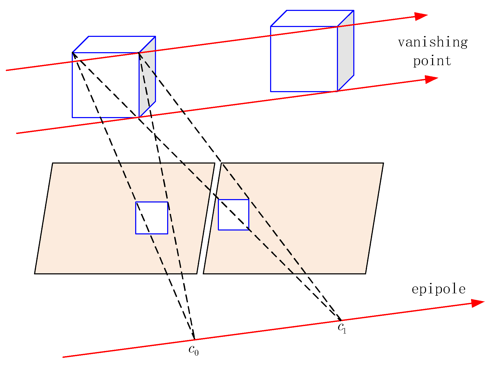
• Firstly, for the degeneracy problem caused by special positional line features during camera translation, a degeneracy phenomenon detection strategy is proposed to locate the line where the error occurs. Meanwhile, for the case of anomalous direction vectors in the Plücker coordinates, according to the coincidence between the vanishing point and epipole at infinity, the vanishing point feature is obtained to correct the vectors of the line feature and solve the degeneracy phenomenon.
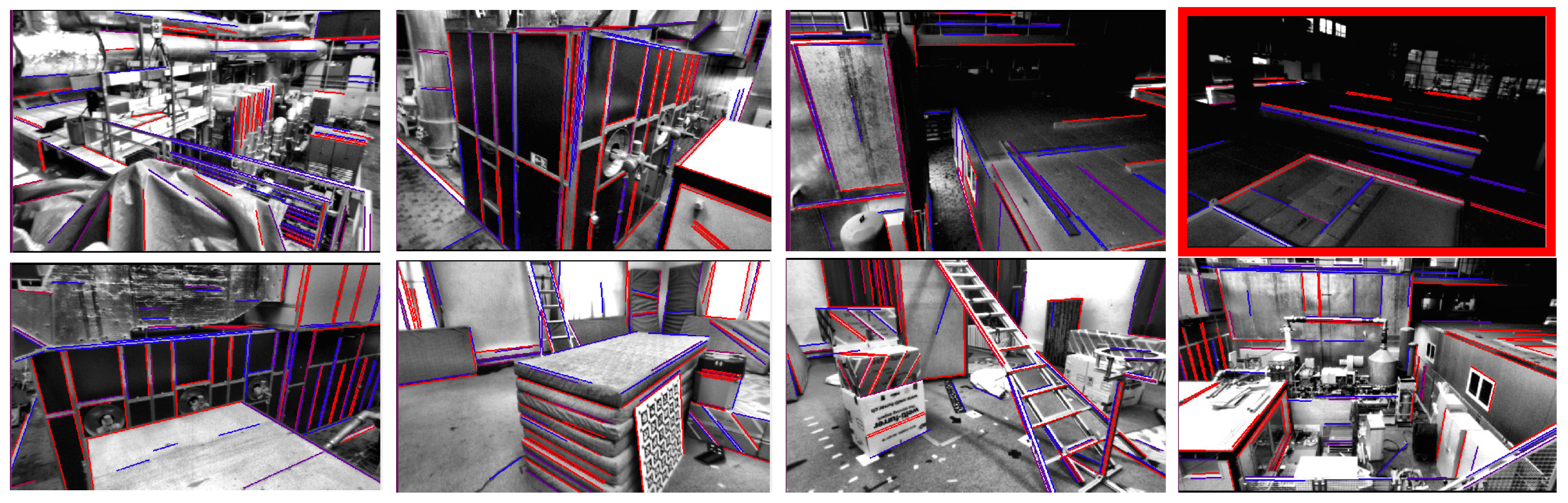
• Then, based on the characteristics of the distribution of line features in the Manhattan scene, the detected line features are categorized into structural and non-structural lines by setting length and angle threshold conditions between vanishing point and line features.
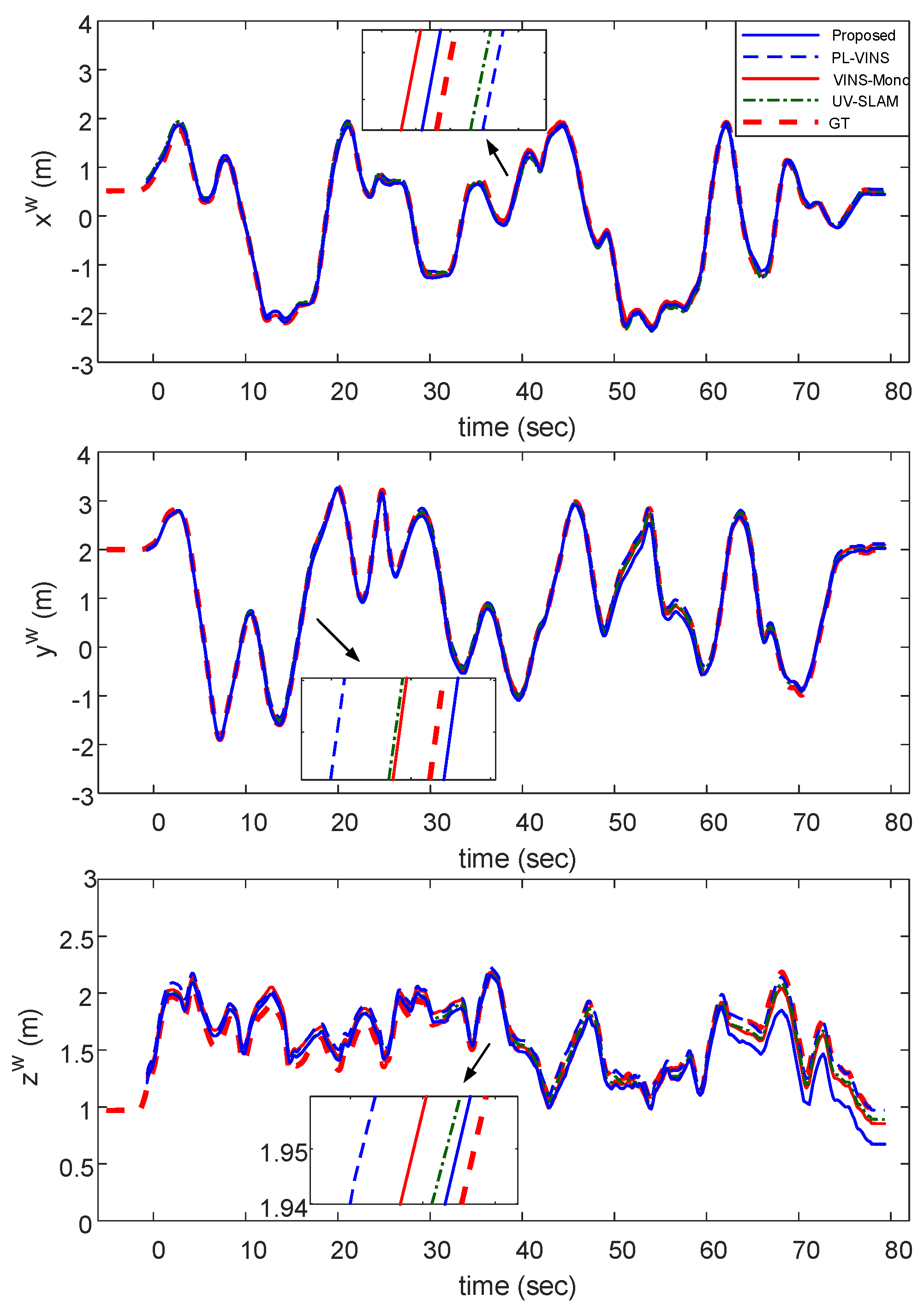
• Finally, the vanishing point residuals are added to the back-end optimization-based SLAM cost function. Experiments on two publicly available datasets validate that the proposed method improves the pose estimation and mapping accuracy of features in indoor complex environments.

2. Related Work

2.1. Line Feature Analysis

In the VIO study, line features had higher stability in harsh environments. The PL-SLAM [23] system proposed by Pumarola et al. adds a line segment detector (LSD) [24] on top of ORB-SLAM [25], which implements point feature and line feature extraction in SLAM. Fu et al. achieved real-time extraction by modifying the hidden parameters of the LSD algorithm [19]. Lee et al. fused corner point and line features to construct point-line residuals by utilizing the similarity of their positions, and the two features complemented each other to enrich the structural information of the carried environment [20]. In the above study, LSD was widely used as a line feature extractor, but it still failed to be accurate in scenarios with noise. Akinlar et al. proposed an EDLines linear timeline segment detector [26], which utilizes the edge drawing (ED) algorithm to detect edge pixels continuously, ultimately improving the detection speed while controlling the number of false detections. Liu et al. proposed a line segment extraction and merging algorithm to achieve feature tracking between points and lines with geometric constraints based on the removal of short and useless line segments [27]. Suárez et al. proposed ELSED, which utilizes a local line segment growth algorithm to align pixels by connecting gradients at breakpoints, greatly improving the efficiency of line segment detection [28]. The PLI-VINS proposed by Zhao et al. designs adaptive thresholds for line segment extraction algorithm and constructs an adjacency matrix to obtain the orientation of the line segments, which greatly improves the efficiency of the line feature processing in indoor point and line vision SLAM systems [29]. Bevilacqua et al. proposed probabilistic clustering methods using descriptors based on grid computation, which reduces the number of samples within the grid through a special pixel selection process to design new image representations for hyperspectral images [30]. The analysis of line features is summarized in

Table 1. Summary of line feature analysis.

Line Feature Analysis	Characteristics
[23]	Combining line features with point features using the LSD algorithm.
[19]	Modifying the parameters of the LSD algorithm for real-time extraction of line features.
[20]	Fusing line features and corner features using positional similarity.
[26]	Detection of line features using the ED algorithm to improve extraction speed.
[27]	An algorithm capable of extracting line features with geometric constraints is proposed.
[28]	Improving line segment detection efficiency with ELSED with a local line segment growth algorithm.
[29]	Setting an adaptive threshold algorithm for the line segment extraction process.
[30]	Proposed probabilistic clustering of line segments using descriptors based on grid computing.

.

2.2. Vanishing Points Analysis

Geometrically, a vanishing point on a spatial line is formed by intersecting the image plane with a ray parallel to the line and passing through the center of the camera [31]. Lee et al. searched for line features based on vanishing points before fusing parallel 3D straight lines and constructed parallel line residuals by removing anomalies during the clustering of multi-view lines [20]. In the camera calibration method [32] proposed by Chuang et al., multiple vanishing points are utilized to estimate the camera’s internal parameters, simplifying the calculations associated with calibration. Liu et al. proposed a two-module approach for estimating vanishing points, where the two modules are used to track clustered line features and generate a rich set of candidate points, respectively [33]. Camposec et al. detected vanishing points based on the inertial measurement and constantly updated it by the least squares method, which provided a global rotation observation around the gravity axis, thus correcting the yaw angle drift in pose estimation [34]. Li et al. projected the direction of the vanishing point of the 3D line and plane normal onto the tangent plane of the unit sphere, which estimates the rotation matrix of each image frame [35]. Li et al. involved the vanishing point in a deep multi-task learning algorithm, which was used to realize the adjustment of the camera, and then went through three sub-tasks to improve the detection accuracy of the vanishing point, and finally followed the track segmentation to determine the perimeter of the intruded area [36]. The analysis of vanishing points is summarized in

Table 2. Summary of vanishing points analysis.

Vanishing Points Analysis	Characteristics
[20]	Proposing parallel line features based on clustering of vanishing points.
[32]	Estimating the intrinsic parameters of the camera using vanishing points for camera calibration.
[33]	Proposing a two-module method for estimating vanishing points to ensure precise vanishing points for each frame’s cluster of line features.
[34]	Inertial-based measurements to detect vanishing points and continuous updating by the least squares method.
[35]	Involvement of vanishing points in deep multitask learning algorithms for camera tuning.
[36]	Projecting the vanishing point directions of 3D lines and plane normals onto the tangent plane of a unit sphere for estimating the rotation matrix.

.

2.3. Manhattan World Analysis

In the Manhattan world hypothesis, all planes in the world are aligned with three main directions, and utilizing the constraint relationship of the three axes can improve the building effect of the map and participation of line segments in SLAM. Kim et al. used structural features to estimate rotational and translational motions in RGB-D images, which were used to reduce drift during motion [37]. Li et al. first utilized a two-parameter representation of line features, using Manhattan world structure lines as features of the mapping, which not only encodes the global orientation information but also eliminates the cumulative drift of the camera [38]. StructVIO, proposed by Zou et al., uses the Atlanta world model, which contains the Manhattan world with different orientations, defines the starting frame coordinate system to represent each heading direction, and is constantly corrected by the state estimator as a state variable [39]. Lu et al. redefined the classification of line features based on the advantage that unstructured lines are not constrained by the environment and proposed frame-to-frame and frame-to-map line matching methods to initialize the two types of line segments, which significantly improved the trajectory accuracy of the system [40]. Peng et al. proposed a new Manhattan frame (MF) re-identification method based on the rotational constraints of MF-matched pairs, and a spatiotemporal consistency validation method to further optimize the global beam method parity energy function [41]. The analysis of the Manhattan world assumption is summarized in

Table 3. Summary of Manhattan world analysis.

Manhattan World Analysis	Characteristics
[37]	Utilizing structural features in RGB-D images to estimate rotational and translational motion, reducing drift during motion.
[38]	Utilizing structured lines in the Manhattan world as mapping features to encode global directional information.
[39]	Utilizing the Atlanta world model containing different Manhattan directions to define a starting frame coordinate system representing each heading direction.
[40]	Redefining the classification of line features is based on the advantage that unstructured lines are not constrained by the environment.
[41]	Proposing a new Manhattan frame re-identification method based on rotation constraints from MF match pairs, improving the accuracy of vanishing point estimation.
[36]	Projecting the vanishing point directions of 3D lines and plane normals onto the tangent plane of a unit sphere for estimating the rotation matrix.

.

3. Resolution of Degeneracy

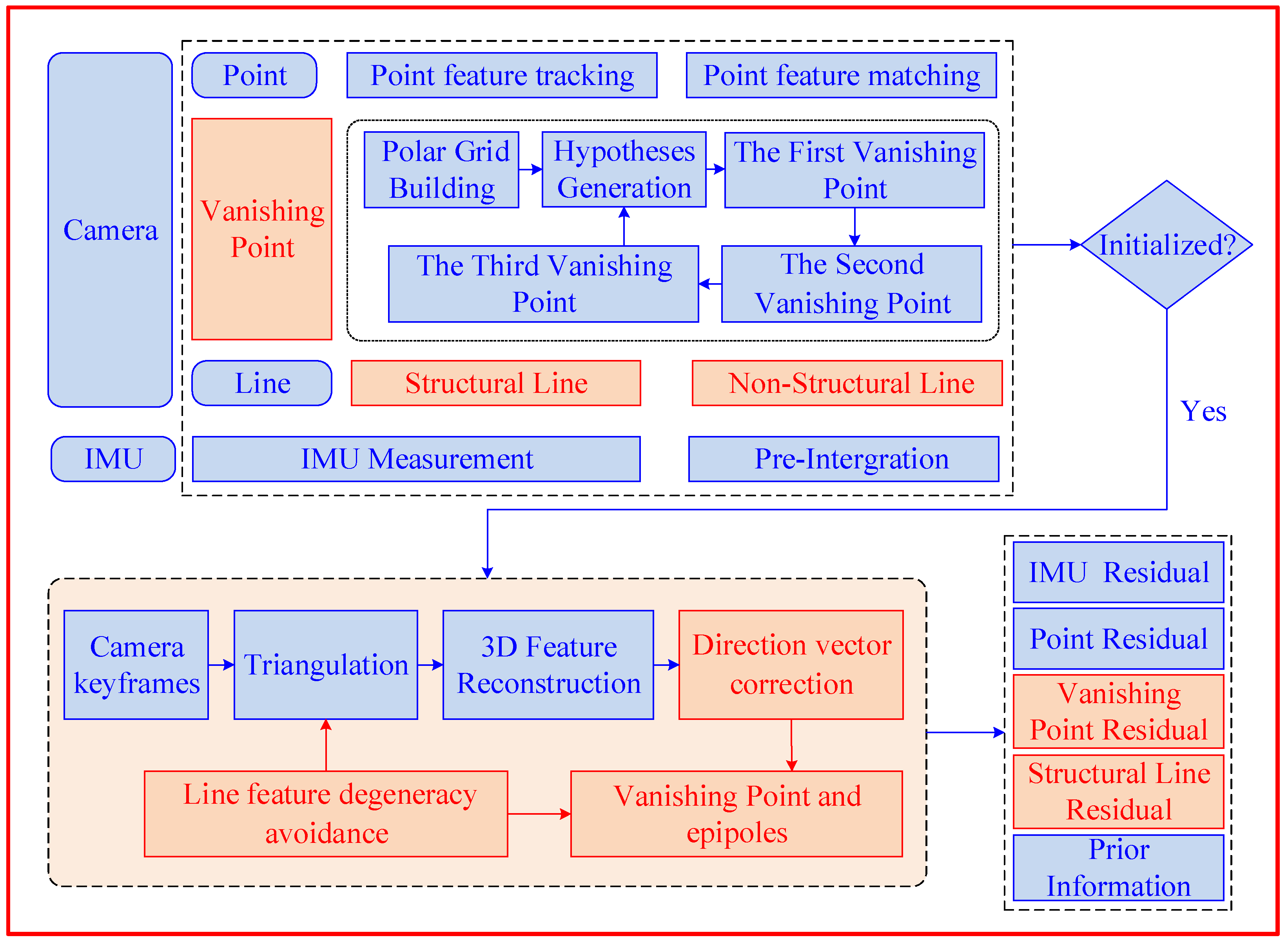
3.1. System Overview

Figure 1 shows the block diagram of the proposed visual–inertial odometer method, which fuses vanishing points and structural lines based on point features. The overall framework of the proposed method is divided into front-end and back-end data. The raw data collected by the camera and IMU were mapped onto camera frames to participate in the VIO system.

After calculating the deviation of the IMU, the pre-integration and bias correction process is performed on the IMU. Meanwhile, the points, vanishing points, and structured line features obtained from the camera are processed in parallel in the system. For the point features on the camera frames, optical flow is used for tracking and matching, and vanishing point features are filtered by RANSAC and the basic matrix model [13]. After detecting vanishing points using the two-line method [40], processing this feature is similar to point features. Following the detection of line features using the ELSED algorithm [28], structured line features meeting the criteria are identified based on Section 4.2. Keyframes are selected based on the average disparity between adjacent camera frames and the tracking quality of features, after which pose estimation of the feature and reconstruction of the environment are performed on these keyframes.

After the camera and IMU initialization phase, the system enters the triangulation stage. Degeneracy detection is applied to line features involved in epipolar constraints to calculate the position of epipoles. Then, the direction vectors of line features are corrected by incorporating vanishing points based on the relationship between vanishing points and epipoles, while features on the 2D image frames are restored to their correct positions in 3D space, as detailed in Section 3.4 and Section 3.5. Next, traditional line features are categorized into structured and unstructured lines based on vanishing point features under the Manhattan world assumption.

Finally, the line features, vanishing point features, structured line features, and prior information along with a priori information are entered into a sliding window to construct a visual–inertial bundle adjustment formulation, and the CERES solver [42] is used to compute the pose, velocities, and biases for each frame.

3.2. Representation of Line Features

In this paper, the symbols ${(·)}^w$, ${(·)}^b$, and ${(·)}^c$ represent the world coordinate system, the IMU coordinate system, and the camera coordinate system, respectively. The z-axis in the world coordinate system is aligned with the direction of gravity. In order to add line features to the monocular VIO system, the ELSED algorithm is used to detect and extract line features in images, and the LBD algorithm is used for tracking and characterization.

Point features in space can be visualized in 3D coordinates. Line features are more complex to represent compared with point features. In this paper, we use two representations of line features in PL-VIO [18], the structural lines are reconstructed using Plücker coordinates and the parameters of the line features are optimized using orthogonal coordinates. The Plücker coordinates are a six-parameter representation of the normal $n$ and direction vectors $d$ of a line feature in the Plücker coordinate system:

$$\mathcal{L}={(n^T,d^T)}^T\in R^6$$

(1)

Plücker coordinates have great advantages in the triangulation and reprojection process of line features, but they are somewhat redundant in state optimization, so a four-parameter representation of standard orthogonal coordinates is introduced:

$$\mathrm{O}=[{\psi }_1,{\psi }_2,{\psi }_3,\sigma ]$$

(2)

where ${\psi }_i$ denotes the rotation matrix of the line expressed in Euler angles in the camera coordinate system and $\sigma$ denotes the minimum distance from the center of the camera to the line. The two linear representations can be interconverted with each other by QR [43] decomposition.

3.3. Degeneracy Phenomenon Detection

In visual–inertial odometer systems with line features, degeneracy occurs during the triangulation process to recover the spatial position of features. As shown in Figure 2, when the camera is moved to a certain position, the projections $l^{\prime }$ and $l^{″}$ of the line features on two frames are located in the same line with the epipole, the planes ${\pi }_0$, ${\pi }_1$ formed by the center of the camera and projected lines coincide with the epipolar planes, and the reconstructed 3D line is located on the DABC plane:

The actual position of the line feature is at $l$, but the triangulation process may reconstruct the line feature at the position of any of the dashed lines in that plane, resulting in a biased position estimate. From the above analysis, it is clear that degeneracy occurs when the point is close to the epipole. Since there are numerous point features on line features, systems containing line features are more susceptible to degeneracy problems compared with systems with point features alone.

In response to this phenomenon, a degeneracy detection step was added to the system. Calculating the distance between the line feature and epipole can determine whether the feature is degraded or not, and the position of the epipole is calculated as follows:

$$P_{epipole}={R_{c_{i+1}}^w}^T(t_{c_i}^w-t_{c_{i+1}}^w)$$

(3)

where $P_{epipole}$ is the epipole of the $i$th camera coordinate system $c_i$ relative to the $i+1$th camera coordinate system $c_{i+1}$; $R_{c_{i+1}}^w$ is the rotation matrix from the $i+1$th camera coordinate system to the world coordinate system; and $t_{c_i}^w$ and $t_{c_{i+1}}^w$ are the translation matrices from the two camera coordinate systems to the world coordinate system, respectively.

3.4. Degeneracy Analysis

During the triangulation process, the camera coordinate systems $c_0$ and $c_1$ intersect the two planes formed by the projection lines on the two frames in a 3D straight line, forming the reconstructed spatial line. The 3D plane can be represented by a camera coordinate system and projected 2D line features:

$$\begin{array}{l}{\pi }_i=[\begin{array}{cccc}{\pi }_{ix}& {\pi }_{iy}& {\pi }_{iz}& {\pi }_{iw}\end{array}],\\ {\pi }_{ix}{c}_{ix}+{\pi }_{iy}{c}_{iy}+{\pi }_{iz}{c}_{iz}+{\pi }_{iw}=0,\\ \left[\begin{array}{c}{\pi }_{ix}\\ {\pi }_{iy}\\ {\pi }_{iz}\end{array}\right]=[s_i]\times e_i\end{array}$$

(4)

where ${\pi }_i$ is the $i$th plane vector, $s_i$ and $e_i$ are the endpoints of the tracked line segment, and their cross product can represent the value $({\pi }_{ix},{\pi }_{iy},{\pi }_{iz})$. From the equation and the camera center $c_i=(c_{ix},c_{iy},c_{iz})$ can calculate ${\pi }_{iw}$.

The direction vector of a line feature projected onto a camera frame can be calculated as follows:

$$d=\left[\begin{array}{c}{\pi }_{0z}{\pi }_{1y}-{\pi }_{0y}{\pi }_{1z}\\ {\pi }_{0x}{\pi }_{1z}-{\pi }_{0z}{\pi }_{1x}\\ {\pi }_{0y}{\pi }_{1x}-{\pi }_{0x}{\pi }_{1y}\end{array}\right]$$

(5)

As the line features approach the poles, the two plane vectors ${\pi }_0({\pi }_{0x},{\pi }_{0y},{\pi }_{0z})$ and ${\pi }_1({\pi }_{1x},{\pi }_{1y},{\pi }_{1z})$ are parallel to each other so that each element in (5) is 0 and $d$ becomes a zero matrix. In actual measurements, the estimation of the direction vectors will contain noise, which will lead to errors in the actual calculated values. Therefore, when the degeneracy phenomenon occurs, the direction vectors in Plücker coordinates will be anomalous and the mapping effect of line features will also be affected.

In the measurement model of line features, the optimized values are represented by transforming the Plücker coordinates into orthogonal coordinates. The reprojection of the line feature to the image plane can be expressed as follows:

$$l^{\prime }=\left[\begin{array}{c}{l}_1\\ l_2\\ l_3\end{array}\right]=K{n}^c$$

(6)

where $K$ represents the camera’s intrinsic parameter; $n^c$ represents the normal vector of the reprojected line feature. Since the projection plane in the optimization process is normalized and $K$ is a unit matrix, the reprojection of a spatial line is equivalent to a normal vector.

From the above analysis, it can be concluded that the degeneracy phenomenon of line features affects direction vectors in the Plücker coordinates, but the reprojection error at the back end is only related to normal vectors, so the process of solving for optimum value cannot solve the degeneracy problem.

3.5. Degeneracy Avoidance Based on Vanishing Points

In three-dimensional space, a set of parallel straight lines intersect at infinity and will be imaged under the perspective projection of the camera, and the point imaged into the two-dimensional plane is the vanishing point. So, the acquisition of a vanishing point only requires geometric analysis and does not require complex hardware equipment. Meanwhile, vanishing points can provide oriented pose information to two cameras at different positions to acquire two images of the same object, so they are often used for calibration.

Due to the specificity of the location of the vanishing point, the drift error can be reduced in pose estimation based on the feature. And the vanishing point exists on a parallel line, which does not need to be detected continuously as a point feature. Based on the above advantages, this section analyzes the connection between vanishing points and line feature degeneracy phenomena.

In the camera’s translational motion, the positions of the epipole and vanishing point on the camera frame are the same. As shown in Figure 3, the camera moves in pure translation along the x-axis, and since straight lines passing through the same point of the object are parallel, the vanishing point of the line feature is at infinity in three-dimensional space. The two camera frames are parallel to each other, and the intersection of the camera center and imaging plane is at infinity. In summary, when a line feature is projected onto a two-dimensional plane, the epipole is equivalent to a vanishing point.

By analysis, line feature degeneracy tends to occur when the camera produces pure translational motion. It can be inferred from the relationship between the spatial positions of the epipole and the vanishing point that the line features where the degeneracy phenomenon occurs have common vanishing points in the direction of the baseline.

Therefore, the problem of wrong estimation of direction vectors can be solved by introducing vanishing points based on the property that line features where the degeneracy phenomenon occurs are parallel lines. The measurement residuals of vanishing point features are:

$$r_V(z_{ij},\chi )=d_i\times d_j$$

(7)

where $d_i$ and $d_j$ represent the direction vectors of the $i$th and $j$th line features of the observation, and $\chi$ is the set of state variables.

4. Structure and Unstructured Lines

4.1. Estimation of Vanishing Points

In this paper, the two-line method is used to construct a vanishing point in Manhattan world. Firstly, a polar grid is constructed to record the response of line segments to each grid unit. Then, an equivalent spherical coordinate system centered on the camera’s focal point is defined, with the $X$ axes and $Y$ axes of the system oriented in the same direction as corresponding axes in the image plane, and the $Z$ axis pointing from the camera’s focal point to the principal point of the image.

Next, convert the coordinates of the 3D point feature in a spherical coordinate system to longitude $\lambda$ and latitude $\phi$:

$$\left\{\begin{array}{l}\phi =a\cos (Z/(X^2+Y^2+Z^2{)}^{1/2}),\\ \lambda =a\tan 2(X,Y)+\pi .\end{array}\right.$$

(8)

where $X$ and $Y$ are obtained by differencing the horizontal and vertical coordinates of pixel ${(x,y)}^T$ and principal point ${(x_0,y_0)}^T$, and $Z$ is the focal length.

For each pair of line segments $l_1$ and $l_2$ in the image plane, record their intersection $v_1$ as the first vanishing point, and compute longitude and latitude values of $v_1$ based on the coordinate transformation relationship.

Then, the cumulative equation is used to update the response of line pairs on the polar grid to achieve a greater weighting of line segments with longer lengths and moderate directional deviations:

$$p({\varphi }_i,{\lambda }_i)=p({\varphi }_i,{\lambda }_i)+‖l_1‖\times ‖l_2‖\times \sin (2\theta )$$

(9)

where ${\varphi }_i$ and ${\lambda }_i$ denote the unit values of the corresponding degrees of $\phi$ and $\lambda$, respectively. $‖l_1‖$ and $‖l_2‖$ represent lengths of the two-line segments and $\theta$ is defined as angular difference between the two segments.

According to the orthogonal constraint of the two points, the second vanishing point $v_2$ lies on the great circle of the plane formed by $v_1$ and the center of projection. The circle is sampled uniformly into 360 equal parts, with each unit corresponding to the longitude of a hypothetical vanishing point, and $v_2$ can be determined by finding the value of longitude that satisfies orthogonality with $v_1$:

$$\left\{\begin{array}{c}{X}_2=\sin (\varphi )\times \sin (\lambda )\\ \begin{array}{l}{Y}_2=\sin (\varphi )\times \cos (\lambda )\\ Z_2=\cos (\varphi )\end{array}\end{array}\right.$$

(10)

where $X_2,Y_2$, and $Z_2$ are the coordinates of $v_2$.

After calculating the first vanishing point $v_1$ and the second vanishing point $v_2$, the third vanishing point is obtained according to the constraint relation $v_3=v_1\times v_2$.

4.2. Classification of Structured and Unstructured Lines

The scene in the Manhattan World hypothesis consists of vertical and horizontal surfaces, and most of the intersecting lines of building surfaces are aligned with the three directions, $xyz$. Therefore, straight lines can be recognized as structural lines aligned with the three axes of the Manhattan world based on vanishing points in the image, and the rest of the line segments are categorized as non-structural lines.

After finding a vanishing point in space, its location can be calculated based on three dominant directions of the Manhattan world. The $x$ axis is calculated as follows:

$$v_x^{{\psi }_i}=K{R}_w^c{[\cos {\psi }_i,-\sin {\psi }_i,0]}^T$$

(11)

where ${\psi }_i\in [0,\pi /2),(i=1,2,\dots ,N)$ denotes the heading of the localized Manhattan world, and $R_w^c$ is the rotation matrix from the world coordinate system to the camera coordinate system. Similarly, the vanishing point in the $y$ axis direction is:

$$v_y^{{\psi }_i}=K{R}_w^c{[\sin {\psi }_i,\cos {\psi }_i,0]}^T$$

(12)

The vanishing point in the $z$ axis direction is independent of the heading of the Manhattan world, which is calculated as:

$$v_z=K{R}_w^c{[0,0,1]}^T$$

(13)

The theoretical location of the vanishing point in relation to the structure line is as follows:

$$\left\{\begin{array}{c}\tau (v_1) · L_1=0\\ \tau (v_2) · L_2=0\\ \tau (v_3) · L_3=0\end{array}\right.$$

(14)

where $\tau$ represents the transformation from camera coordinates to image coordinates, and $L_1,L_2,L_3$ represents the structure line with the direction of the vanishing point.

In this paper, the threshold detection method is used to judge the direction of structural lines. First, a ray is drawn from the vanishing point to the midpoint position of the line feature. Then, a distance threshold $d_t$ and an angle threshold ${\theta }_t$ are set to categorize the line feature into three directions. Specifically, if the distance from the vanishing point to the midpoint is less than $d_t$ and the angle to the line feature is less than ${\theta }_t$, the line feature is considered a structural line in the corresponding direction. If more than one vanishing point satisfies the line feature detection condition, the one with the best consistency is selected and the corresponding local Manhattan world is constructed on the basis of that vanishing point.

Line segments that do not meet the threshold are appended to a similar Manhattan world based on angle and distance, and when the number of proximally categorized line features is greater than 50% of the total number of detected lines, the detection of vanishing points in all three directions is continued using the two-line method, which further identifies the line features to new Manhattan worlds based on the threshold. Finally, unclassified line features are recognized as unstructured lines.

4.3. Back-End Optimization

In the vanishing point measurement model, the vanishing points corresponding to line features are added as new measurements in the optimization process of the sliding window:

$$v^c=\left[\begin{array}{c}{v}_1\\ v_2\\ v_3\end{array}\right]={\lim }_{t\to \infty }PV(t)=K{d}^c$$

(15)

where $V(t)$ is the homogeneous coordinate of the vanishing point, $t\in (0,\infty )$ is a parameter in the coordinate representation, and $P=K\left[\mathrm{I}|0\right]$ is the internal reference matrix of the camera. It follows from (15) that the vanishing points on the line features are equivalent to the direction vectors on the line.

The intersection of the observation model of the vanishing point and image plane is regarded as the measurement of the vanishing point feature. As shown in Figure 4, the recovered spatial line without degeneracy is the red solid line $l_e$, but the actual line is the blue solid line $l_r$, and the projections of the two lines on the normalized plane are the dashed lines of the corresponding colors, respectively. The intersections $v_e$ and $v_r$ between the two dashed lines and projection plane are the estimated value and observed value of the vanishing point, where the coordinate of $v_e$ is $(v_1/v_3,v_2/v_3,1)$. The residuals at vanishing point $r_v$ are defined as:

$$r_v=\frac{1}{v_3}\left[\begin{array}{c}{v}_1\\ v_2\end{array}\right]-v_r$$

(16)

The Jacobi matrix associated with the vanishing point is:

$$J_v=\frac{\partial r_v}{\partial v^c}\frac{\partial v^c}{\partial L^c}\left[\begin{array}{cc}\frac{\partial L^c}{\partial \delta x}& \frac{\partial L^c}{\partial L^w}\frac{\partial L^w}{\delta \mathcal{O}}\end{array}\right]$$

(17)

where $\delta x$ and $\delta \mathcal{O}$ are state variables of the IMU and the structural line. Each part of (17) is specified as:

$$\begin{array}{l}\frac{\partial r_v}{\partial v^c}=\left[\begin{array}{ccc}-\frac{1}{v_3}& 0& \frac{v_1}{{v_3}^2}\\ 0& -\frac{1}{v_3}& \frac{v_2}{{v_3}^2}\end{array}\right],\\ \frac{\partial v^c}{\partial L^c}=\left[\begin{array}{cc}{0}_{3\times 3}& K_{3\times 3}\end{array}\right]=\left[\begin{array}{cc}{0}_{3\times 3}& I_{3\times 3}\end{array}\right]\end{array}$$

(18)

where $I$ is the unit matrix.

After obtaining state estimates for each variable, joint optimization is performed in a sliding window:

$$\begin{array}{l}\chi =[x_0,x_1,\cdots ,x_m,{\lambda }_0,{\lambda }_1,\cdots {\lambda }_n,0_0,0_1,\cdots 0_k],\\ x_i=[p_{b_i}^w,q_{b_i}^w,v_{b_i}^w,b_a,b_g],\\ 0_k=[{\psi }_k,{\sigma }_k].\end{array}$$

(19)

where $x_i$ denotes a state of the IMU in the $i$th sliding window, specifically including the position of the IMU in the world coordinate system, the quaternion, the velocity, and the bias of the accelerometer and gyroscope. The ${\lambda }_n$ in the overall state variable represents the inverse depth of the point feature in the sliding window from the first observation. $0_k$ denotes the first structural line feature orthogonalized in the world coordinate system. $m,n,k$ denotes the number of keyframes, point features, and structural line features in the optimization process, respectively.

5. Experimental Validation

In this section, experiments were performed on an Intel Core i7-11800H processor (Intel, Santa Clara, CA, USA) with 16GB RAM and an Ubuntu 16.04LTS system. In order to evaluate the performance of the proposed method, this paper tested 11 datasets from the EuRoC micro aerial vehicle (MAV) datasets [44] and 7 datasets from the TUM VI Benchmark dataset [45].

The proposed method is based on the VINS-Mono and UV-SLAM methods in this paper. The VINS-Mono, PL-VINS, and UV-SLAM methods were each run five times under the same configuration environment and dataset as comparison data, where VINS uses only point features and PL-VINS uses point and line features. Both UV-SLAM and the proposed method use point, structured line, and vanishing point features, with the proposed method adding unstructured line features. Throughout the tests, the default parameters provided by the authors were used and loopback detection was turned off to test only the odometer performance.

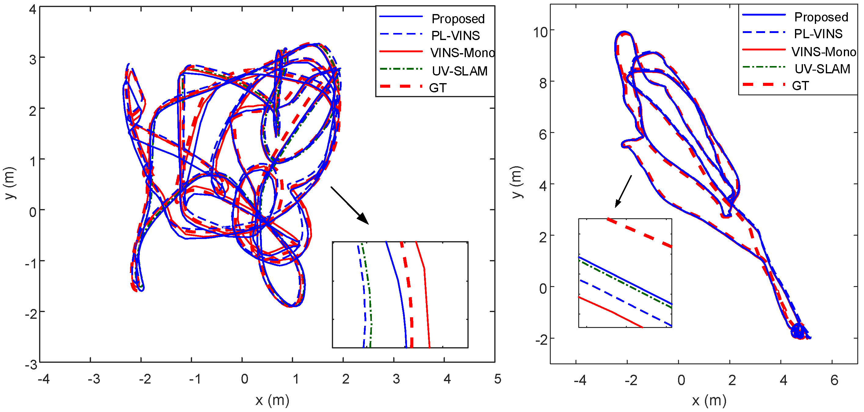
5.1. EuroC MAV Dataset

The EuRoC Micro Aerial Vehicle (MAV) dataset was collected by a quadcopter in three different environments, including the machine hall and the VICON room. In experiments of this paper, only the left camera image frames were used for pose estimation. Figure 5 shows the experimental snapshots of the proposed method under 11 sequences. From the figure, it can be seen that the proposed method still has good robustness in low-illumination environments. The root mean square error (RMSE) of the absolute trajectory error was used to evaluate localization accuracy, while the average RMSE of each VIO system was calculated to demonstrate performance improvement. The RMSE values of VINS-Mono, PL-VINS, UV-SLAM, and the proposed method for 11 sequences are shown in

Table 4. RMSE APE (meter) of VINS-MONO, PL-VINS, UV-SLAM, and the proposed method.

Experiment	VINS-Mono	PL-VINS	UV-SLAM	Proposed
MH_01_easy	0.230	0.234	0.212	0.200
MH_02_easy	0.164	0.160	0.154	0.148
MH_03_medium	0.251	0.250	0.247	0.238
MH_04_difficult	0.462	0.358	0.356	0.351
MH_05_difficult	0.334	0.326	0.325	0.313
V1_01_easy	0.085	0.083	0.078	0.078
V1_02_medium	0.142	0.165	0.106	0.096
V1_03_difficult	0.184	0.178	0.174	0.167
V2_01_easy	0.097	0.098	0.091	0.086
V2_02_medium	0.266	0.111	0.114	0.112
V2_03_difficult	0.328	0.351	0.334	0.333
Average	0.231	0.201	0.199	0.193
Enhance	19.07%	8.35%	2.88%	—

, with the values denoted in bold black being closest to the true value.

Localization errors were evaluated by the root mean square error from the Evo package (https://github.com/MichaelGrupp/evo) and two-dimensional pose trajectories were evaluated by the MATLAB 2018a_win64 software package. The MH scene is narrower and full of texture, and the theoretical case works better under the point feature system VINS-Mono, but according to Table 4, the proposed method shows superiority in all five sequences. The VICON scene motion blur is prone to degradation, and the proposed algorithm introduces structural and non-structural line constraints to reduce the mapping error compared with the PL-VINS.

Figure 6 provides an evolution of localization results of the proposed method in three directions $xyz$ under V1_02_medium. As can be seen from the figure, the localization results improve significantly with time. Figure 7 shows the trajectory maps of MH_02_easy and V1_02_medium sequences in the plane. It can be seen that in most scenarios, the proposed method obtains the trajectory estimation closest to the true value in the comparison experiments.

Figure 8 demonstrates the comparison plot of pose trajectory error between UV-SLAM and the proposed method on MH_03_medium, V1_03_ difficult, and V2_01_easy sequences, where the redder color of the trajectory represents the larger error. From the above results, it is clear that the proposed method has a smaller error compared with other methods.

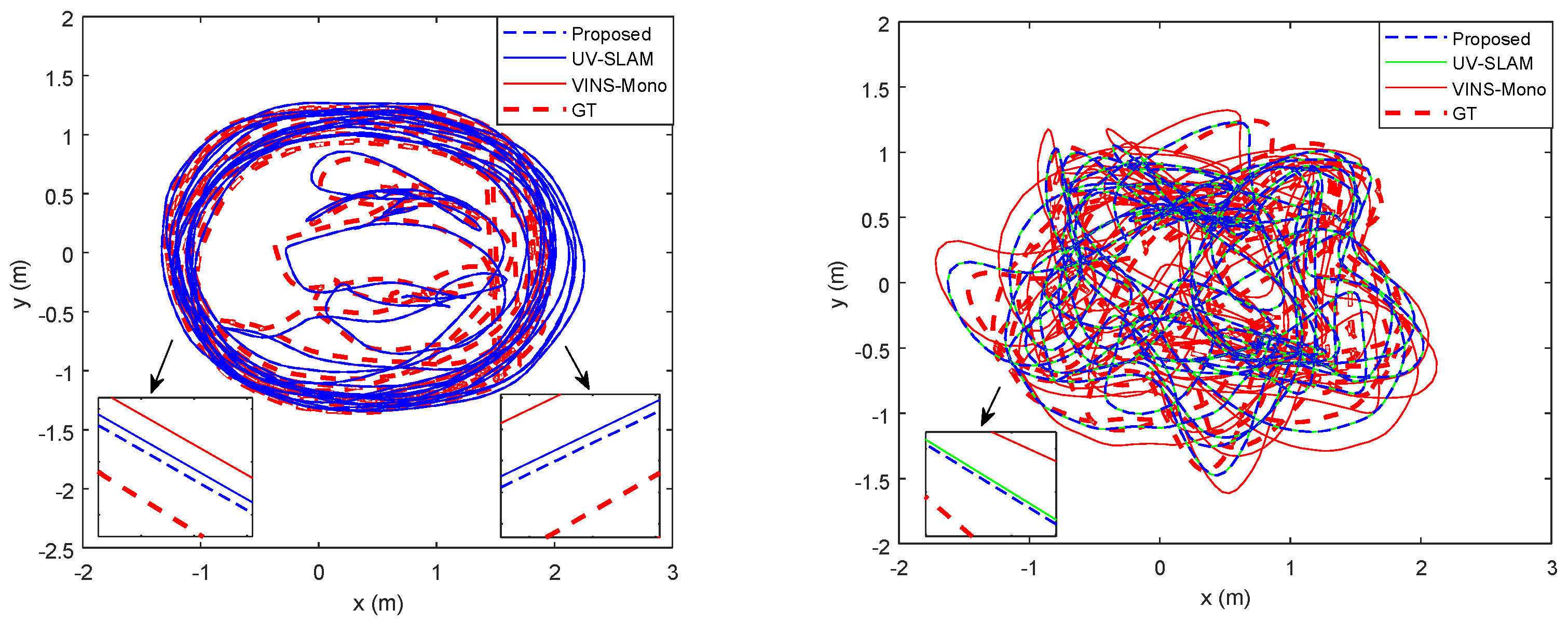
5.2. TUM-VI Benchmark Dataset

The TUM-VI Benchmark dataset was captured by a handheld fisheye stereo Kinect camera, which contains hallway, lobby, outdoor, indoor, and slide scenes. The entirety of the room sequence carries a true value of motion capture and the background of the proposed method is an indoor environment, so the room1 to room6 sequences were selected for testing in this experiment. The complexity of the scene is also increased by selecting the slide1 sequence of the slide scene, for which the state estimates are computed from the truth values of the start and end phases.

In the section, the proposed method was compared with VINS-Mono and UV-SLAM. The ATE values of each algorithm were calculated separately as shown in

Table 5. RMSE APE (meter) of VINS-MONO, UV-SLAM, and the proposed method on the TUM-VI Benchmark dataset.

Experiment	VINS-Mono	UV-SLAM	Proposed
room1_512_16	0.094	0.079	0.071 1
room2_512_16	0.069	0.068	0.067
room3_512_16	0.248	0.127	0.121
room4_512_16	0.041	0.042	0.042
room5_512_16	0.340	0.216	0.210
room6_512_16	0.071	0.069	0.070
slide1_512_16	0.583	0.495	0.426
Average	0.206	0.157	0.144
Enhance	42.80%	8.65%	—

¹ Values in bold indicate the closest true value.

. UV-SLAM utilizes both point and structured line features, but due to the lack of unstructured line constraints in the irregular Manhattan scene, the algorithm induces a large directional drift with an average RMSE of 0.157. As can be seen from the comparison results in Table 5, the proposed method achieves the minimum translation error, and the trajectory accuracy is improved by 42.80% and 8.65%, respectively.

Figure 9 plots the local detail comparison trajectories for room2 and room5 where the three systems are able to extract a maximum of 150 point features and 30 line features from the input image frame. The narrow and violently rotating indoor sequence scene poses a greater challenge to the stability of the algorithm, but the figure visualizes that the two sequences have less fluctuation and lower cumulative drift compared with the two representative VIO systems, VINS-Mono and UV-SLAM.

Figure 10 shows the APE evolution plots of VINS-Mono proposed on room1_512_16, room3_512_16, and room5_512_16 sequences with respect to Table 2. Each set of experiments has a smaller error result for the proposed method. From the above results, it can be concluded that the proposed method effectively improves the performance of motion estimation.

6. Conclusions

A new visual–inertial odometry method is proposed based on vanishing point features with structured and unstructured line constraints in indoor environments. The method considers the line feature degeneracy phenomenon that occurs during the feature-matching stage, and the degeneracy detection condition is designed to compute the position of the epipole in order to identify the line where the degradation problem occurs. By analyzing the optimization variables in the reprojection phase, the property in which the vanishing point coincides with the epipole at infinity is exploited for degeneracy avoidance as well as for optimization of the direction vectors in Plücker coordinates. At the same time, the threshold condition is set to classify the line features into structural and non-structural lines in order to enhance the richness of line features in 3D scenes. Finally, point, structural line, and vanishing point features are jointly added to the state estimation process for sliding window optimization. By comparing the results with the classical VIO methods on two public datasets, it was verified that the proposed method effectively improves the accuracy and robustness of state estimation.

References

1. Jeon, J.; Jung, S.; Lee, E.; Choi, D.; Myung, H. Run your visual-inertial odometry on NVIDIA jetson: Benchmark tests on a micro aerial vehicle. IEEE Robot. Autom. Lett. 2021, 6, 5332–5339. [Google Scholar] [CrossRef]
2. Campos, C.; Elvira, R. ORB-SLAM3: An accurate open-source library for visual, visual-inertial, and Multi-map SLAM. IEEE Trans. Robot. 2021, 37, 1874–1890. [Google Scholar] [CrossRef]
3. Yang, N.; Stumberg, L.; Wang, R.; Cremers, D. D3VO: Deep depth, deep pose and deep uncertainty for monocular visual odometry. In Proceedings of the IEEE/CVF Conference on Computer Vision and Pattern Recognition (CVPR), Seattle, WA, USA, 13–19 June 2020. [Google Scholar]
4. Teng, Z.; Han, B.; Cao, J.; Hao, Q.; Tang, X.; Li, Z. PLI-SLAM: A Tightly-Coupled Stereo Visual-Inertial SLAM System with Point and Line Features. Appl. Sci. 2023, 15, 4678. [Google Scholar] [CrossRef]
5. Zhang, Y.; Huang, Y.; Zhang, Z.; Postolache, O.; Mi, C. A vision-based container position measuring system for ARMG. Meas. Control 2023, 56, 596–605. [Google Scholar] [CrossRef]
6. Duan, H.; Xin, L.; Xu, Y.; Zhao, G.; Chen, S. Eagle-vision-inspired visual measurement algorithm for UAV’s autonomous landing. Int. J. Robot. Autom. 2020, 35, 94–100. [Google Scholar] [CrossRef]
7. Usenko, V.; Demmel, N.; Schubert, D.; Stückler, J.; Cremers, D. Visual inertial mapping with non-linear factor recovery. IEEE Robot. Autom. Lett. 2020, 5, 422–429. [Google Scholar] [CrossRef]
8. Forster, C.; Pizzoli, M.; Scaramuzza, D. SVO: Fast semi-direct monocular visual odometry. In Proceedings of the IEEE International Conference on Robotics and Automation (ICRA), Hong Kong, China, 31 May–7 June 2014. [Google Scholar]
9. Engel, J.; Koltun, V.; Cremers, D. Direct sparse odometry. IEEE Trans. Pattern Anal. Mach. Intell. 2018, 40, 611–625. [Google Scholar] [CrossRef] [PubMed]
10. Shen, S.; Michael, N.; Kumar, V. Tightly-coupled monocular visual-inertial fusion for autonomous flight of rotorcraft MAVs. In Proceedings of the IEEE International Conference on Robotics and Automation (ICRA), Seattle, WA, USA, 26–30 May 2015. [Google Scholar]
11. Li, M.; Mourikis, A. High-precision, consistent EKF-based visual inertial odometry. Int. J. Robot. Res. 2013, 32, 690–711. [Google Scholar] [CrossRef]
12. Bloesch, M.; Burri, M.; Omari, S.; Hutter, M.; Siegwart, R. Iterated extended kalman filter based visual-inertial odometry using direct photometric feedback. Int. J. Robot. Res. 2017, 36, 1053–1072. [Google Scholar] [CrossRef]
13. Qin, T.; Li, P.; Shen, S. VINS-Mono: A robust and versatile monocular visual-inertial state estimator. IEEE Trans. Robot. 2018, 34, 1004–1020. [Google Scholar] [CrossRef]
14. Leutenegger, S.; Lynen, S.; Bosse, M.; Siegwart, R.; Furgale, P. Keyframe-based visual-inertial odometry using nonlinear optimization. Int. J. Robot. Res. 2014, 34, 314–334. [Google Scholar] [CrossRef]
15. Greene, W.; Roy, N. Metrically-scaled monocular slam using learned scale factors. In Proceedings of the IEEE International Conference on Robotics and Automation (ICRA), Paris, France, 31 May–31 August 2020. [Google Scholar]
16. Cui, H.; Tu, D.; Tang, F.; Xu, P.; Liu, H.; Shen, S. Vidsfm: Robust and accurate structure-from-motion for monocular videos. IEEE Trans. Image Proc. 2022, 31, 2449–2462. [Google Scholar] [CrossRef] [PubMed]
17. Lee, S.; Hwang, S. Elaborate monocular point and line slam with robust initialization. In Proceedings of the IEEE/CVF International Conference on Computer Vision (ICCV), Seoul, Republic of Korea, 27 October–2 November 2019. [Google Scholar]
18. He, Y.; Zhao, J.; Guo, Y.; He, W.; Yuan, K. Pl-VIO: Tightly-coupled monocular visual–inertial odometry using point and line features. Sensors 2018, 18, 1159. [Google Scholar] [CrossRef] [PubMed]
19. Fu, Q.; Wang, J.; Yu, H.; Ali, I.; Guo, F.; He, Y.; Zhang, H. PL-VINS: Real-time monocular visual-inertial SLAM with point and line features. arXiv 2020, arXiv:2009.07462. [Google Scholar]
20. Lee, J.; Park, S. PLF-VINS: Real-time monocular visual-inertial SLAM with point-line fusion and parallel-line fusion. IEEE Robot. Autom. Lett. 2021, 6, 7033–7040. [Google Scholar] [CrossRef]
21. Gomez-Ojeda, R.; Briales, J.; Gonzalez-Jimenez, J. PL-SVO: Semi-direct monocular visual odometry by combining points and line segments. In Proceedings of the IEEE/RSJ International Conference on Intelligent Robots and Systems (IROS), Daejeon, Republic of Korea, 9–14 October 2016. [Google Scholar]
22. Lim, H.; Jeon, J.; Myung, H. UV-SLAM: Unconstrained line-based SLAM using vanishing points for structural mapping. IEEE Robot. Autom. Lett. 2022, 7, 1518–1525. [Google Scholar] [CrossRef]
23. Pumarola, A.; Vakhitov, A.; Agudo, A.; Sanfeliu, A.; Moreno-Noguer, F. PL-SLAM: Real-time monocular visual SLAM with points and lines. In Proceedings of the IEEE International Conference on Robotics and Automation (ICRA), Singapore, 29 May–3 June 2017. [Google Scholar]
24. Von Gioi, R.; Jakubowicz, J.; Morel, J.; Randall, G. LSD: A fast line segment detector with a false detection control. IEEE Trans. Pattern Anal. Mach. Intell. 2010, 32, 722–732. [Google Scholar] [CrossRef] [PubMed]
25. Mur-Artal, R.; Tardós, J. ORB-SLAM2: An open-source slam system for monocular, stereo, and RGB-D cameras. IEEE Trans. Robot. 2017, 33, 1255–1262. [Google Scholar] [CrossRef]
26. Akinlar, C.; Topal, C. EDLines: A real-time line segment detector with a false detection control. Patt. Recog. Lett. 2011, 32, 1633–1642. [Google Scholar] [CrossRef]
27. Liu, Z.; Shi, D.; Li, R.; Qin, W.; Zhang, Y.; Ren, X. PLC-VIO: Visual-Inertial Odometry Based on Point-Line Constraints. IEEE Trans. Autom. Sci. Eng. 2021, 19, 1880–1897. [Google Scholar] [CrossRef]
28. Suárez, I.; Buenaposada, J.; Baumela, L. ELSED: Enhanced line SEgment drawing. arXiv 2022, arXiv:2108.03144. [Google Scholar] [CrossRef]
29. Zhao, Z.; Song, T.; Xing, B.; Lei, Y.; Wang, Z. PLI-VINS: Visual-Inertial SLAM based on point-line feature fusion in Indoor Environment. Sensors 2022, 22, 5457. [Google Scholar] [CrossRef]
30. Bevilacqua, M.; Berthoumieu, Y. Multiple-feature kernel-based probabilistic clustering for unsupervised band selection. IEEE Trans. Geosci. Remote Sens. 2019, 57, 6675–6689. [Google Scholar] [CrossRef]
31. Cipolla, R.; Drummond, T.; Robertson, D. Camera Calibration from Vanishing Points in Image of Architectural Scenes. In Proceedings of the British Machine Vision Conference 1999, Nottingham, UK, 13–16 September 1999; Volume 38, pp. 382–391. [Google Scholar]
32. Chuang, J.; Ho, C.; Umam, A.; Chen, H.; Hwang, J.; Chen, T. Geometry-based camera calibration using closed-form solution of principal line. IEEE Trans. Image Process. 2021, 30, 2599–2610. [Google Scholar] [CrossRef] [PubMed]
33. Liu, J.; Meng, Z. Visual SLAM with drift-free rotation estimation in manhattan world. IEEE Robot. Autom. Lett. 2020, 5, 6512–6519. [Google Scholar] [CrossRef]
34. Camposeco, F.; Pollefeys, M. Using vanishing points to improve visual-inertial odometry. In Proceedings of the IEEE International Conference on Robotics and Automation (ICRA), Seattle, WA, USA, 26–30 May 2015. [Google Scholar]
35. Li, Y.; Yunus, R.; Brasch, N.; Navab, N.; Tombari, F. RGB-D SLAM with structural regularities. In Proceedings of the IEEE International Conference on Robotics and Automation (ICRA), Xi’an, China, 30 May–5 June 2021. [Google Scholar]
36. Li, X.; Zhu, L.; Yu, Z.; Guo, B.; Wan, Y. Vanishing Point Detection and Rail Segmentation Based on Deep Multi-Task Learning. IEEE Access 2020, 8, 163015–163025. [Google Scholar] [CrossRef]
37. Kim, P.; Coltin, B.; Kim, H. Low-drift visual odometry in structured environments by decoupling rotational and translational motion. In Proceedings of the IEEE International Conference on Robotics and Automation (ICRA), Brisbane, Australia, 21–25 May 2018. [Google Scholar]
38. Li, Y.; Brasch, N.; Wang, Y.; Navab, N.; Tombari, F. Structure-SLAM: Low-drift monocular SLAM in indoor environments. IEEE Robot. Autom. Lett. 2020, 5, 6583–6590. [Google Scholar] [CrossRef]
39. Zou, D.; Wu, Y.; Pei, L.; Ling, H.; Yu, W. StructVIO: Visual-inertial odometry with structural regularity of man-made environments. IEEE Trans. Robot. 2019, 35, 999–1013. [Google Scholar] [CrossRef]
40. Lu, X.; Yao, J.; Li, H.; Liu, Y.; Zhang, X. 2-line exhaustive searching for real-time vanishing point estimation in manhattan world. In Proceedings of the IEEE Winter Conference on Applications of Computer Vision (WACV), Santa Rosa, CA, USA, 24–31 March 2017. [Google Scholar]
41. Peng, X.; Liu, Z.; Wang, Q.; Kim, Y.; Lee, H. Accurate visual-inertial slam by manhattan frame re-identification. In Proceedings of the IEEE/RSJ International Conference on Intelligent Robots and Systems (IROS), Prague, Czech Republic, 27 September–1 October 2021. [Google Scholar]
42. Agarwal, S.; Mierle, K. Ceres Solver. Available online: http://ceres-solver.org (accessed on 9 April 2018).
43. Bartoli, A.; Sturm, P. Structure-from-motion using lines: Representation, triangulation, and bundle adjustment. Comput. Vis. Image Underst. 2005, 100, 416–441. [Google Scholar] [CrossRef]
44. Burri, M.; Nikolic, J.; Siegwart, R. The EuRoC micro aerial vehicle datasets. Int. J. Robot. Res. 2016, 35, 1157–1163. [Google Scholar] [CrossRef]
45. Schubert, D.; Goll, T.; Demmel, T.; Usenko, V.; Stückler, J.; Cremers, D. The TUM VI benchmark for evaluating visual-inertial odometry. In Proceedings of the IEEE/RSJ International Conference on Intelligent Robots and Systems (IROS), Madrid, Spain, 1–5 October 2018. [Google Scholar]
Figure 1. Block diagram for the proposed method.
Applsci 14 01990 g001
Figure 2. Illustrative diagram of degeneracy phenomenon of line features.
Applsci 14 01990 g002
Figure 3. Analytical diagram of the relationship between spatial positions of the vanishing point and the epipole.
Applsci 14 01990 g003
Figure 4. Schematic diagram of the residuals at vanishing point.
Applsci 14 01990 g004
Figure 5. The experiment snapshots of the EuRoC dataset by the proposed method.
Applsci 14 01990 g005
Figure 6. Evolution of localization with respect to the V1_02_medium sequence (blue solid lines: the proposed method; blue dashed lines: PL−VINS; green solid lines: UV−SLAM; red solid lines: VINS−Mono; and red thick dashed lines: ground truth).
Applsci 14 01990 g006
Figure 7. Comparative paths with respect to V1_02_medium (left) and MH_02_easy (right) (blue solid lines: the proposed method; blue dashed lines: PL−VINS; green solid lines: UV−SLAM; red solid lines: VINS−Mono; and red thick dashed lines: ground truth).
Applsci 14 01990 g007
Figure 8. Comparison of the pose trajectory error of UV-SLAM (left) and the proposed method (right) (top plots: MH_03_medium; middle plots: V1_03_ difficult; bottom plots: V2_01_easy; left: UV-SLAM; and right: the proposed method).
Applsci 14 01990 g008
Figure 9. Comparative paths with respect to room2_512_16 (left) and room5_512_16 (right) (blue dashed lines: the proposed method; green solid lines: UV−SLAM; red solid lines: VINS−Mono; and red thick dashed lines: ground truth).
Applsci 14 01990 g009
Figure 10. APE evolution results regarding VINS-Mono (left) and the proposed method (right) experiments (top plots: room1_512_16; middle plots: room3_512_16; and bottom plots: room5_512_16).
Applsci 14 01990 g010