Performance Evaluation of L₁-Norm-Based Blind Deconvolution after Noise Reduction with Non-Subsampled Contourlet Transform in Light Microscopy Images

Abstract

Noise and blurring in light microscope images are representative factors that affect accurate identification of cellular and subcellular structures in biological research. In this study, a method for l₁-norm-based blind deconvolution after noise reduction with non-subsampled contourlet transform (NSCT) was designed and applied to a light microscope image to analyze its feasibility. The designed NSCT-based algorithm first separated the low- and high-frequency components. Then, the restored microscope image and the deblurred and denoised images were compared and evaluated. In both the simulations and experiments, the average coefficient of variation (COV) value in the image using the proposed NSCT-based algorithm showed similar values compared to the denoised image; moreover, it significantly improved the results compared with that of the degraded image. In particular, we confirmed that the restored image in the experiment improved the COV by approximately 2.52 times compared with the deblurred image, and the NSCT-based proposed algorithm showed the best performance in both the peak signal-to-noise ratio and edge preservation index in the simulation. In conclusion, the proposed algorithm was successfully modeled, and the applicability of the proposed method in light microscope images was proved based on various quantitative evaluation indices.

1. Introduction

A microscope allows researchers to visualize and study the structures and functions of specimens at a cellular and subcellular level. It is a device that combines an optical lens and a mechanical device and comprises a system that can achieve high magnification. Among the types of microscopes, light microscope is the most basic and is configured to directly observe the light passing through the specimen.

Light microscope images often appear blurry because light from one point on the sample is not detected in a single pixel. This is caused by the fundamental limitation that light from a very small point cannot be detected from a similar point. Therefore, light can be detected only in a small area when the image is in focus [1]. In a non-ideal case, the obtained image is convolved with a point spread function (PSF) that provides the imaging system response with a degraded resolution. In particular, blurring should be removed through pre-calibration by considering the theoretical resolution and cross sectional capacity of the imaging system [2]. However, there is a limit to completely removing the PSF. Therefore, PSF estimation and deconvolution to the image acquisition condition are essential for high-quality restoration [3].

Deblurring approaches are divided into non-blind deblurring (performs deconvolution by knowing the PSF in advance) and blind deblurring (estimates the PSF and performs deconvolution without relying on ancillary measurements). Non-blind deblurring methods have previously been investigated using various approaches, including the image-formation model [4,5], inverse filtering [6], Tihkonov regularization [7], Landweber [8], fast iterative soft-thresholding [9], Richardson-Lucy [10,11,12], and maximum a posteriori method [13]. The corresponding representative algorithms are described in detail in the literature [1,14]. Unfortunately, these methods depend on a prior PSF that is based on the laws of optics using the theory and knowledge of the optical components, and the PSF is unlikely to match the current experimental conditions [1].

Accurate PSF estimation is the key to successful image restoration in blind deblurring. Typical blind deblurring methods include parametric form-based methods [15,16], joint image restoration and blur identification methods [17,18], Bayesian-based methods [19,20], prior-knowledge-based methods [21,22], and the adaptive image deconvolution algorithm [13,23]. Various studies have shown that these methods effectively estimate the PSF and exhibit outstanding image restoration results, even in ill-posed problems. However, the presence of noise in the microscope image is still a problem.

The degraded image can be modeled by convolving a clean image, which is artifact free, and the blur kernel (or PSF) of a light microscope imaging system, as follows:

$$g\left(x,y\right)=f\left(x,y\right)⨂⨂psf\left(x,y\right)+n\left(x,y\right),$$

(1)

where g(x,y) and f(x,y) are degraded and clean images, respectively; psf(x,y) represents the blur kernel; and n(x,y) is the added background noise. The noise that can be generated in an optical microscopic image includes Poisson noise from the number of photons, Gaussian noise from image sensor and ambient noise, quantization noise from the analog-to-digital conversion, and speckle noise from coherent light sources [24]. Image restoration based on a model that comprehensively considers various noises will produce accurate results. However, it is not feasible to implement a degradation model takes all noise components. Among the various noise degradation models, the additive noise model of the Gaussian distribution, which is universally assumed by transmitted-light microscopy, was selected in this study. For instance, Willis et al. [25] assumed that white Gaussian noise was added to the original image (artifact free) in the process of performing 3D image reconstruction in transmitted light bright-field microscopy, and Theodore et al. [26] modeled and conducted research in the form of adding Gaussian noise while simulating the light intensity curve of charge-coupled device (CCD)-based light microscopy. In addition, previous studies for noise reduction [27,28,29] have investigated that the degrading process of conventional microscopy system using photomultiplier, CCD, and complementary metal-oxide-semiconductor sensors can be described as Equation (1), and this study performed based on this assumption. The presence of noise in the image leads to challenges in the accurate estimation of PSF and noise amplification owing to similar high-pass filtering. In addition, noise reduction introduces additional blurring by low-pass filtering, which affects the intrinsic PSF of the light microscopy imaging system. Thus, it is different from the intrinsic PSF.

Proposed method improves the resolution preventing the noise amplification based on the multi-resolution analysis (MRA) and noise level prediction for each subband image in light microscopy image. In addition, we also restored the blur components generated by the system and noise reduction algorithms with a blind deconvolution method to improve the resolution. This approach can derive improvement in sharpness while preventing image deterioration due to noise amplification shown in other state-of-the-art methods, thereby improving overall image quality. Blind deconvolution method is the most reasonable approach to predicting the final PSF. Blind deconvolution attempts to estimate the final PSF, without relying on auxiliary measures. It is to resort to iteratively until minimization of fidelity term in object function. This is a very challenging nonlinear problem [14]. Among image restoration techniques, MRA has been representatively used because it can effectively separate several frequency components while considering the spatial domain [30,31]. Recently, convolution neural network denoiser and regularized term-based iterative method was presented to restore the noise and sharpness [32]. Moreover, deep learning module based on U-Net and half instance normalization block was introduced and this showed the outstanding results in terms of visual perception and evaluation metrics [33].

We investigated l₁-norm-based blind deconvolution after noise reduction with a non-subsampled contourlet transform (NSCT) [34] in light microscopic images and evaluated the image performance. First, we describe the proposed restoration scheme using light microscope images, materials and conditions for the simulation and experiment, and factors for a quantitative evaluation. Then, we present and analyze the results and demonstrate the effectiveness of the proposed framework on both the simulated and experimentally acquired data. Finally, based on the results and subsequent discussion, the main conclusions of this study are summarized.

2. Materials and Methods

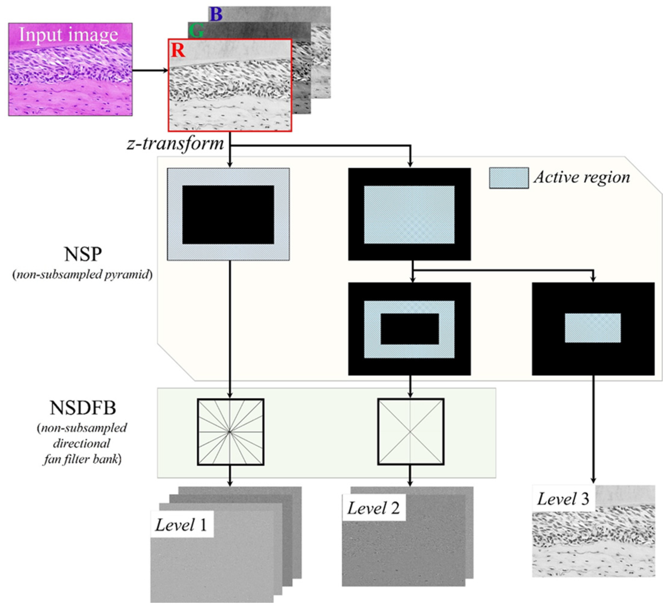
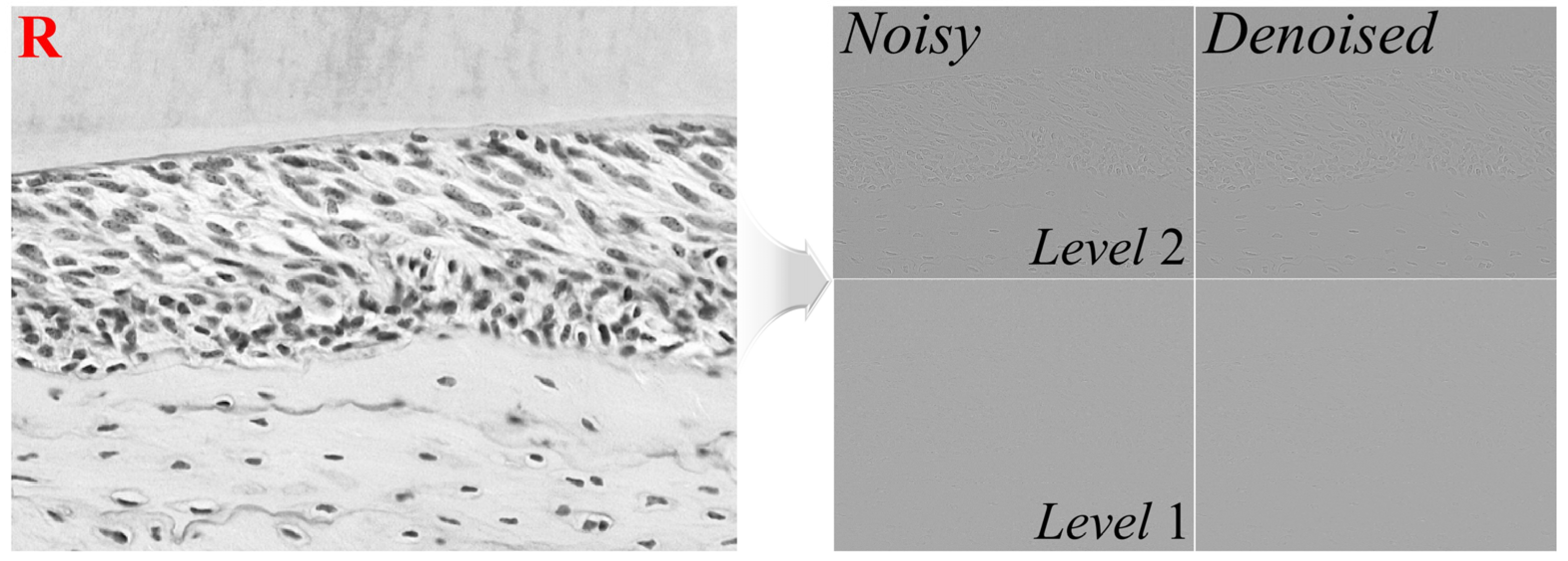
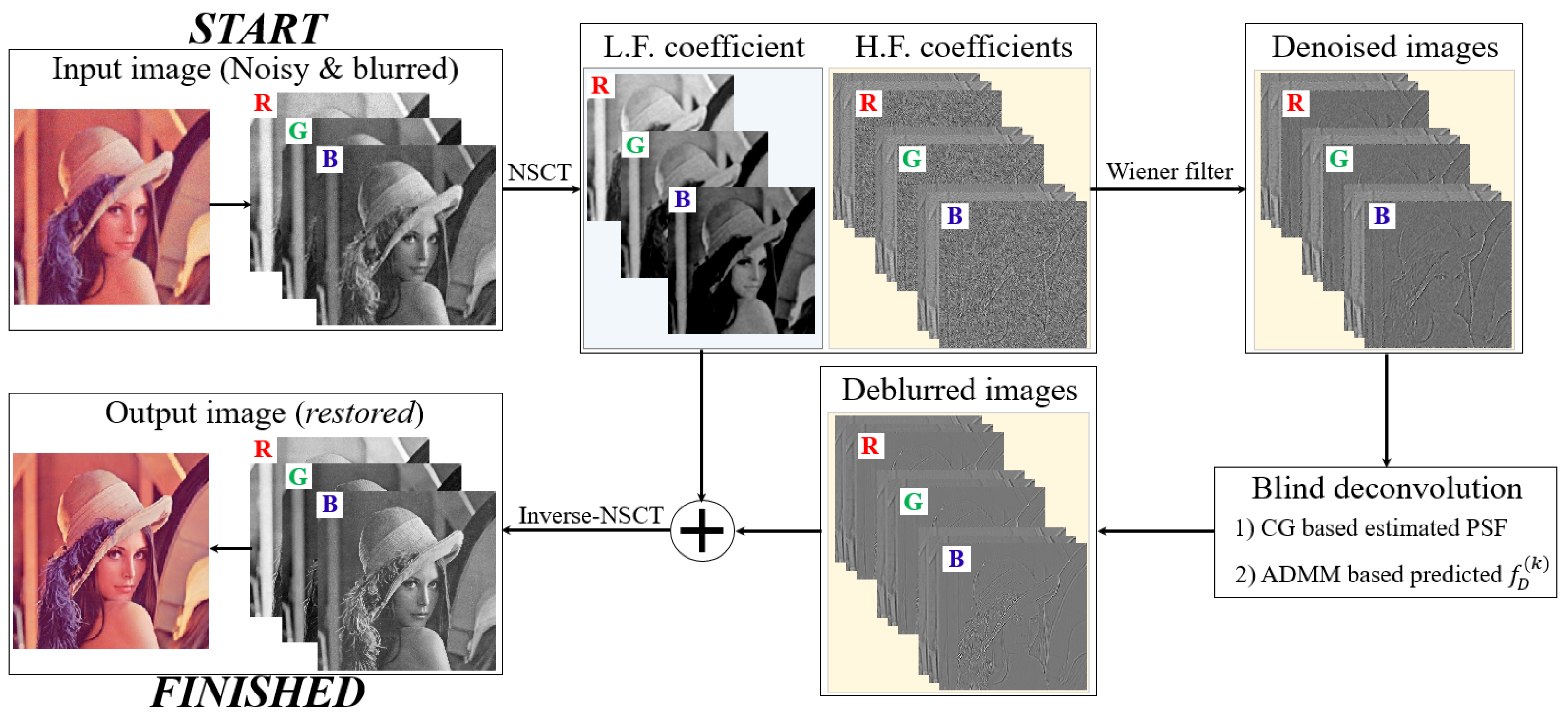
2.1. Proposed Restoration Scheme for Microscopic Images

Do and Vetterli [35] introduced the contourlet transform (CT), which is divided into flexible multiscale and multidirectional expansions. However, it has a limitation—the shift-invariance property is unfulfilled while performing up- and downsampling. NSCT overcomes this problem. Figure 1 shows a simplified NSCT flowchart for a microscopic image. The NSCT decomposition process is classified into two phases: (1) non-subsampled pyramid (NSP) and (2) non-subsampled directional fan filter bank (NSDFB). The NSP separates the low- and high-frequency subband images while maintaining the shift-invariant relationship, and then decomposes the high-frequency subband images at each level [36]. Subsequently, the NSCT can be reconstructed without data loss to ensure the shift-invariant property and detect detailed features according to direction. More information is available in the literature [37].

We implemented noise reduction in a suitable frequency region via NSCT. Figure 2 shows some of examples; noisy and denoising image among the high-frequency subbands images of R-channel degraded image using NSCT. Wiener filtering [38] was used to reduce the noise component. By using the NSCT, we can obtain a successful noise reduction by assigning appropriate parameters of the denoising algorithm in each image, which are divided according to frequency and filter direction. Here, we used the 2D modified Wiener filtering (MMWF) method to reduce the noise component. MMWF has advantage of mean and Wiener filtering in terms of maintaining resolution, even though noise reduction has been implemented [39] and it can be written in Equation (2)

$$MMWF\left(x,y\right)=\widetilde{g_{\mathsf{\Omega }}}+\frac{{\sigma }_{\mathsf{\Omega }}^2-n_{\mathsf{\Omega }}^2}{{\sigma }_{\mathsf{\Omega }}^2}(g_{\mathsf{\Omega }}\left(x,y\right)-\widetilde{g_{\mathsf{\Omega }}}),$$

(2)

where $\widetilde{g_{\mathsf{\Omega }}}$ and ${\sigma }_{\mathsf{\Omega }}$ are the mean value and standard deviation in mask $\mathsf{\Omega }$, respectively, and $n_{\mathsf{\Omega }}$ is the standard variation of noise. We investigated the size of $\mathsf{\Omega }$ according to the Ju et al. [40] and empirically set to 11 $\times$ 11 pixels in simulation and experiment. In addition, $n_{\mathsf{\Omega }}$ was calculated by finding the accurate noise level using the homogeous blocks. The previous studies [41,42,43] introduce structure-oriented noise estimation the method that eight directional high-pass filters were applied to the microscopy image and then the resulting image was added. The 10% of pixels with the smallest sum were selected. This is assumed to be a homogeneous block containing only noise. This method has the advantage of effectively extracting homogeneous block, but the disadvantage is that the process of selecting homogeneous block reflects human error, making it difficult to produce consistent results. Sutour et al. [44], has introduced an effective method to estimate the noise parameters. The input image was divided into small blocks and the homogenous block selected (e.g., 10 $\times$ 10 pixels, empirically). Here, the homogeonous blocks are an assumption that noise variation is the dominant factor. Sutour’s paper indicates that the larger the block size, the better the accuracy in predicting the noise level. However, within the proposed image size, a larger block size means fewer blocks extracted. Sutour’s study used a block of 16 $\times$ 16 pixels in 512 $\times$ 512 pixels in optical image. Applying these conditions to our experiments, we extracted fewer than 30 homogeneous blocks on average, despite the much larger image size (3264 $\times$ 2448 pixels). Through trial and error, we selected a block size of 10 $\times$ 10 pixels that reliably predicted the noise level in each NSCT domain. Note that the block size chosen is not absolute, as it can change depending on the conditions of the light microscopy imaging system. This block can detection used the rank correlation such as kendall’s $\tau$-coefficient method [45,46]. It can select the homogeous block with high similarity by correlating them in four-directional expanded kendall’s $\tau$-coefficient. The noise level can be calculated by averaging the standard deviation of the selected blocks and $n_{\mathsf{\Omega }}^2$ was used as the predicted noise level each subband images. Thus, there is an advantage in obtaining an optimal noise removal effect while preserving the un-sharpness compared to performing noise reduction on a single image.

After reducing the effect on noise, each high-frequency component was performed using the blind deconvolution scheme to restore the blur artifact resulting from the finite focal spot size and denoising process. First, we used the conjugate gradient-based framework to estimate the PSF between the Laplacian image of ${f_D}^{\left(k\right)}$ and g, according to Kim et al. [47]:

$${\nabla }^{2}g\left(x,y\right)={\nabla }^2{f_D}^{\left(k\right)}\left(x,y\right)⨂⨂{psf}^{\left(k\right)}\left(x,y\right),$$

(3)

where ${\nabla }^2$ is the Laplacian operator. Here, differential image was acquired to extract only the edge information. Then, ${f_D}^{(k+1)}$ is predicted to solve the object function using the l₁-norm-based regularization term as follows:

$${f_D}^{(k+1)}\left(x,y\right)=\underset{f^{\left(k\right)}\in Q}{\mathrm{argmin}}\frac{\alpha }{2}{‖{f_D}^{\left(k\right)}\left(x,y\right)⨂⨂{psf}^{\left(k+1\right)}\left(x,y\right)-g(x,y)‖}_2^2+{‖\nabla {f_D}^{\left(k\right)}\left(x,y\right)‖}_1,$$

(4)

where Q is the set of feasible values of ${f_D}^{\left(k\right)}$ and $\alpha$ is a parameter that balances the two terms. When matches between the edge information of the degraded image and that of blurred image by convolving the appropriate PSF in clean image, the PSF can be considered as the optimal PSF of the optical microscope imaging system, and the process of repeating Equations (3) and (4) are performed to satisfy this requirement. Chan et al., investigated the performance of proposed algorithm in total variation (TV)/l₁ problem [48]. When using an objective function to obtain a deblurred image from a noisy image, it was difficult to give much weight to the regularization term due to increase the possibility of obtained the smoothing results. To overcome this limitation, our previous study demonstrated that proposed approach by setting the regularization term based on weight map and l₁-norm improved the sharpness of image without cartoonish artifact [49]. The l₀-norm-based deconvolution method without weight function was applied to the deblurred image for improving the resolution. In addition, we optimized the balance parameter values between the fidelity and regularization terms through trial and error until the discrepancy between the current and updated results converged to 10⁻⁶. Therefore, $\alpha$ is chosen such that the signal-to-noise ratio is maximized (In this study, $\alpha =500$ was empirically used in the experiment). Finally, the optimization problem is calculated through the alternating direction method of multipliers (ADMM) method to find the optimal solution. This method is discussed in detail in a previous work [48].

Figure 3 shows the proposed restoration scheme flowchart incorporating the l₁-norm-based blind deconvolution and NSCT in light microscopy images. Briefly, a degraded image is acquired from the light microscope system (①), low- and high-frequency coefficients are separated via NSCT, and noise reduction is performed with the appropriate parameter considering each high-frequency coefficient (②). Subsequently, the deblurred images (③), which are calculated by entering the blind deconvolution scheme to improve the sharpness, are inversely transformed with the existing low-frequency coefficient (④). Here, the same process was performed on all channels, and the impact of the process on the channel is independent. Finally, the restored image is acquired (⑤).

2.2. Materials and Conditions for the Simulation and Experiment

In simulation, the used Lena image was of size 512 $\times$ 512 pixels and three-dimensional (3D) (i.e., width, height, and depth (3-color channel)). A simulation study was performed using Lena images to evaluate prior possibilities before applying the proposed algorithm to real light microscopy images. Here, the image was properly selected to perform the simulation because of its well-matched detail, shadow, and texture, which is good for handling the proposed algorithm. Figure 4 shows the blurred PSF (${\sigma }_{PSF}$ = 1, arbitrarily unit) plot and Gaussian noise image (mean = 0 and variance = 0.01) to generate the degraded image, as shown in Equation (1). Noise generation was performed using imnoise function (MATLABTM, R2021a, Mathworks, Natick, MA, USA). These values are different from the image degradation that occurs when acquiring light microscopy images in our experiments. However, they are arbitrarily assigned to perform a quantitative performance evaluation of the proposed algorithm and are sufficient for the original purpose of performing the simulation.

In experiment, microscopy images were obtained using a Leica DM500 microscope and Leica ICC50 E camera (Leica Microsystem, Wetzlar, Germany, readout noise (σ) < 6 least-significant bit, typical), and Leica LAS EZ 3.0 software (Leica Microsystem, Wetzlar, Germany). In this work, we aim to derive optimal PSF and to restore the intrinsic resolution of optical microscopy system. ICR male mice (Orientbio, Seongnam, Republic of Korea) were used to obtain the light microscopic images. The mandibles were dissected from the mice and immediately fixed in 4% paraformaldehyde (PFA) at 4 °C for 24 h. For decalcification, the samples were treated with 10% ethylenediaminetetraacetic acid (EDTA) for four weeks. The specimens were dehydrated and embedded in paraffin. They were cut to a thickness of 7-μm and stained with hematoxylin and eosin (H&E) routinely used for histological examination. Histological images including the bone, periodontal ligament (PDL), and tooth of mandible were taken under the light microscope. Exposure times ranged from 2 ms to 600 s, and implemented the gain, offset, and shading correction. Numerical aperture (NA) value is 0.280, field of depth at dry objective is about 8 μm, 400× magnification is used in this study.

Based on the above descriptions, we implemented the proposed algorithm using computing environment: CPU: Intel, Santa Clara, CA, USA, Xeon Platinum 8168 @ 2.70 GHz; RAM: Samsung, Suwon, Republic of Korea, 8 G × 4 DDR4 21,300; GPU: NVIDIA, Santa Clara, CA, USA, GTX 1080 11 GB. The acquired microscopy image is in tiff format and composed of 3-channel data, which were derived by applying the proposed algorithm to the obtained images in the wavelet domain. The processing time of proposed algorithm in 512 × 512 pixels image is approximately less than 2 s with the GPU parallel processing, which confirms the utility for practical applications.

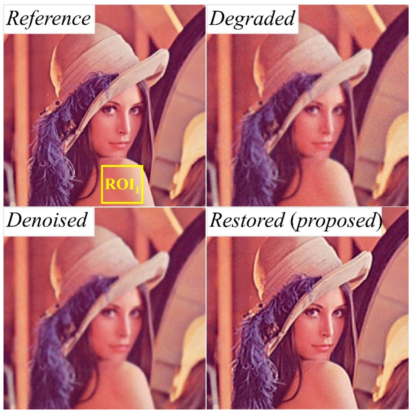
2.3. Quantitative Image Quality Evaluation

The quantitative performance of the designed scheme for light microscopy images was evaluated in terms of visual assessment, coefficient of variation (COV), peak signal-to-noise ratio (PSNR), and edge preservation index (EPI) [50], which are defined as:

$$COV=\frac{S_I}{M_I},$$

(5)

$$\begin{gathered} SNR=20{log}_{10}\left({MAX}_I\right)-10{log}_{10}\left(MSE\right) \mathrm{and} \\ MSE=\frac{1}{mn}{\sum }_{i=0}^{m-1}{\sum }_{j=0}^{n-1}{[R\left(i,j\right)-I(i,j\left)\right]}^2, \end{gathered}$$

(6)

$$\begin{gathered} EPI=\frac{\mathsf{\Gamma }\left(⊿p_1-\overline{\mathsf{⊿}{p}_1},\mathsf{⊿}{p}_2-\overline{\mathsf{⊿}{p}_2}\right)}{\sqrt{\left(\mathsf{⊿}{p}_1-\overline{\mathsf{⊿}{p}_1},\mathsf{⊿}{p}_1-\overline{\mathsf{⊿}{p}_1}\right)}\circ \mathsf{\Gamma }\left(\mathsf{⊿}{p}_2-\overline{\mathsf{⊿}{p}_2},\mathsf{⊿}{p}_2-\overline{\mathsf{⊿}{p}_2}\right)} \mathrm{and} \\ \mathsf{\Gamma }\left(a,b\right)={{\sum }_{i,j\in ROI}a\left(i,j\right)b\left(i,j\right)}^2, \end{gathered}$$

(7)

where $S_I$ and $M_I$ are the mean and standard deviation of the input image, respectively; ${MAX}_I$ is the maximum value of the input data; $R\left(i,j\right)$ is the reference value of $\left(i,j\right)$ index without in the reference image of the m$\times$n matrix; $p_1$ and $p_2$ are the reference and measured data, respectively; and $\overline{\mathsf{⊿}p}$ is the implementation of Laplacian filtering in the region of interest (ROI). The ROI for evaluating COV was set based on the distribution of the simplest tissues.

To evaluate the usefulness of the proposed algorithm for the blurring effect that appears when focusing on a desired point in each of the three areas, no-reference-based evaluation parameters were used. The no-reference-based evaluation parameters used in this study were the natural image quality evaluator (NIQE) [51] and blind/referenceless image spatial quality evaluator (BRISQUE) [52], which are commonly applied in the imaging field. BRISQUE and NIQE evaluate image quality based on generalized Gaussian distribution (GGD) and multivariate Gaussian (MVG) fitting, respectively, and are expressed as follows [51,52]:

$${\mathrm{f}}_{GGD}\left(x;a,{\sigma }^2\right)=\frac{\alpha }{2\beta ∆\left(\raisebox{1ex}{$1$}\!\left/ \!\raisebox{-1ex}{$\alpha $}\right.\right)}exp\left(-{\left(\frac{\left|x\right|}{\beta }\right)}^{\alpha }\right),$$

(8)

$${\mathrm{D}}_{MVG}\left(v_1,v_2,{\mathsf{\Sigma }}_1,{\mathsf{\Sigma }}_2\right)=\sqrt{\left({\left(v_1-v_2\right)}^T{\left(\frac{{\mathsf{\Sigma }}_1+{\mathsf{\Sigma }}_2}{2}\right)}^{-1}\left(v_1-v_2\right)\right)},$$

(9)

where $a$ denotes the shape parameter that controls the distribution of ${\sigma }^2$; $∆$ is the gamma function; $\beta$ = $\sigma \sqrt{\frac{∆\left(\raisebox{1ex}{$1$}\!\left/ \!\raisebox{-1ex}{$\alpha $}\right.\right)}{∆\left(\raisebox{1ex}{$3$}\!\left/ \!\raisebox{-1ex}{$\alpha $}\right.\right)}}$; $v_1$ and ${\mathsf{\Sigma }}_1$ denote the vector and covariance matrices of an ideal image, respectively; and $v_2$ and ${\mathsf{\Sigma }}_2$ denote the vector and covariance matrices of the test image, respectively.

The gradient magnitude (GM) calculated the magnitude of the slope of image and it determines variation of edges [53]. It can be expressed as follows:

$$GM\left(i\right)=\sqrt{{\left(J⨂f_h\right)}^2\left(i\right)+{\left(J⨂f_v\right)}^2\left(i\right)},$$

(10)

where $J$ is microscopy image, $f_h$ and $f_v$ are 3 $\times$ 3 template gradient filter yields the horizontal and vertical direction, and ⨂ operator used the convolution between $J$ and gradient filter. The high value of gradient magnitude indicates that the sharpness has relatively higher.

Quantitative evaluation was performed using a total of 20 light microscopic images, and the average value was derived.

3. Results and Discussion

Figure 5 shows examples of the reference image (left top), degraded image (right top), denoised image (left bottom) from the degraded image, and restored (proposed) image (right bottom) using the proposed NSCT-based multiresolution analysis. The restored (proposed) image result exhibits a superior image quality with regard to sharpness and noise level compared to those of the degraded and denoised images.

Figure 6 shows the quantitative evaluation results for the COV, PSNR, and EPI metrics of the simulated Lena images. To separately analyze the colors of the three channels observed in the acquired image, the quantitative evaluation results and average values for red (R), green (G), and blue (B) were derived. In all the quantitative evaluation results, the R, G, and B data showed similar trends. The COV results increased in the following order: reference, denoised, restored, and degraded images (Figure 6a). The average COV values of the restored image obtained using the proposed NSCT algorithm and the denoised image were approximately 0.237 and 0.180, respectively. When the proposed NSCT algorithm was applied to the obtained Lena image, the COV deteriorated by approximately 1.31 times compared to the image with noise reduction alone. However, we confirmed that the COV of the image after applying the proposed algorithm improved by approximately 2.44 times compared to the degraded image without image processing. The analyzed PSNR values were lowest in the degraded image and highest in the restored image (Figure 6b). The average PSNR values of the restored image obtained with the proposed NSCT algorithm and the denoised image were approximately 38.71 and 27.98, respectively. When the proposed NSCT algorithm was applied to the obtained Lena image, we confirmed that the PSNR improved by 1.44 and 1.38 times compared with the degraded and denoised images, respectively. The evaluated EPI values were the highest in the restored image and lowest in the denoised image (Figure 6c). The average EPI values of the restored image obtained using the proposed NSCT algorithm and degraded image were approximately 0.758 and 0.573, respectively. When the proposed NSCT algorithm was applied to the obtained Lena image, we confirmed that the EPI results were improved by 1.32 and 1.58 times compared to the degraded and denoised images, respectively. These results for the simulated Lena image indicate that the proposed NSCT algorithm is useful in terms of noise improvement and edge region preservation. Referring to Figure 6a, for COV, which can evaluate the ratio of noise and signal simultaneously, the best result can only be derived from the denoised image, except for the reference Lena image. However, the part in which the COV result improved by approximately 2.44 times compared to the degraded image in the Lena image after applying the NSCT algorithm means that the denoising performance of the proposed method is within an achievable range. In particular, the best result was obtained from the image to which the NSCT algorithm was applied in terms of the PSNR evaluation result, which shows the degree of image quality loss as the maximum value of the input data and the mean square error (Figure 6b). This means that the NSCT algorithm has excellent overall image restoration performance. In addition, EPI, which indicates the degree of image edge preservation, showed the best value when using the NSCT algorithm, similar to the PSNR result (Figure 6c). Note that, the COV value can be high not only when the noise is removed, but also when the edge component is smoothing. In the case of Figure 6a, the COV value of the restored image is expected to be higher than that of the denoised image due to increase the variation of signal during the deconvolution process. On the other hand, the EPI factor of the restored image is larger than that of the denoised image, which may be occurred due to over smoothing during the denoising process. Moreover, the sharpness of the degraded image is lower than that of the reference image. It is almost same effect as blurring when performing Laplacian filtering when the contours contain the noise component in image. It will be led to the low EPI value. Based on a comprehensive analysis of the PSNR, COV, and EPI results, we deduce that the restored image using the proposed method achieves the appropriate balance between the noise reduction and sharpness preservation. In addition, by performing a quantitative evaluation for each image restoration method in the simulated Lena image, we demonstrated that the proposed NSCT algorithm can effectively preserve the image edge information and simultaneously reduce the noise level efficiently.

Figure 7a shows the difference images compared to the reference image of degraded image (left), denoised image (middle), and restored image (right) and these enlarged images. The error of difference image between the restored image and the reference image is significantly less than that of other images, qualitatively. Moreover, Figure 7b shows the histogram bar graph and MSE results of them. The histogram plot of the difference image between restored image and reference image trends to be lower than that of other images, and MSE results of the difference image of restored image are about 1.27 and 1.02 times lower, compared to that of other images. These results indicated that the restored image using the proposed method accurately removed the noise and blurring components from the degraded image so that the restored image is close to the reference image.

Figure 8a shows the results of applying the image quality improvement methods to the light microscopy image of the mandible tissue of mouse. The acquired light microscopy images consisted of the tooth, PDL, and bone tissue from top to bottom and the enlarged images for arrow areas in Figure 8a are shown in Figure 8b–d. From the visual evaluation of the resulting image, it was confirmed that the sharpness of the deblurred image was improved compared with that of the degraded image in all areas of the tooth, PDL, and bone. Here, the deblurred image was generated by applying the previously l₀-norm-based blind deconvolution method [49] to compare the results of the proposed method. Noise amplification in the deblurred image occurred significantly in all areas, and the noise level of the image could be reduced using the denoising method. However, there were cell types in the PDL tissue that were not well observed in the denoised image; we were able to overcome this disadvantage by using the proposed NSCT algorithm (Figure 8c).

Figure 9 shows the quantitative evaluation results for the light microscopic images of the mandible tissue of male mice in terms of the COV. The COV result graph was calculated for ROI₁ in Figure 8a. Similar to the simulation analysis, the COV was analyzed by dividing the R, G, and B colors by the channel in the real light microscopic image. Consequently, the highest and lowest COV values were derived for the deblurred and denoised images, respectively. The average COV values of the restored experimental image obtained using the proposed NSCT algorithm and the denoised experimental image were approximately 0.496 and 0.259, respectively. In particular, we demonstrated that the COV result for the restored image improved by approximately 2.52 times compared to that of the deblurred image.

Even in the experimental results, the COV of the denoised image was more improved than that of the restored image; however, a no-reference-based evaluation method was used to analyze the image quality considering the overall sharpness. Figure 10 shows the quantitative evaluation results for the no-reference-based evaluation parameters, including NIQE and BRISQUE, of the light microscopy images of the mandible tissue of real male mice. For the deblurred, denoised, and restored images, the obtained NIQE results yielded values of 3.52, 5.20, and 3.88 for the deblurred, denoised, and restored images, respectively. Compared to the denoised image, we confirmed that the NIQE result for the restored image improved by approximately 1.34 times. In addition, the obtained BRISQUE results yielded values of 16.09, 38.57, and 20.08 for the deblurred, denoised, and restored images, respectively. Compared with the denoised image, we confirmed that the BRISQUE result for the restored image improved by approximately 1.92 times.

As it is difficult to quantitatively evaluate the spatial resolution in a real experimental image, the NIQE and BRISQUE parameters were used to evaluate the overall image quality without using a reference. In the two no-reference-based evaluation results, it was demonstrated that the restored image can properly reduce noise and blurring in the light microscopic image compared to the denoised image. In the COV result, which can quantitatively evaluate the noise level, a superior value was shown in the denoised image; however, edge information was lost owing to excessive blurring in the acquired image. In addition, the NIQE and BRISQUE results based on natural scene statistics exhibited similar tendencies, confirming the usefulness of the two evaluation parameters. However, the PSNR and EPI results for the degraded image obtained in the simulation study and the no-reference-based evaluation of the real experimental image have different trends; therefore, we considered that additional verification is required.

To quantitatively verify the improvement in sharpness, we calculated the GM value for degraded image, deblurred image, denoised image, and restored image using the proposed method. Figure 11 shows the GM values for each channel (e.g., red, green, and blue) and average for each image. The GM average values of degraded, deblurred, denoised, and restored image were 1.90, 5.82, 1.66, and 3.44, respectively. The deblurred image, which has the highest sharpness, has the highest GM value, followed by the restored image, degraded image, and denoised image. These results shows that the resolution of the deblurred and restored images increases by 3.06 times and 1.81 times, respectively, compared to that of the degraded image. Although the calculated GM value is higher for deblurred image than restored image, it is important to note that deblurred images have amplified noise compared to restored images, which reduces the overall image quality. Thus, we expect that various analyzes using GM metric will be possible after the development of new microscope image processing algorithms in the future.

Noise presents a significant difficulty when attempting to improve the sharpness of microscopic images. To overcome this problem, finding solutions using the model in Equation (3) while minimizing the effect of noise, improved sharpness results are derived. In particular, it is common to use a regulation prior because it is highly affected by artifacts such as noise. Representative priorities include the normalized sparsity-based image prior [54], approximate l₀-norm-based image prior [55], and reweighted l₂-norm-based image prior [56]. These approaches derived improved results; however, unnatural images were generated, and staircase or cartooned artifacts occurred in the case of the l₂-norm-based image prior [57,58]. The Bi-l₀-l₂-norm prior strategy is an example in which the improved resolution prevents artifacts; however, noise amplification cannot be suppressed [59]. Nasonov and Krylov [60] introduced an image restoration method using deblurring after BM3D denoising. This is a different approach compared to previous studies, showing higher PSNR and structural similarity index (SSIM) [61] values than existing methods. However, unnatural results such as cartooned artifacts are difficult to use in light microscopic image processing. We are continuously performing research and development activities to improve microscopic images [57,59] and implement the proposed method to address existing problems. Denoising was performed after separating the subbands where noise was mainly distributed through the MRA using NSCT, and information loss was minimized by obtaining high-resolution subband images without artifacts through l₁-norm-based deblurring.

Light microscopy images are also widely used to identify post-mortem intervals, which collectively refer to the phenomena appearing after the death of an animal. Patro et al. [62] observed cellular changes in light microscopy images of oral tissues during the post-mortem interval. They analyzed the ecological changes in various oral tissues; however, the importance of acquiring more precise and stable images in observing the connective tissue was mentioned. It will be possible to determine the post-mortem interval using light microscopy images of oral tissues more accurately after improving the image quality using the proposed algorithm. Furthermore, based on our results, periodontitis, neoplastic growth, or communicable diseases could be analyzed more accurately.

Despite its outstanding results, the proposed method has some limitations in terms of the accurate noise level estimation, the remaining low-frequency nose and computational time. Having a large and number of block is very important for predicting the noise levels. This is crucial for performing rank correlation to extract blocks that contain only noise. However, we have not been able to demonstrate exactly how the set size of blocks in optical microscopy images leads to errors and biases in predicting the noise level. It is planned to investigate the accuracy of noise level prediction for block size through statistical analysis based on a large number of optical microscopy images. Although the proposed algorithm focused on high-frequency subbands, noise remained in the low-frequency subband image. In addition, low-amplitude noise affects image quality but is not easy to remove. When the proposed method is applied to low-frequency bands, the overall image quality deteriorates due to distortion caused by excessive deblurring. Recently, various methods have been proposed to overcome this problem, such as removing noise in the low-frequency area using a white noise filter [63] and removing low-amplitude noise using block matching and 4D filters [64]. We expected that these methods will be alternatives that can overcome the limitations of this study.

Furthermore, because repeated image processing is performed on numerous high-frequency subbands, considerable computational time is required. In future work, we will address these problems using newly designed algorithms and GPU-based parallel computing processing.

4. Conclusions

Deblurring and denoising are widely utilized to improve image performance. The proposed method of l₁-norm-based blind deconvolution after noise reduction with NSCT minimizes noise amplification is useful for increasing sharpness without artifacts. We implemented a simulation and conducted an experiment to confirm the viability of the proposed algorithm for microscopic images. In the proposed method, noise reduction and l₁-norm-based blind deconvolution are applied appropriately to high-frequency subbands by performing MRA while maintaining shift-invariant via NSCT. This framework demonstrated a higher image quality in terms of quantitative evaluation indices compared to the results of simply performing blind deconvolution and noise reduction methods. Consequently, the proposed framework demonstrated effective image restoration; it is expected that light microscopy images could be effectively and easily applied in various applications.

References

1. Li, J.; Xue, F.; Qu, F.; Ho, Y.P.; Blu, T. On-the-fly estimation of a microscopy point spread function. Opt. Express 2018, 26, 26120–26133. [Google Scholar] [CrossRef]
2. Cole, R.W.; Jinadasa, T.; Brown, C.M. Measuring and interpreting point spread functions to determine confocal microscope resolution and ensure quality control. Nat. Protoc. 2011, 6, 1929–1941. [Google Scholar] [CrossRef]
3. Sarder, P.; Nehorai, A. Deconvolution methods for 3-D fluorescence microscopy images. IEEE Signal Process. Mag. 2006, 23, 32–45. [Google Scholar] [CrossRef]
4. Born, M.; Wolf, E. Principles of Optics: 60th Anniversary Edition, 7th ed.; Cambridge University Press: Cambridge, UK, 2020; pp. 281–285. [Google Scholar]
5. Kirshner, H.; Aguet, F.; Sage, D.; Unser, M. 3-D PSF fitting for fluorescence microscopy: Implementation and localization application. J. Microsc. 2013, 249, 13–25. [Google Scholar] [CrossRef] [PubMed]
6. Wiener, N. Extrapolation, Interpolation, and Smoothing of Stationary Time Series: With Engineering Applications; The MIT Press: Cambridge, MA, USA, 1964; pp. 1–163. [Google Scholar]
7. Lampe, J.; Voss, H. A survey on variational characterizations for nonlinear eigenvalue problems. ETNA Electron. Trans. Numer. Anal. 2021, 55, 1–75. [Google Scholar] [CrossRef]
8. Landweber, L. An Iteration Formula for Fredholm Integral Equations of the First Kind. Am. J. Math. 1951, 73, 615–624. [Google Scholar] [CrossRef]
9. Beck, A.; Teboulle, M. A Fast Iterative Shrinkage-Thresholding Algorithm for Linear Inverse Problems. SIAM J. Imaging Sci. 2009, 2, 183–202. [Google Scholar] [CrossRef]
10. Dey, N.; Blanc-Feraud, L.; Zimmer, C.; Roux, P.; Kam, Z.; Olivo-Marin, J.C.; Zerubia, J. Richardson-Lucy algorithm with total variation regularization for 3D confocal microscope deconvolution. Microsc. Res. Tech. 2006, 69, 260–266. [Google Scholar] [CrossRef] [PubMed]
11. Lucy, L.B. An iterative technique for the rectification of observed distributions. Astron. J. 1974, 79, 745. [Google Scholar] [CrossRef]
12. Richardson, W.H. Bayesian-Based Iterative Method of Image Restoration*. J. Opt. Soc. Am. 1972, 62, 55–59. [Google Scholar] [CrossRef]
13. Hom, E.F.; Marchis, F.; Lee, T.K.; Haase, S.; Agard, D.A.; Sedat, J.W. AIDA: An adaptive image deconvolution algorithm with application to multi-frame and three-dimensional data. J. Opt. Soc. Am. A Opt. Image Sci. Vis. 2007, 24, 1580–1600. [Google Scholar] [CrossRef] [PubMed]
14. Sage, D.; Donati, L.; Soulez, F.; Fortun, D.; Schmit, G.; Seitz, A.; Guiet, R.; Vonesch, C.; Unser, M. DeconvolutionLab2: An open-source software for deconvolution microscopy. Methods 2017, 115, 28–41. [Google Scholar] [CrossRef] [PubMed]
15. Stockham, T.G.; Cannon, T.M.; Ingebretsen, R.B. Blind deconvolution through digital signal processing. Proc. IEEE 1975, 63, 678–692. [Google Scholar] [CrossRef]
16. Cannon, M. Blind deconvolution of spatially invariant image blurs with phase. IEEE Trans. Acoust. Speech Signal Process. 1976, 24, 58–63. [Google Scholar] [CrossRef]
17. Carasso, A.S. Linear and Nonlinear Image Deblurring: A Documented Study. Siam J. Numer. Anal. SIAM J. NUMER ANAL 1999, 36, 1659–1689. [Google Scholar] [CrossRef]
18. Kundur, D.; Hatzinakos, D. Blind image deconvolution. IEEE Signal Process. Mag. 1996, 13, 43–64. [Google Scholar] [CrossRef]
19. Holmes, T.J. Blind deconvolution of quantum-limited incoherent imagery: Maximum-likelihood approach. J. Opt. Soc. Am. A 1992, 9, 1052–1061. [Google Scholar] [CrossRef]
20. Krishnamurthi, V.; Liu, Y.H.; Bhattacharyya, S.; Turner, J.N.; Holmes, T.J. Blind deconvolution of fluorescence micrographs by maximum-likelihood estimation. Appl. Opt. 1995, 34, 6633–6647. [Google Scholar] [CrossRef]
21. Yang, Y.; Galatsanos, N.P.; Stark, H. Projection-based blind deconvolution. J. Opt. Soc. Am. A 1994, 11, 2401–2409. [Google Scholar] [CrossRef]
22. Mika, S.; Schölkopf, B.; Smola, A.; Müller, K.-R.; Scholz, M.; Rätsch, G. Kernel PCA and De-Noising in Feature Spaces. Adv. Neural Inf. Process. Syst. 1999, 11, 536–542. [Google Scholar]
23. Kenig, T.; Kam, Z.; Feuer, A. Blind image deconvolution using machine learning for three-dimensional microscopy. IEEE Trans. Pattern Anal. Mach. Intell. 2010, 32, 2191–2204. [Google Scholar] [CrossRef] [PubMed]
24. Meiniel, W.; Olivo-Marin, J.C.; Angelini, E.D. Denoising of Microscopy Images: A Review of the State-of-the-Art, and a New Sparsity-Based Method. IEEE Trans. Image Process 2018, 27, 3842–3856. [Google Scholar] [CrossRef] [PubMed]
25. Willis, B.; Roysam, B.; Turner, J.N.; Holmes, T.J. Iterative, constrained 3-D image reconstruction of transmitted light bright-field micrographs based on maximum likelihood estimation. J. Microsc. 1993, 169, 347–361. [Google Scholar] [CrossRef] [PubMed]
26. Tower, T.T.; Tranquillo, R.T. Alignment maps of tissues: I. Microscopic elliptical polarimetry. Biophys. J. 2001, 81, 2954–2963. [Google Scholar] [CrossRef]
27. Prigent, S.; Dutertre, S.; Bidaud-Meynard, A.; Bertolin, G.; Michaux, G.; Kervrann, C. Sparse denoising and adaptive estimation enhances the resolution and contrast of fluorescence emission difference microscopy based on an array detector. Opt. Lett. 2023, 48, 498–501. [Google Scholar] [CrossRef] [PubMed]
28. Zhang, H.; Fang, C.; Xie, X.; Yang, Y.; Mei, W.; Jin, D.; Fei, P. High-throughput, high-resolution deep learning microscopy based on registration-free generative adversarial network. Biomed. Opt. Express 2019, 10, 1044–1063. [Google Scholar] [CrossRef] [PubMed]
29. van Kempen, G.M.; van Vliet, L.J. Background estimation in nonlinear image restoration. J. Opt. Soc. Am. A Opt. Image Sci. Vis. 2000, 17, 425–433. [Google Scholar] [CrossRef]
30. Chaux, C.; Blanc-Féraud, L.; Zerubia, J. Wavelet-Based Restoration Methods: Application to 3D Confocal Microscopy Images; SPIE: Bellingham, WA, USA, 2007; Volume 6701. [Google Scholar]
31. Izeddin, I.; Boulanger, J.; Racine, V.; Specht, C.G.; Kechkar, A.; Nair, D.; Triller, A.; Choquet, D.; Dahan, M.; Sibarita, J.B. Wavelet analysis for single molecule localization microscopy. Opt. Express 2012, 20, 2081–2095. [Google Scholar] [CrossRef]
32. Sun, D.; Shi, Y.; Feng, Y. Blind deblurring and denoising via a learning deep CNN denoiser prior and an adaptive L0-regularised gradient prior for passive millimetre-wave images. IET Image Process. 2020, 14, 4774–4784. [Google Scholar] [CrossRef]
33. Shi, Y.; Huang, Z.; Huang, Z.; Hua, X.; Hong, H.; Li, L. HINRDNet: A half instance normalization residual dense network for passive millimetre wave image restoration. Infrared Phys. Technol. 2023, 132, 104722. [Google Scholar] [CrossRef]
34. Cunha, A.L.D.; Zhou, J.; Do, M.N. The Nonsubsampled Contourlet Transform: Theory, Design, and Applications. IEEE Trans. Image Process. 2006, 15, 3089–3101. [Google Scholar] [CrossRef]
35. Do, M.N.; Vetterli, M. The contourlet transform: An efficient directional multiresolution image representation. IEEE Trans. Image Process. 2005, 14, 2091–2106. [Google Scholar] [CrossRef] [PubMed]
36. Yang, G.; Li, M.; Chen, L.; Yu, J. The Nonsubsampled Contourlet Transform Based Statistical Medical Image Fusion Using Generalized Gaussian Density. Comput. Math. Methods Med. 2015, 2015, 262819. [Google Scholar] [CrossRef] [PubMed]
37. Bamberger, R.H.; Smith, M.J.T. A filter bank for the directional decomposition of images: Theory and design. IEEE Trans. Signal Process. 1992, 40, 882–893. [Google Scholar] [CrossRef]
38. Diwakar, M.; Kumar, M. Edge preservation based CT image denoising using Wiener filtering and thresholding in wavelet domain. In Proceedings of the 2016 Fourth International Conference on Parallel, Distributed and Grid Computing (PDGC), Waknaghat, India, 22–24 December 2016; pp. 332–336. [Google Scholar]
39. Cannistraci, C.V.; Abbas, A.; Gao, X. Median Modified Wiener Filter for nonlinear adaptive spatial denoising of protein NMR multidimensional spectra. Sci. Rep. 2015, 5, 8017. [Google Scholar] [CrossRef]
40. Ju, S.; Kang, S.-H.; Lee, Y. Optimization of mask size for median-modified Wiener filter according to matrix size of computed tomography images. Nucl. Instrum. Methods Phys. Res. Sect. A Accel. Spectrometers Detect. Assoc. Equip. 2021, 1010, 165508. [Google Scholar] [CrossRef]
41. Amer, A.; Mitiche, A.; Dubois, E. Reliable and fast structure-oriented video noise estimation. In Proceedings of the Proceedings. International Conference on Image Processing, Rochester, NY, USA, 22–25 September 2002; pp. 840–843. [Google Scholar]
42. Bernas, T.; Barnes, D.; Asem, E.K.; Robinson, J.P.; Rajwa, B. Precision of light intensity measurement in biological optical microscopy. J. Microsc. 2007, 226, 163–174. [Google Scholar] [CrossRef]
43. Kedziora, K.M.; Prehn, J.H.; Dobrucki, J.; Bernas, T. Method of calibration of a fluorescence microscope for quantitative studies. J. Microsc. 2011, 244, 101–111. [Google Scholar] [CrossRef] [PubMed]
44. Sutour, C.; Deledalle, C.-A.; Aujol, J.-F. Estimation of the Noise Level Function Based on a Nonparametric Detection of Homogeneous Image Regions. SIAM J. Imaging Sci. 2015, 8, 2622–2661. [Google Scholar] [CrossRef]
45. Kendall, M.G. The Treatment of Ties in Ranking Problems. Biometrika 1945, 33, 239–251. [Google Scholar] [CrossRef]
46. Kendall, M.G. A New Measure of Rank Correlation. Biometrika 1938, 30, 81–93. [Google Scholar] [CrossRef]
47. Kim, K.; Kim, W.; Kang, S.; Park, C.; Lee, D.; Cho, H.; Seo, C.; Lim, H.; Lee, H.; Kim, G.; et al. A blind-deblurring method based on a compressed-sensing scheme in digital breast tomosynthesis. Opt. Lasers Eng. 2018, 110, 228–235. [Google Scholar] [CrossRef]
48. Chan, S.H.; Khoshabeh, R.; Gibson, K.B.; Gill, P.E.; Nguyen, T.Q. An augmented Lagrangian method for video restoration. In Proceedings of the 2011 IEEE International Conference on Acoustics, Speech and Signal Processing (ICASSP), Prague, Czech Republic, 22–27 May 2011; pp. 941–944. [Google Scholar]
49. Kim, J.Y.; Kim, K.; Lee, Y. Application of Blind Deconvolution Based on the New Weighted L(1)-norm Regularization with Alternating Direction Method of Multipliers in Light Microscopy Images. Microsc. Microanal. 2020, 26, 929–937. [Google Scholar] [CrossRef] [PubMed]
50. Sattar, F.; Floreby, L.; Salomonsson, G.; Lovstrom, B. Image enhancement based on a nonlinear multiscale method. IEEE Trans. Image Process. 1997, 6, 888–895. [Google Scholar] [CrossRef] [PubMed]
51. Mittal, A.; Moorthy, A.K.; Bovik, A.C. No-reference image quality assessment in the spatial domain. IEEE Trans. Image Process 2012, 21, 4695–4708. [Google Scholar] [CrossRef] [PubMed]
52. Mittal, A.; Soundararajan, R.; Bovik, A.C. Making a “Completely Blind” Image Quality Analyzer. IEEE Signal Process. Lett. 2013, 20, 209–212. [Google Scholar] [CrossRef]
53. Xue, W.; Zhang, L.; Mou, X.; Bovik, A.C. Gradient Magnitude Similarity Deviation: A Highly Efficient Perceptual Image Quality Index. IEEE Trans. Image Process. 2014, 23, 684–695. [Google Scholar] [CrossRef]
54. Krishnan, D.; Tay, T.; Fergus, R. Blind deconvolution using a normalized sparsity measure. In Proceedings of the CVPR 2011, Colorado Springs, CO, USA, 20–25 June 2011; pp. 233–240. [Google Scholar]
55. Xu, L.; Zheng, S.; Jia, J. Unnatural L0 Sparse Representation for Natural Image Deblurring. In Proceedings of the 2013 IEEE Conference on Computer Vision and Pattern Recognition, Portland, OR, USA, 23–28 June 2013; pp. 1107–1114. [Google Scholar]
56. Krishnan, D.; Bruna, J.; Fergus, R. Blind Deconvolution with Non-local Sparsity Reweighting. arXiv 2013, arXiv:1311.4029. [Google Scholar]
57. Kim, K.; Lee, M.-H.; Lee, Y. Investigation of a blind-deconvolution framework after noise reduction using a gamma camera in nuclear medicine imaging. Nucl. Eng. Technol. 2020, 52, 2594–2600. [Google Scholar] [CrossRef]
58. Hajiaboli, M.R. An Anisotropic Fourth-Order Diffusion Filter for Image Noise Removal. Int. J. Comput. Vision. 2011, 92, 177–191. [Google Scholar] [CrossRef]
59. Kim, K.; Kim, J.Y. Blind Deconvolution Based on Compressed Sensing with bi-I0-I2-norm Regularization in Light Microscopy Image. Int. J. Environ. Res. Public. Health 2021, 18, 1789. [Google Scholar] [CrossRef] [PubMed]
60. Nasonov, A.; Krylov, A. An Improvement of BM3D Image Denoising and Deblurring Algorithm by Generalized Total Variation. In Proceedings of the 2018 7th European Workshop on Visual Information Processing (EUVIP), Tampere, Finland, 26–28 November 2018; pp. 1–4. [Google Scholar]
61. Brunet, D.; Vrscay, E.R.; Wang, Z. On the mathematical properties of the structural similarity index. IEEE Trans. Image Process 2012, 21, 1488–1499. [Google Scholar] [CrossRef] [PubMed]
62. Patro, J.; Panda, S.; Mohanty, N.; Mishra, U.S. The Potential of Light Microscopic Features of the Oral Mucosa in Predicting Post-mortem Interval. Sultan Qaboos Univ. Med. J. 2021, 21, e34–e41. [Google Scholar] [CrossRef] [PubMed]
63. Rakhshanfar, M.; Amer, M.A. Low-frequency image noise removal using white noise filter. In Proceedings of the 2018 25th IEEE International Conference on Image Processing (ICIP), Athens, Greece, 7–10 October 2018. [Google Scholar] [CrossRef]
64. Gupta, S.K.; Pal, R.; Ahmad, A.; Melandsø, F.; Habib, A. Image denoising in acoustic microscopy using block-matching and 4D filter. Sci. Rep. 2023, 13, 13212. [Google Scholar] [CrossRef]
Figure 1. Simplified flowchart of the proposed non-subsampled contourlet transform (NSCT).
Applsci 14 01913 g001
Figure 2. Examples of noisy and denoising image among the high-frequency subbands images of R-channel degraded image using NSCT.
Applsci 14 01913 g002
Figure 3. Flowchart of the proposed restoration scheme based on l1-norm-based blind deconvolution with NSCT.
Applsci 14 01913 g003
Figure 4. (a) 3D PSF plot ( σ P S F = 1) and (b) 2D image of Gaussian noise (mean = 0 and σ N = 0.01).
Applsci 14 01913 g004
Figure 5. Simulation results for the reference image, degraded image with added blur and noise, denoised image from the degraded image, and restored (proposed) image using the proposed NSCT-based multiresolution analysis.
Applsci 14 01913 g005
Figure 6. Evaluated simulation results for the (a) COV (from box ROI1 in Figure 5), (b) PSNR, and (c) EPI values of the reference, degraded, denoised, and restored images according to the RGB components.
Applsci 14 01913 g006
Figure 7. (a) The difference images compared to the reference image of degraded image (left), denoised image (middle), and restored image (right) and (b) the bar graphs of counts with respect to the intensity.
Applsci 14 01913 g007
Figure 8. (a) Experiment results for the degraded image, deblurred image from the degraded image, denoised image using the degraded image, and restored (proposed) image using the proposed NSCT algorithm. (bd) are enlarged images of the tooth, PDL, and bone tissue areas, respectively (black arrows in (a)). The red arrow in (c) clearly shows the usefulness of the proposed algorithm.
Applsci 14 01913 g008
Figure 9. Experimental COV results for the area indicated by box ROI1 in Figure 8a.
Applsci 14 01913 g009
Figure 10. NIQE and BRISQUE results for the experimentally acquired image results using Figure 8a.
Applsci 14 01913 g010
Figure 11. The gradient magnitude values of degraded image, deblurred image, denoised image, and restored image in Figure 8d.
Applsci 14 01913 g011
Disclaimer/Publisher’s Note: The statements, opinions and data contained in all publications are solely those of the individual author(s) and contributor(s) and not of MDPI and/or the editor(s). MDPI and/or the editor(s) disclaim responsibility for any injury to people or property resulting from any ideas, methods, instructions or products referred to in the content.