Deep Learning (Fast R-CNN)-Based Evaluation of Rail Surface Defects

Abstract

In current railway rails, trains are propelled by the rolling contact between iron wheels and iron rails, and the high frequency of train repetition on rails results in a significant load exertion on a very small area where the wheel and rail come into contact. Furthermore, a contact stress beyond the allowable stress of the rail may lead to cracks due to plastic deformation. The railway rail, which is the primary contact surface between the wheel and the rail, is prone to rolling contact fatigue cracks. Therefore, a thorough inspection and diagnosis of the condition of the cracks is necessary to prevent fracture. The Detailed Guideline on the Performance Evaluation of Track Facilities in South Korea specifies the detailed requirements for the methods and procedures for conducting track performance evaluations. However, diagnosing rail surface damage and determining the severity solely rely on visual inspection, which depends on the qualitative evaluation and subjective judgment of the inspector. Against this backdrop, rail surface defect detection was investigated using Fast R-CNN in this study. To test the feasibility of the model, we constructed a dataset of rail surface defect images. Through field investigation, 1300 images of rail surface defects were obtained. Aged rails collected from the field were processed, and 1300 images of internal defects were generated through SEM testing; therefore, a total of 1300 pieces of learning data were constructed. The detection results indicated that the mean average precision was 94.9%. The Fast R-CNN exhibited high efficiency in detecting rail surface defects, and it demonstrated a superior recognition performance compared with other algorithms.

1. Introduction

The gradual increase in rail surface defects in recent decades may be attributed to the aging of urban railway rails. In South Korea, the current practice for evaluating rail surface damage involves visual inspection by engineers and simple measuring tools based on the Detailed Guideline on the Performance Evaluation of Track Facilities.

A significant budget has recently been allocated in accordance with the enactment of the Detailed Guideline on the Performance Evaluation of Track Facilities in South Korea. In accordance with the recent enactment of the Track Diagnosis Act in Korea, the performance of railway facilities is comprehensively evaluated through field surveys and various tests to identify and predict the objective current status of railway facilities and future changes in performance. Through this, a large budget is being invested to help railroad facility managers determine the optimal time for repairs and improvements.

Despite the rapid increase in rail diagnostics, it is difficult to ensure the reliability of diagnostic results through labor-intensive visual inspection techniques.

Periodic track walk-arounds and visual inspections are crucial for detecting defects on the rail surface. However, assessing the severity of defects on the rail surface based on the inspector’s subjective judgment is significantly constrained in terms of predicting internal damage to the rail. A majority of the previous studies has focused on coating tests and numerical analysis related to the types of damage caused, dynamic behavior, and material characteristics of rail surfaces. However, there is a lack of research on internal defects associated with rail surface damage [1,2,3,4]. Choi et al. [1] proposed a dynamic model considering the interaction force between wheels and rails, and they qualitatively analyzed the dynamic behavior of ballast tracks. In addition, they analyzed the increase in dynamic wheel load with respect to the size of the load based on rail surface measurements. Grassie [5] analyzed the frequency range of the corrugation mechanism, concluding that trains moving at different speeds may generate corrugation of similar wavelengths at different locations owing to different mechanisms. They further investigated the characteristics, causes, and solutions of rail corrugation. Damme et al. [6] performed a numerical analysis to examine the changes in contact shape and stress based on the contact position and wear between the wheel and rail. Baeza et al. [7] proposed a methodology for wheel–rail contact and analyzed various aspects, including the contact positions of the wheelset. They integrated a railway dynamics simulation model based on the hypothesis of elastic contact. Franklin et al. [8] conducted a study on RCF and wear behavior. They analyzed the impact of headcheck, which is a type of rail defect, on the contact between the wheel and rail in regard to causing defects and derailment. Furthermore, the application of rail surface coating using two new surface materials on the rail head has helped in improving the durability, lifespan, and resistance to the RCF of the rail. Conner [9] studied contact fatigue and the applicability and limits of fracture-mechanics-based life predictions. Donzella et al. [10] performed several experimental investigations on the competitive relationship between wear and RCF in the wheel–rail interface, providing evidence for rails. Steyn [11] conducted a literature review on the grinding and milling techniques for railway maintenance, with the aim of analyzing the operational principles as well as the advantages and disadvantages of each technique. Based on this analysis, Steyn proposed improvements to the current grinding and milling approaches, aiming to enhance the railway maintenance strategies. The analysis indicates the massive potential of the concept of milling and high-speed polishing. Mihai [12] observed that the most common noise in railways is caused by the rolling contact of trains during operation, and the distribution of noise varies depending on the speed of operation. Their analysis revealed that the dynamic force between the wheels and rails has a significant impact on the noise generated in railways. Popović et al. [13] conducted an analysis on the classification of rail defects caused by RCF. They reviewed the railway defect code system recommended by the International Union of Railways and analyzed the classification of rail defects caused by RCF. They further suggested the classification must adhere to the European standards. Zerbst et al. [14] introduced the major defects associated with cracks and damages in railways, and they analyzed the load conditions and types of damage, such as contact, thermal stress, and residual stress, in addition to the scenarios of failure and the stages of crack propagation. Ndao [15] developed an automated rail inspection method to detect fatigue damage on the railhead surface, such as squats and headchecks. The experimental analysis demonstrated the effectiveness in terms of detection of rail defects using non-contact methods, such as laser ultrasound and EMAT, which utilize surface acoustic waves. Nielsen et al. [16] explores the origins and impacts of out-of-round railway wheels, focusing on extended wavelengths, such as polygonalization, with 1–5 harmonics. Experimental detection techniques, mathematical models, criteria for wheel removal, and recommendations for mitigation are discussed. Ishida et al. [17] investigate the effects of lubrication in sharp curves on reducing friction, wear, and energy consumption between wheel and rail, confirming its benefits in preventing derailment and noise generation. Kaewunruen [18] This paper discusses the dynamic loading of railway tracks and its impact on structural degradation, particularly at turnout crossings, proposing a methodology for monitoring deterioration in an urban rail network. Sresakoolchai et al. [19] employ deep learning techniques to detect and assess combined railway defects with high accuracy, utilizing simulated axle box accelerations for training and evaluation. Li et al. [20] highlight the importance of understanding wheel–rail dynamic interaction for enhancing railway capacity, discussing consequences, modeling approaches, detection methods, and proposed strategies for maintenance targeting weak track spots.

In this study, rail samples were collected through field surveys in sections where rail surface defects occurred. Through an on-site investigation of the target section, several areas with typical damage were discovered, and a total of 20 m@3 rails were cut and collected. It was transported to the experimental space through night work. Additionally, the target section was replaced with a new rail. The collected rails were processed into various specimens focusing on areas with representative damage. The data acquisition process involved a detailed investigation of rails moved to the laboratory; therefore, surface image data was obtained, and the corresponding internal data was processed (SEM-Test) to obtain an image of the inside of the rail. In addition, the rail internal damage characteristics were analyzed through an indoor test (SEM test). Learning data were constructed based on rail surface defect images through field investigation and internal rail damage data through SEM testing, while a deep learning algorithm was developed by classifying classes through Headcheck and Spalling. We developed our own deep learning model for rail surface damage diagnosis using the Fast R-CNN algorithm.

Through this study, a deep learning model was developed using learning data to indicate the state of cracks inside the rail as a more quantitative indicator, using only the rail surface image to derive internal rail defects that are difficult to investigate for inspectors.

This study classified datasets according to the criteria of rail surface damage in the detailed guidelines for performance evaluation of orbit facilities in South Korea, and then conducted in-depth research [21,22].

The use of the Fast R-CNN model is expected to minimize human errors and provide reliable and meaningful data for administrators and inspectors to diagnose rail surface degradation, enabling highly accurate analysis.

2. Rail Damage Inspection

To analyze the correlation between the types of rail surface defects and the characteristics of rail internal defects, the damaged rails on the operating lines were examined. Furthermore, the damaged rails were used as specimens for the scanning electron microscopy (SEM) testing. The damaged rails on the concrete track section of the tunnel were sampled. Figure 1 shows the rail damage site.

An investigation was conducted on a site where many rail surface damages occurred on the concrete track in the tunnel section. The damaged rails were sampled based on the on-site investigation.

The investigation revealed the occurrence of various rail surface damages in a railway system that is currently in service. Headchecks, spallings, and shells were observed to occur, as shown in Figure 2.

The current status of rail surface damage observed during a field investigation is shown in Figure 2. The damage pattern observed on the rail is caused by rail contact fatigue (RCF), where fine cracks extend to the front of the rail head. This phenomenon occurs when the rail is subjected to continuous loads, such as impacts from wheel load and speed, as well as the inner and outer wheel load ratios, resulting in the contact between the wheel and rail. As shown in Figure 2a, the headcheck can be easily detected. However, the evaluation of the crack depths or the extent of damage is quite challenging. Microcracks primarily occur in the range of relatively large curve radii, 1500–2000 m. Microcracks are primarily caused by the longitudinal forces generated by the rolling contact between the wheels and the outer rail, and also by slip. They mainly form in the gauge corner of the outer rail at an angle of 30°–60° in a thin, linear pattern ranging from 2 to 7 mm. Spalling refers to the localized detachment of base metal from the rail head, and it is typically caused by repetitive loading and high contact stresses, as shown in Figure 2b. It further indicates the breaking off of shallow pieces of metal from the surface of a rail when cracks originating from the surface are connected by other similar cracks at a shallow depth in the rail head. The investigation demonstrated the occurrence of localized detachment resulting from the expansion of fatigue cracks in the case of shell damage.

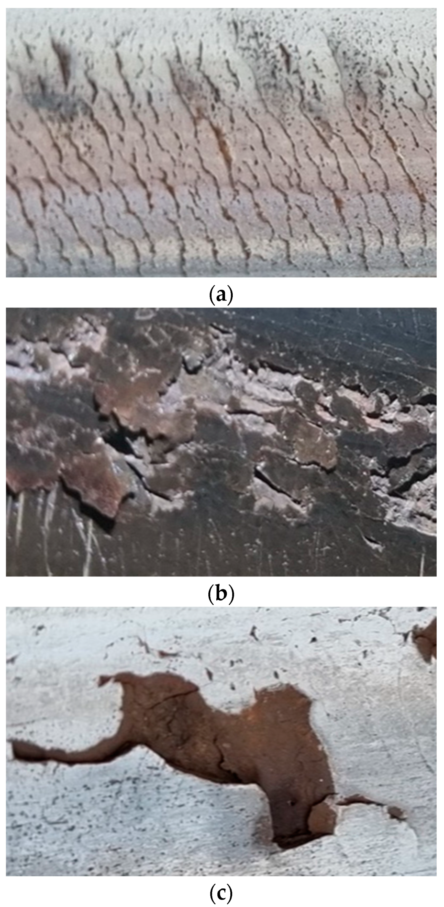
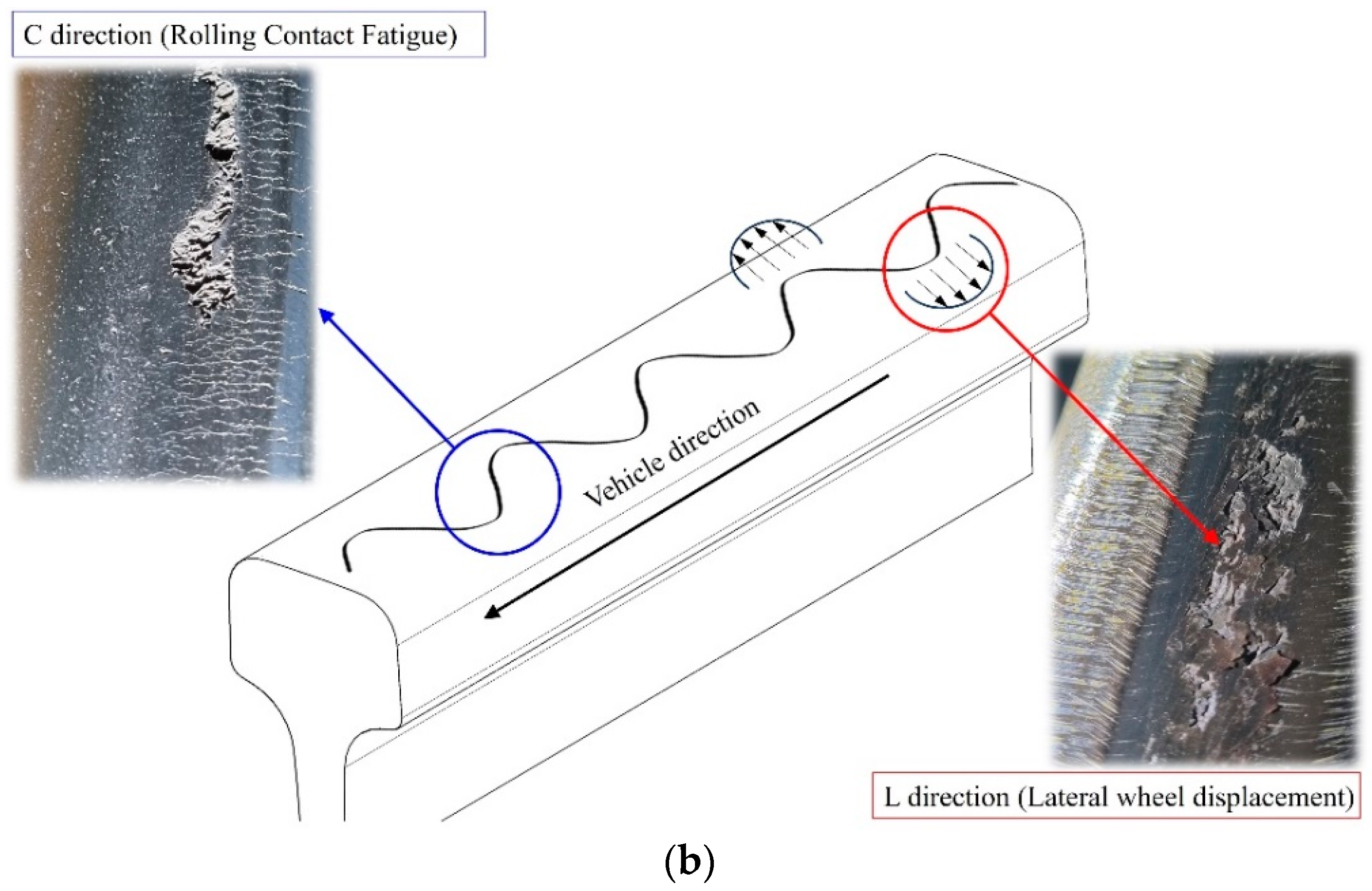
3. Rail Internal Defects Specificity, Characteristic

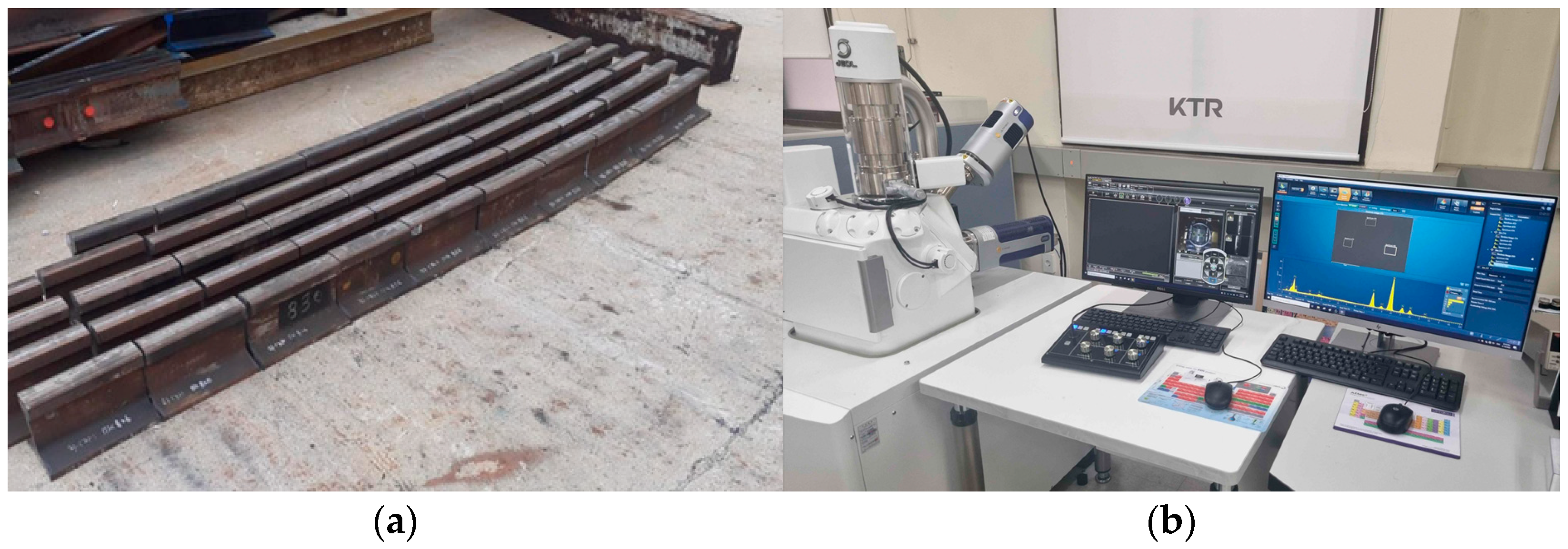
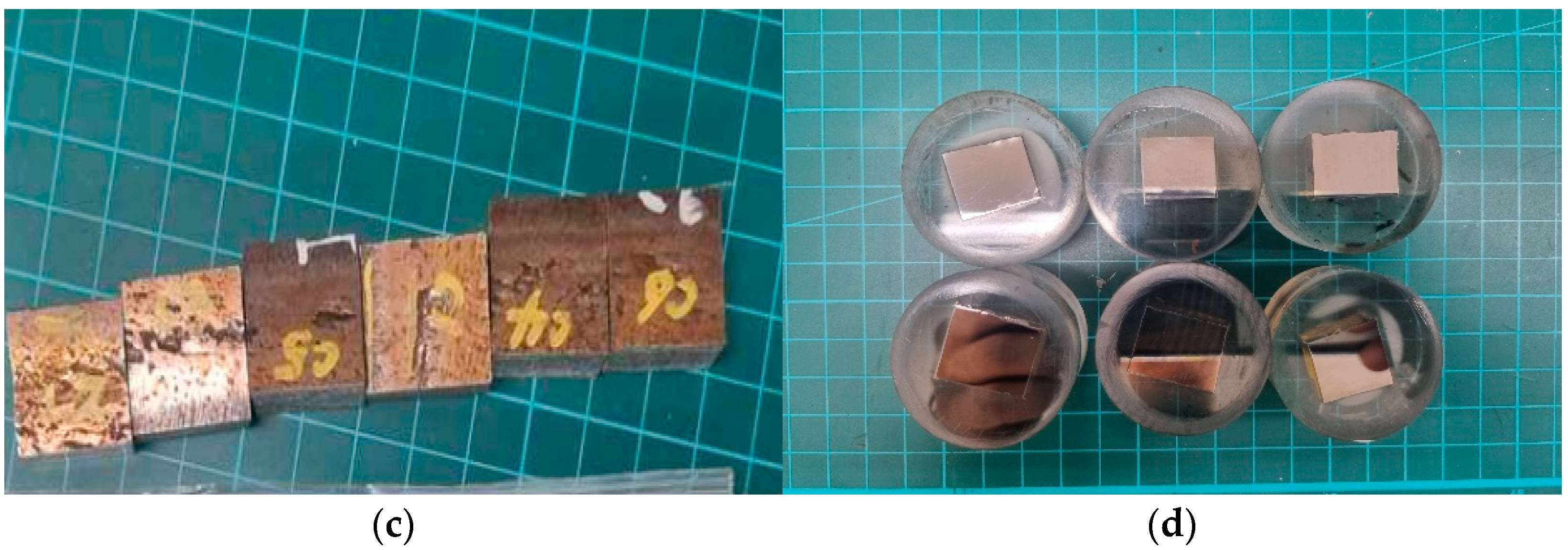
3.1. Overview

Rail surface damage on the currently operational tracks may exhibit various magnitudes and types. Previous studies have mainly focused on investigating the impact of factors, such as the magnitude of wheel–rail contact load and stress variations due to contact area, on the formation of cracks or damages on the rail surface. An inspector faces various difficulties in visually detecting rail surface damage when inspecting from a long distance. Upon conducting an extensive examination of the affected area, it was determined that the rail surface damage may yield different results depending on the perspective of the inspector. This study analyzed rail internal defects occurring at various depths and lengths in such surface damages through SEM testing.

The flowchart of the SEM test procedure is illustrated in Figure 3. The damaged rails were sampled through field investigation. An analysis was conducted to distinguish the types of damage based on the examination of the characteristics of cracks that extend from the rail surface into the interior of the rail. The surface defects on the rail surface, which occur in the direction of the train travel due to wheel–rail contact (rolling contact fatigue, RCF), are classified into two types: rolling direction (C) defects caused by the contact, and lateral wheel displacement direction (L) defects caused by the lateral movement of the wheels. In addition, an SEM test was conducted.

The conical wheel shape of the train’s wheel axle is crucial in terms of the contact with the rail. The turning radius of a vehicle may vary, and the rolling contact occurs in varying degrees when the wheel and rail surfaces are in contact. This study investigated the phenomenon of non-uniform crack patterns resulting from wheel–rail contact in the field. The damage characteristics of patterns with different crack orientations were investigated through SEM testing.

In the field measurement of this study, rail samples (7–15 m) with damaged rail surfaces were collected from an operational urban railway service. A total of 100 specimens were cut at 30 cm intervals. In the SEM testing, damaged rail specimens were processed to demonstrate the correlation between surface defects and internal defects (cracks). Surface defect-specific specimens were processed and mounted, and they were then polished to measure the depth, length, and angle of the cracks. The crack angle indicates the rate of growth of a crack that progresses in a certain direction of length [6,7,8].

In this study, the cross-sectional observation was performed on each sample by cutting it in the appropriate direction and mounting the cross-section. After mounting, polishing was carried out using 1 μm diamond suspension. The crack length, depth, and angle were measured using an electron scanning microscope (JEOL JSM-IT500 with OXFORD ULTIM MAX). Figure 4 shows an examination of rail tissue and equipment test using scanning electron microscopy (SEM).

There are some challenges in the measurement of rail-internal cracks using non-destructive testing. The level of rail surface damage was quantified, and the correlation between surface and internal defects was accordingly examined. The processed sample shown in Figure 4a was observed via SEM using the setup shown in Figure 4b. To demonstrate the correlation between surface defects and internal defects (cracks) in aged rail specimens, damaged rail observations were conducted by processing the rail samples, as shown in Figure 4c,d, The damaged rail is presented in Figure 4c. For cutting, a mechanical cutting method was applied to process the sample to 20 mm × 20 mm or less in the area containing the crack. To grind or polish the cut specimen, as shown in Figure 4d, it was made into a certain shape using a resin; this process is called mounting. The purpose of mounting is to protect the edges and surface of the specimen, fill the pores of porous materials, and make specimens of various shapes into a consistent size that is easy to handle. Mounting methods are largely divided into hot and cold mounting methods and are selectively used depending on the specimen and purpose of use. In this study, the hot mounting method was applied [23]. SEM tests were performed to measure the crack depth, length, and angle.

In addition, the fracture length, crack depth, and crack angle (crack propagation rate) were measured using the SEM test, as shown in Figure 5. Approximately 1300 rail internal defects were measured on the damaged rails. The representative images of damage are depicted in Figure 6.

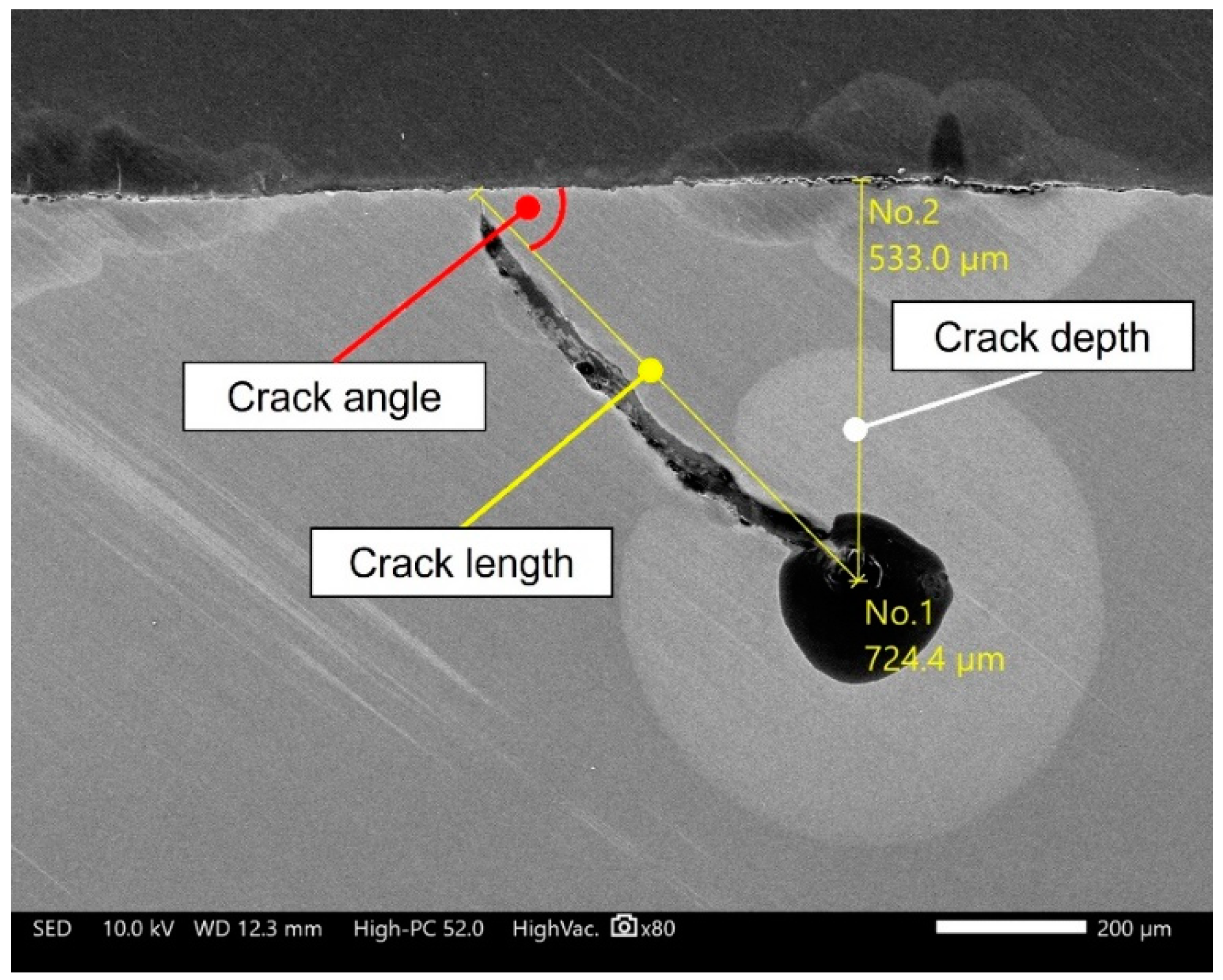
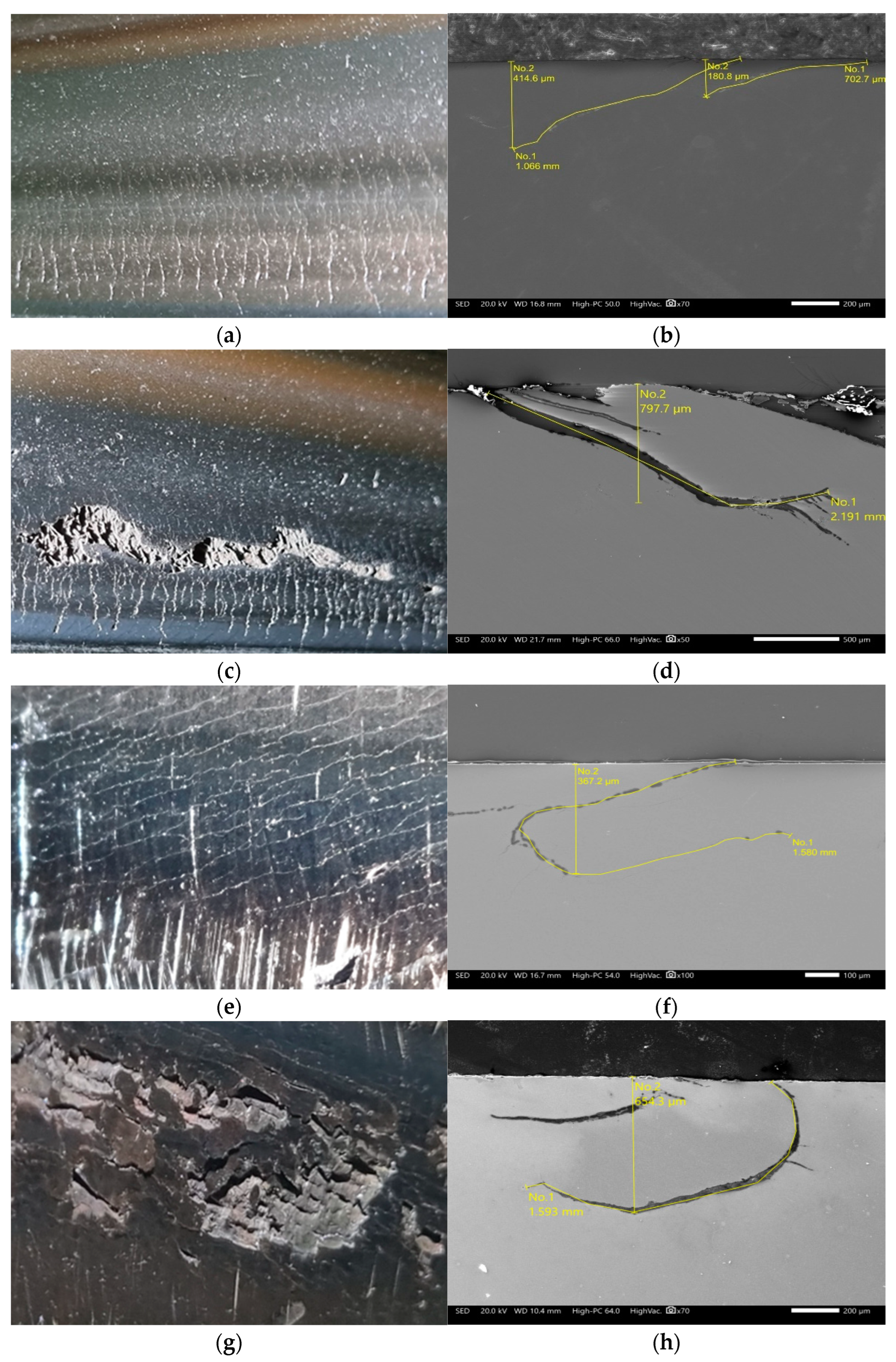
3.2. SEM Test Results

In this study, we used the damaged rail presented in Section 2. For the samples, images of rail surface defects were obtained at various points investigated in the field. Through field investigation, 1300 images of rail surface defects were obtained. Aged rails collected from the field were processed, and 1300 images of internal defects were generated through SEM testing. Therefore, a total of 1300 pieces of learning data were constructed; an example of learning data is illustrated in Figure 6. We classified rail surface defects using a deep learning model based on the constructed learning data.

The defects occurring in the lateral direction of the rail may be attributed to the rolling contact between the wheels and the rail in the direction of train travel, as shown in Figure 6a,b. The SEM test revealed the presence of several defects progressing from the rail surface to its core.

The defects occurring in the longitudinal direction of the rail may be attributed to hunting phenomena and lateral movement of the wheels, as shown in Figure 6c,d. The SEM test results revealed that cracks propagate from the rail surface and grow at an angle that leads them back to the surface.

The scale of rail surface damage (crack depth, length, and angle (crack propagation rate)) was calculated and represented according to the SEM test results. The total number of measured internal defects in the rail was around 1300. These data were plotted as shown in Figure 7.

The correlation between the crack characteristics and rail internal defects was analyzed using the SEM test. The correlation between crack length and crack propagation rate, which was analyzed according to both the C- and L-direction damages, indicated a high level of dispersion in the results, making it difficult to analyze the correlations, as shown in Figure 7. Thus, this study analyzed the correlation of internal damages in rails using the Gaussian probability density technique.

4. Analysis and Discussion

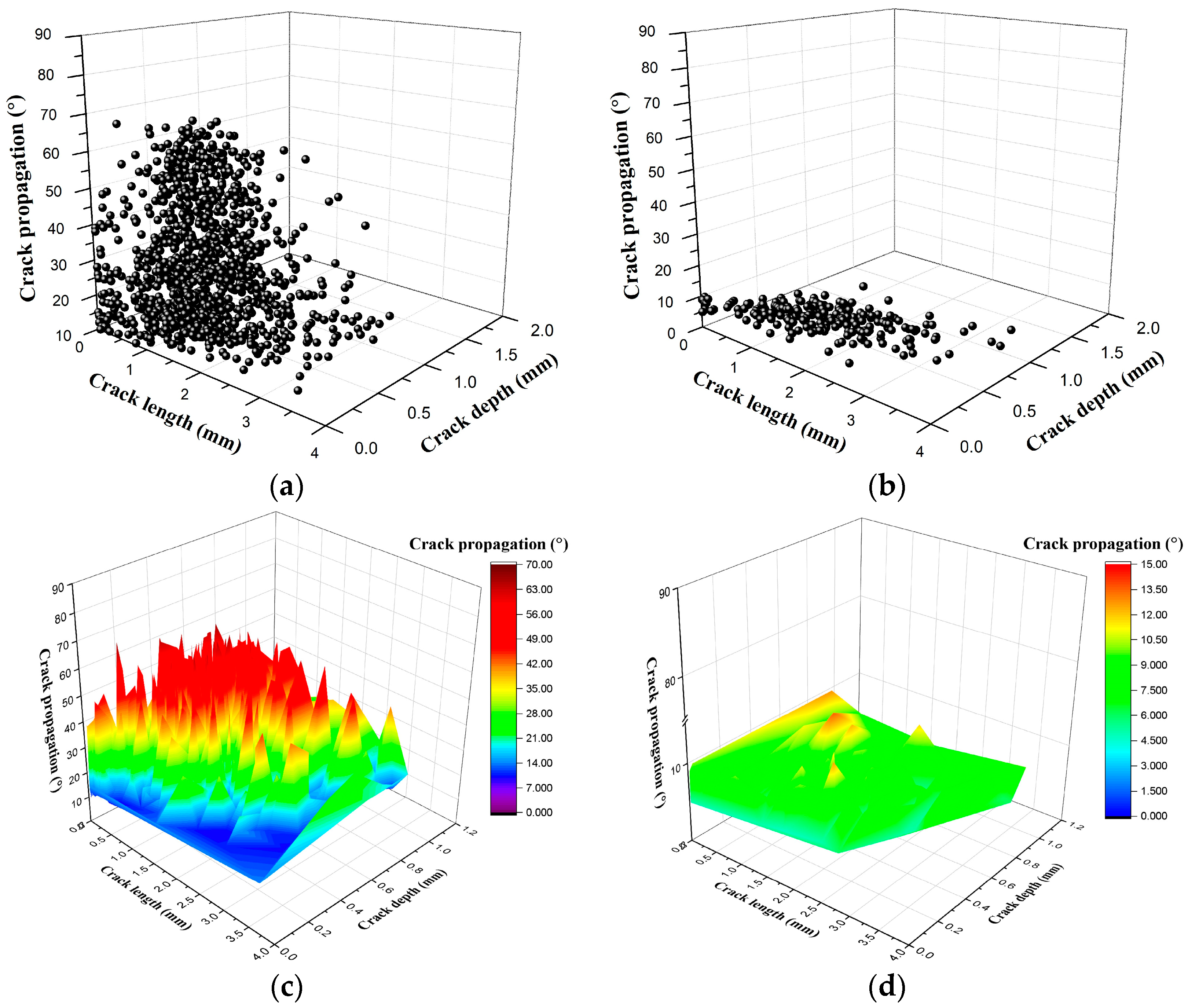
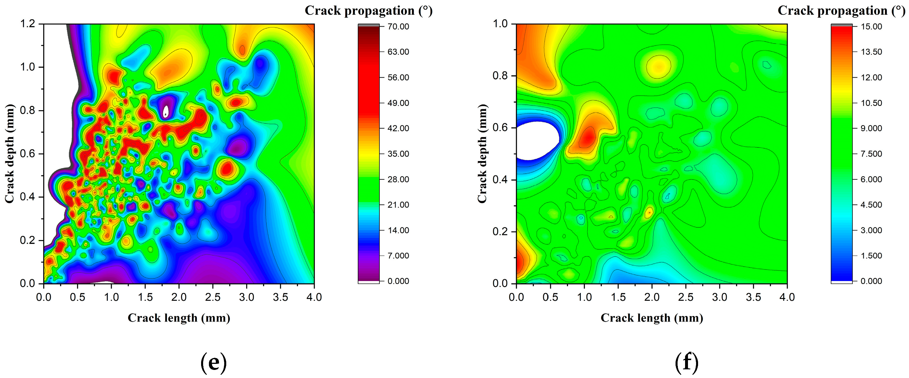
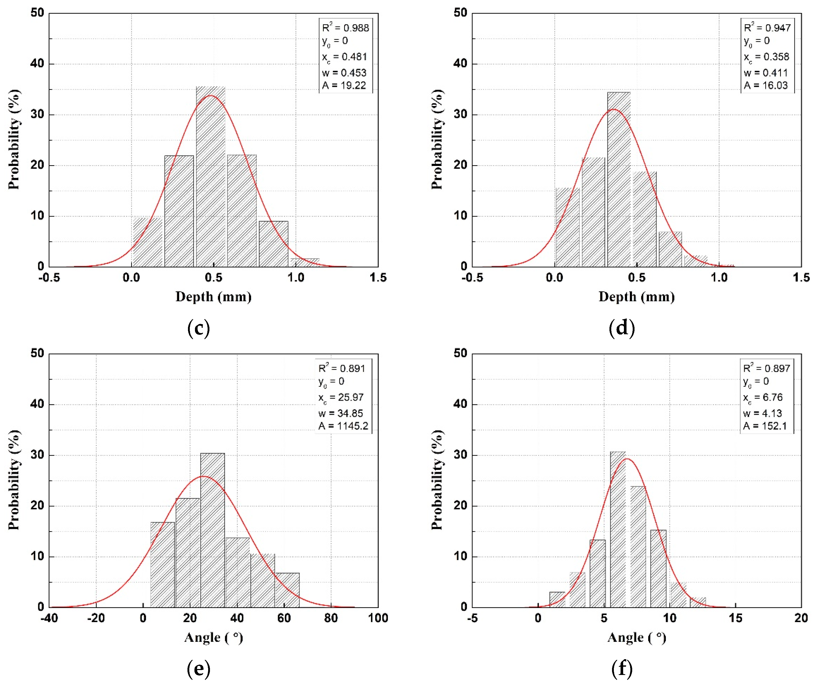
4.1. Gaussian Probability Density Analysis of Rail Internal Defects

The Gaussian distribution is a bell-shaped curve. For a clear understanding of the normal distribution, the definitions of “$x_c$ (mean)”, “$w$ (Standard Deviation)”, and “$A$ (Area)” must be known. Here, “$x_c$” is the calculated average of all values, the “$w$” is the value that represents the range of standard deviation based on the mean, “$A$” refers to the area of the graph and is required to calculate $y_c$, which is the maximum value on the y-axis ($x_c$ = $y_c$) [24].

In this study, the crack angle (crack propagation rate), according to the rail internal damage depth and crack length, was analyzed using the Gaussian probability density function.

The analysis of crack length revealed that in the case of $x_c$, the length in the C direction was 0.902 mm, whereas that in the L direction was 1.504 mm, indicating that the crack length in the L direction was greater than that in the C direction by a factor of 1.67, as shown in Figure 8a,b. Furthermore, in the case of $w$, the C direction exhibited a deviation of ±0.436 mm, whereas the L direction exhibited a deviation of ±0.835 mm. The crack length in the L direction was 1.92 times greater than that in the C direction.

The analysis of crack depth revealed that, in the case of $x_c$, the depths of the crack were 0.481 and 0.358 mm in the C and L directions, respectively, as shown in Figure 8c,d. The crack depth in the C direction was determined to be greater than that in the L direction by a factor of 1.34. Furthermore, in the case of $w$, the length in the C direction exhibited a deviation of ±0.227 mm, whereas that in the L direction exhibited a deviation of ±0.206 mm. It was observed that the crack depth in the C direction was greater than that in the L direction by a factor of 1.10.

The analysis of the crack angle (crack propagation rate) revealed that, in the case of $x_c$, the crack angle in the C direction was 25.97°, while that in the L direction was 6.76° mm. It was determined that the fracture angle in the C direction was larger than in the L direction by a factor of 3.84. Furthermore, in the case of $w$, the crack angle in the C direction exhibited a ±17.43° deviation, while that in the L direction exhibited a ±0.206 mm deviation. The crack angle (crack propagation rate) in the C direction was higher than that in the L direction by a factor of 1.10.

The characteristics of rail internal defects manifested as damages of various lengths within the range of a significant standard deviation. As shown in

Table 1. Analysis results of rail internal crack characteristics.

Division	Crack Depth (mm)	Crack Length (mm)	Crack Propagation Angle (°)
C direction	0.481 (±0.227) 0.254–0.708	0.902 (±0.436) 0.466–1.338	25.97 (±17.43) 8.54–43.4
L direction	0.358 (±0.206) 0.152–0.564	1.504 (±0.835) 0.669–2.339	6.76 (±2.07) 4.69–8.83

, An analysis revealed that the average value ($x_c$) of the damage depth in the C direction was higher than the damage in the L direction. Furthermore, the crack length in the L direction exhibited a relatively large average and standard deviation compared with the crack length in the C direction. It was observed that the large distribution of standard deviation, which is relative to the mean value, indicates the occurrence of significant rail internal defects that have progressed beyond the average level. In terms of the surface damage in the L direction, the defects were observed during curved track conditions. Therefore, it was analyzed that rail surface maintenance should be performed periodically to address the damage in the L direction, which occurs more frequently than the damage on straight tracks. The characteristics of damage length, depth, and crack growth rate were determined according to this probability distribution. Furthermore, depending on the direction of rail surface damage that occurs in urban railways, the size of the defect leading to the interior varies and appropriate maintenance is necessary to manage this.

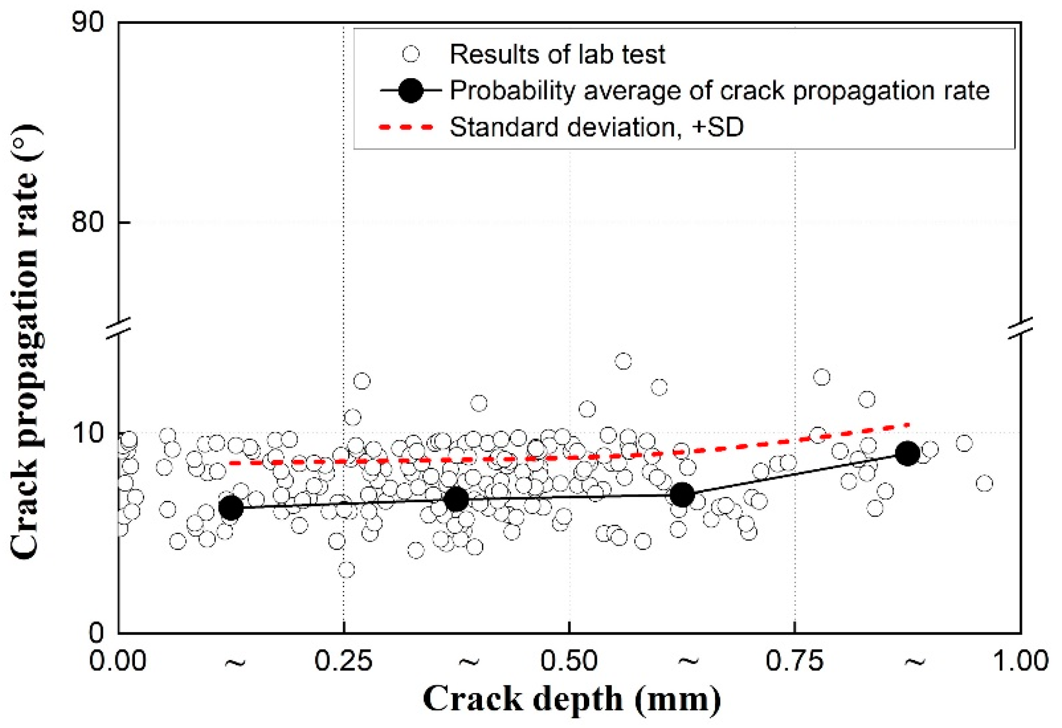
4.2. Gaussian Probability Density Function Analysis According to Crack Depth

This study analyzed the correlation between crack propagation rate and crack depth based on the Gaussian probability density function. The correlation between crack depth and crack propagation rate, according to the direction of damage, is illustrated in Figure 9 and Figure 10, as well as in

Table 2. Crack propagation rate analysis results according to rail crack depth (C direction).

Crack Depth Range	Crack Propagation Probability Average Value (Xc, mm)	Standard Deviation (SD, mm)	Crack Propagation Angle (°)
0.00–0.25 mm	18.2	±9.43	8.77–27.63
0.25–0.50 mm	21.34	±14.10	7.24–35.44
0.50–0.75 mm	30.46	±19.9	10.56–50.36
0.75 mm<	25.12	±12.27	12.85–37.39

and

Table 3. Crack propagation rate analysis results according to rail crack depth (L direction).

Crack Depth Range	Crack Propagation Probability Average Value (Xc, mm)	Standard Deviation (SD, mm)	Crack Propagation Angle (°)
0.00–0.25 mm	6.28	±2.23	4.05–8.51
0.25–0.50 mm	6.71	±1.98	4.73–8.69
0.50–0.75 mm	6.93	±1.89	5.04–8.82
0.75 mm<	9.01	±1.42	7.59–10.43

.

The analysis of crack angle (crack propagation rate) according to the depth of rail sur-face cracks revealed that the crack propagation rate and standard deviation increased and then gradually decreased as the crack depth increased, as shown in Figure 9. It was further observed that the fracture propagation rate exhibited the highest standard deviation for crack depths, ranging from 0.50 mm to 0.75 mm. Furthermore, it was inferred that, at crack depths larger than 0.75 mm, there was a slight attenuation in both the standard deviation and range of the crack propagation rate. Therefore, the range 0.50–0.75 mm was found to be the critical level in terms of fracture propagation rate.

As shown in Table 2, it was observed that the relative difference of $x_c$ in the range 0.25–0.50 mm increased by approximately 17% compared with that in the range 0–0.25 mm, and the relative difference of the standard deviation increased by approximately 49.5%. The relative difference of $x_c$ increased by approximately 42.74% in the range 0.50–0.75 mm compared with 0.25–0.50 mm, and the relative difference of the standard deviation increased by approximately 41.1%. The relative difference of $x_c$ decreased by approximately 17.53% in the range of 0.75 mm and above, whereas the relative difference of the standard deviation decreased by approximately 38.4%.

The analysis of crack angle (crack propagation rate) according to the depth of rail sur-face cracks revealed that the average and range of crack propagation rate increase with the fracture depth. The range of fracture propagation rate was the highest in cases where the crack depth was equal to or greater than 0.75 mm. In contrast, it was observed that the standard deviation range of crack propagation rate for intervals 0–0.75 mm or higher decreased.

As shown in Table 3, the relative difference of $x_c$ in the range 0.25–0.50 mm increased by approximately 6.85% compared with that in 0–0.25 mm. Additionally, the relative difference of the standard deviation decreased by approximately 11.2%. The relative difference of $x_c$ increased by approximately 3.28% in the range 0.50–0.75 mm compared with that in 0.25–0.50 mm, whereas the relative difference of the standard deviation decreased by approximately 4.5%. The relative difference of $x_c$ increased by 30% in the range of 0.75 mm and above, whereas the relative difference of the standard deviation decreased by approximately 24.9%. The RCF damage observed in this study can be broadly classified into two types: C-direction damage and L-direction damage. Additionally, differences in defect characteristics depending on the damage direction can be identified using Gaussian probability density analysis. Therefore, as a result of the rail surface defect analysis using the Gaussian probability density function performed in this study, C-direction damage characteristics with a relatively high crack growth rate were analyzed. Through indoor testing, we determined that damage to the rail surface must be removed before reaching an internal crack depth of approximately 0.5 mm or more. The rail internal damage characteristics showed damage of various lengths within the standard deviation size. In the case of surface damage in the L direction, it mainly occurs during curved driving conditions; therefore, we determined that rail surface management should periodically manage the rail surface where damage in the L direction occurs rather than on a straight road. Through this probability distribution, the characteristics of damage length, depth, and crack growth rate were identified. In addition, we believe that it can be used for rail surface maintenance and management by setting it as a threshold value for cracks that occur in urban railways.

5. Rail Surface Damage Deep Learning Model

5.1. Introduction

This study obtained around 1300 training datasets by matching rail surface photos and rail internal damage images in the rail surface damage section of an operational urban railway. The algorithm used in this study not only used training data, but also proceeded with the commonly used ratio of learning (80%), verification (10%), and testing (10%). The investigation of the condition of rail internal cracks originating from the rail surface using non-destructive testing methods was challenging. This study developed a deep learning model that utilizes training data to quantitatively represent the condition of rail internal defects using just rail surface images and to derive defects that are difficult for inspectors to investigate.

The training data were classified based on the two main types of rail surface damage, headcheck and spalling, which are representative forms of RCF damage, as shown in Figure 7. Furthermore, rail surface damage images with crack depths in the range 0–0.5 mm for rail internal defects were classified and identified as Headcheck_A. Furthermore, Head-check_B was quantified and classified based on crack depths of 0.5–0.75 mm or larger.

The rail surface damage images with crack depths of 0–0.5 mm were classified and identified as Spalling_A. In addition, Spalling_B, with a crack depth of 0.5–0.75 mm or more, was quantified and classified as a training dataset.

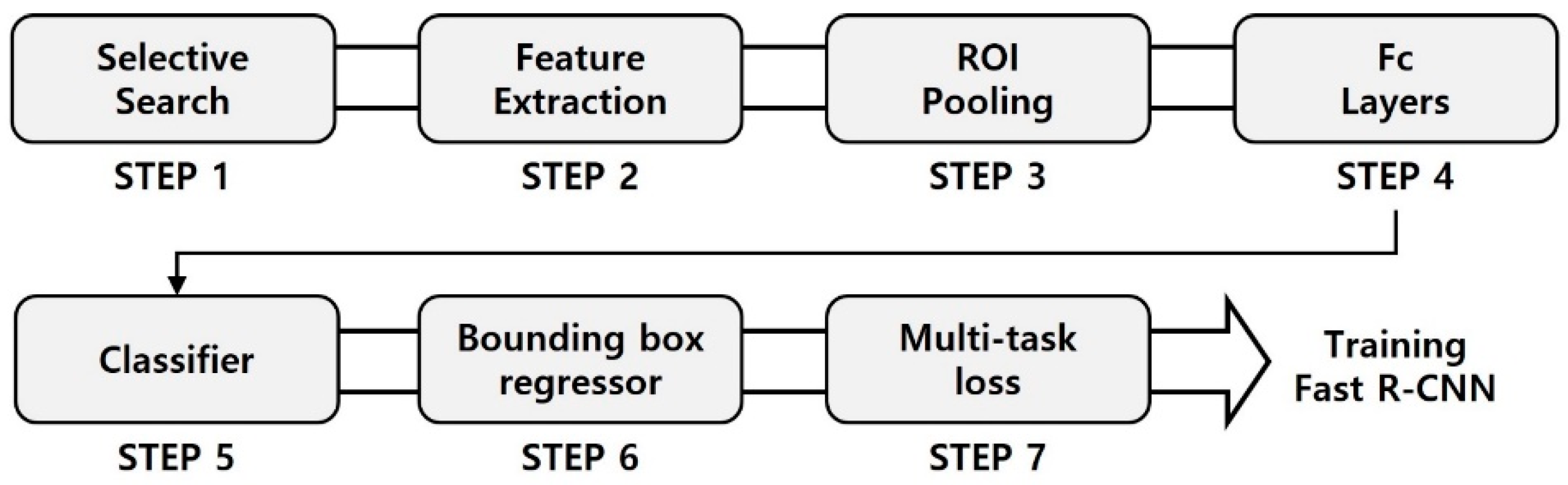
5.2. Fast R-CNN (Regional Convolutional Neural Network)

When photos with cracks are input to the Fast R-CNN, as shown in Figure 11, the features are extracted using CNN and then passed to the region proposal network (RPN) and the object classifier for object recognition [25,26,27,28,29,30,31,32,33,34]. The RPN generates multiple candidate regions and objectivity scores to propose the locations of objects within the input image. An object detector utilizes the region of interest (ROI) pooling to adjust object candidate regions of different sizes proposed by RPN to a uniform size, and it then classifies based on the object they belong to. The detected objects are output as bounding boxes.

The use of an analysis technique that applies deep learning to rail surface damage image data may help minimize human errors, unlike traditional visual inspection. This will provide administrators and inspectors with reliable and significant data for diagnosing rail surface damage and enable highly accurate analysis.

5.3. Fast R-CNN Model Training and Prediction

The training method of the Fast R-CNN model used in this study is illustrated in Figure 12, and the model training and prediction were performed in a step-by-step manner [25,26].

The method of training a model in Fast R-CNN when a single image is input to the training dataset is as follows. The selective search algorithm is used to extract region proposals, as shown in Step 1 in Figure 12. Two thousand region proposals were extracted from one image. For feature extraction in Step 2, 512 feature maps of size 14 × 14 are extracted using the VGG16 model to input images of size 224 × 224 × 3. In Step 3, the ROI pooling is performed on the extracted feature map by conducting ROI projection and applying the Max pooling method, which results in the extraction of 512 feature maps of size 7 × 7.

In Step 4, the fully connected (fc) layers flatten the extracted 7 × 7 × 512 feature map and generate a feature vector of size 4096 through the fc layer. In Step 5, the classifier inputs the generated feature vector of size 4096 into an fc layer with five output units, including four classes, as well as the background. Furthermore, the process involves obtaining class predictions for a single region proposal in a given image.

In Step 6, the bounding box regressor considers a feature vector of size 4096 and predicts the coordinates of the bounding box for each class. This is achieved by inputting the feature vector into a fully connected layer with 5 × 4 output units. Furthermore, bounding box coordinates for each class are obtained from one image. In Step 7, the multi-task loss returns the loss of the classifier and bounding box regressor for a single area proposal. Then, both the classifier and bounding box regressor models are trained simultaneously through backpropagation.

5.4. Experiment Environment

The experiment was based on Python version 3.9.16 in the integrated development environment (IDE) PyCharm 2021.3. Additionally, the experiment was conducted using a computer featuring Windows 10 OS, i7-10700 CPU, NVIDIA GeForce RTX 3070 GPU, and 64 GB RAM, as shown in

Table 4. Experiment environment.

Division	Environment
OS	Windows 11 Professional
CPU	Intel(R) Core (TM) i5-13600K CPU @ 3.5GHz
RAM	DDR5 32G(PC5-44800) * 4 = 128G
GPU	GeForce RTX 4060Ti
SSD	Gold P31 M.2 2TB

. The Fast R-CNN model was used to classify damaged surfaces. The model utilized Keras (v2.9.0), an open source neural network library written in Python. CUDA v12.2 was used for GPU use during training, and cuDNN v8.9.0, a GPU-specific library, was used.

The true positive (TP), true negative (TN), false positive (FP), and false negative (FN) were calculated from the results of classifying the validation data, and the three performance metrics were applied accordingly. Here, TP refers to the cases where the model correctly identifies a crack image as positive, FP refers to the case where the model incorrectly identifies a crack image as positive. Furthermore, FN refers to the case where the model incorrectly identifies a non-crack image as positive, while TN refers to the case where the model correctly identifies a non-crack image as negative. The methods for calculating performance indicators are summarized in

Table 5. Confusion matrix.

		Correct Answer
		True	False
Classification result	True	True Positive	False Positive
	False	False Negative	True Negative

.

The performance of the object detection algorithm was evaluated using a confusion matrix. In Table 5, TP represents correct detection, FP represents the case where an item that must be detected was not detected, FP represents incorrect detection, and TN represents the case where an item that must not be detected was detected. The concepts of Recall, Precision, and Accuracy were summarized in terms of TP, FP, FN, and TN.

Recall is the ratio of items correctly detected to be true by the model to the actual true values. Recall can also be defined as the ratio of rail surface damage that the model predicted as cracks among the actual correct answers. It can be expressed as follows:

$$Recall= \frac{TP}{TP+FN}$$

(1)

Precision is the ratio of items detected to be true by the model that are actually true, and it can be expressed as follows:

$$Precision= \frac{TP}{TP+FP}$$

(2)

Accuracy evaluates the ratio of correct predictions out of the total predictions made. The values were examined and analyzed to increase the Accuracy. Accuracy can be ex-pressed as follows:

$$Accuracy= \frac{TP}{TP+FN+TN+FP}$$

(3)

Performance evaluation assesses the suitability of a deep learning model using Recall, Precision, and Accuracy.

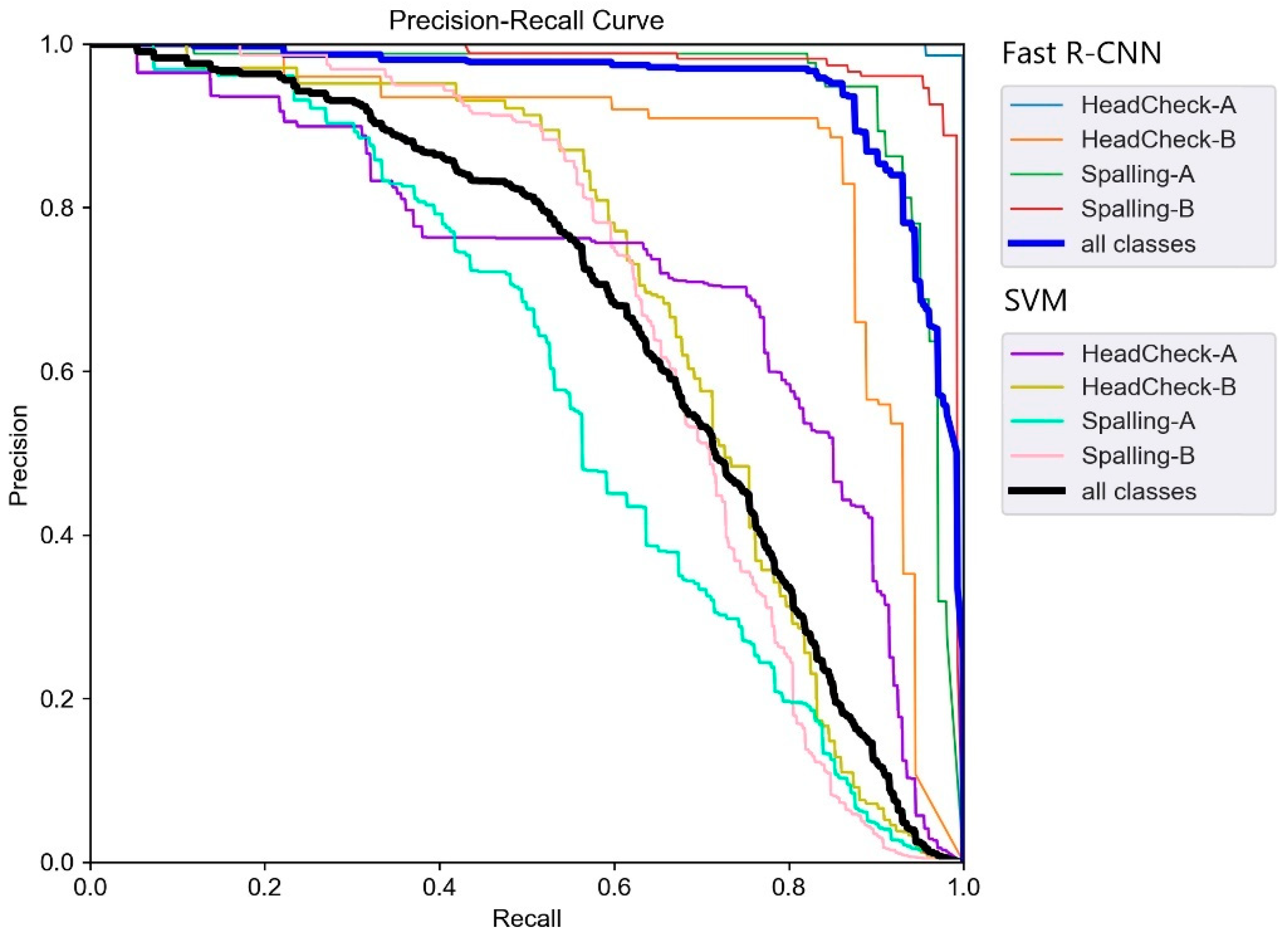
5.5. Experimental Result

This study obtained the Precision–Recall curve by calculation, as shown in Figure 13. The ordinate and abscissa represent the Precision and Recall, respectively. Furthermore, in the case of multiple object classes, the performance of the algorithm is evaluated by calculating the average precision (AP) for each class and then summing them all up, which is then divided by the number of object classes. This is referred to as the mean average precision (mAP). The suitability of the deep learning model is evaluated as shown in Figure 13. The model’s precision is high, but if the recall is low, although the model may accurately classify objects as correct, it may only classify a subset of the correct predictions. Therefore, while it is accurate to classify it as rail surface damage, there is a high likelihood that it is not a crack but something else. The model exhibits high recall but low precision, meaning that it correctly classifies a majority of the true positives but also misclassifies many false positives. The configured dataset was analyzed for the ratio of mAP.

In this study, test results between SVM and Fast R-CNN were compared, as shown in

Table 6. Comparison of test results between SVM and Fast R-CNN.

Learning Data	Model (mAP ([email protected]))
	Fast R-CNN	SVM
Headchek_A	99.4	72.0
Headchek_B	86.8	70.1
Spalling_A	95.3	58.4
Spalling_B	98.2	68.2
All classes	94.9	67.2

. The analysis results using the SVM model demonstrated that Headcheck_A and Headcheck_B exhibited analysis scores of 72% and 70.1%, respectively.

Spalling_A and Spalling_B were analyzed and were observed to exhibit values of 58.4% and 68.2%, respectively. The deep learning model used in this study was employed to analyze the rail surface damage images for the entire class. The mean average precision (mAP) value was 67.2%. Therefore, the suitability of this model as a detector for rail surface cracks has been analyzed to be low.

The analysis results using the Fast R-CNN model exhibited high accuracy for Head-check_A and Headcheck_B, yielding values of 99.4% and 86.8%, respectively. However, in the case of Headcheck_B, the accuracy is 86.8%. During the implementation phase, acquiring additional training data is deemed necessary to achieve higher accuracy.

Spalling_A and Spalling_B were observed to yield detection accuracies of 95.3% and 98.2%, respectively, indicating a high level of accuracy in detecting cracks. Furthermore, the image analysis of rail surface damage for the entire class using the deep learning model in this study revealed an mAP value of 94.9%. This indicates that the model’s suitability has been ensured.

A comparative analysis of SVM and Fast R-CNN reveals that the relative difference is approximately 41%, indicating that the Fast R-CNN model exhibits higher accuracy in terms of detecting rail surface defects compared to the SVM model. An analysis revealed that the Fast R-CNN model was more beneficial in terms of identifying rail surface defects.

This study aimed to develop an application for rail surface damage that can be used in actual diagnostic tasks. To this end, the criteria for rail surface damage from the Detailed Guideline on the Performance Evaluation of Track Facilities were used to classify and integrate the training dataset. Furthermore, machine learning algorithms were used to train the evaluation criteria and convergence point for rail surface damage.

6. Conclusions

This study involved collecting rail samples through on-site investigation in sections where rail surface defects occurred. Furthermore, an analysis was conducted to examine the characteristics of rail internal defects based on an indoor SEM Test. The training data were constructed based on images of rail surface defects obtained through on-site investigation and data of rail internal defects obtained through SEM testing. Furthermore, a deep learning algorithm was developed by distinguishing the classes based on headcheck and spalling. We developed a deep learning model for diagnosing rail surface damage using the Fast R-CNN algorithm.

In this study, we developed a deep learning model that can diagnose rail internal defects using rail surface damage. In the field investigation, rail surface damage was investigated, and in the indoor test, SEM testing was used to construct image data of rail internal damage. Crack length, depth, and angle were quantified based on the indoor test results.

The deep learning model used in this study indicated that the Fast R-CNN yielded a higher accuracy compared with the SVM model. The rail surface defects were detected through the creation of a dataset, configuration of model parameters, and training of the model. The analysis of the test results led to the conclusion that rail surface defects can be detected and the types of defects may be effectively identified. Furthermore, it was concluded that this will greatly contribute to reducing railway accidents.

The deep learning model used in this study can replace the subjective evaluations based on human resources and provide the management with predictive and diagnostic data according to big data. It has been determined that ensuring the safety of the citizens; enhancing technology through safety specialization; and addressing the costly maintenance, reinforcement, and collisions caused by accidents may be resolved through a proactive diagnostic system. The aim was to enhance cost savings and improve the value of data utilization, rather than relying on traditional maintenance and inspection methods (such as labor costs and visual inspections). The use of an analysis technique wherein deep learning is applied to rail surface damage image data is expected to minimize human errors, unlike traditional visual inspection. This will provide administrators and inspectors with reliable and significant data for diagnosing rail surface damage and enable highly accurate analyses.

The social damages resulting from major accidents can be minimized by identifying the possibility of fractures based on rail surface damage. The findings of this study suggest that it will be possible to scientifically trace the history of track damage and increase the reliability of track diagnosis results by converting the rail damage condition and inspection history into big data.

In future research, we plan to develop a diagnostic application that can diagnose rail internal defects using rail surface damage. In this study, we aimed to apply a deep learning model (Fast R-CNN) using image data constructed from field surveys and indoor tests to applications. By developing a rail surface damage diagnosis application (app) using a deep learning model that can be used on smart devices, we plan to perform smart diagnoses of rail surface damage that can be used in track diagnosis and performance evaluation work in South Korea in the future.

In the current research stage, a deep learning model that classifies rail surface conditions and predicts rail internal defects was studied using the Fast R-CNN model. In future research, we plan to change the deep learning model or subdivide the training data set and derive a comparison method between models by reflecting not only performance but also calculation time.

References

1. Choi, J.Y. Qualitative Analysis for Dynamic Behavior of Railway Ballasted Track. Ph.D. Thesis, Technical University of Berlin, Berlin, Germany, 2014. [Google Scholar]
2. Choi, J.Y.; Park, D.R.; Chung, J.S.; Kim, S.H. Dynamic wheel-rail force-based track-irregularity evaluation for ballasted track on serviced railway by adjacent excavation. Appl. Sci. 2022, 12, 375. [Google Scholar] [CrossRef]
3. Gren, D.; Ahlstrom, J. Fatigue Crack Propagation on Uniaxial Loading of Biaxially Predeformed Pearlitic Rail Steel. Metals 2023, 13, 1726. [Google Scholar] [CrossRef]
4. Constantin-Ioan, B.; Corneliu, M.; George-Radu, P.; Lorenz, P.; Daniela-Lucia, C.; Cătălina, A.; Andreea-Carmen, B. Determining the causes that led to a railway rail breaking. In Railway infrastructure development for an efficient & green transport; Railway PRO: Edinburgh, UK, 2011; pp. 5–9. [Google Scholar]
5. Grassie, S.L. Rail Corrugation: Characteristics, Cause and Treatments. Proc. Inst. Mech. Eng. Pt. F J. Rail Rapid Transit 2009, 223, 581–596. [Google Scholar] [CrossRef]
6. Damme, S.; Nackenhorst, U.; Wetzel, A.; Zastrau, B.W. On the Numerical Analysis of the Wheel-Rail System in Rolling Contact. In System Dynamics and Long-Term Behaviour of Railway Vehicles, Track and Subgrade; Springer: Berlin/Heidelberg, Germany, 2003; Volume 6, pp. 155–174. [Google Scholar]
7. Baeza, L.; Thompson, D.J.; Squicciarini, G.; Denia, F.D. Method for Obtaining the Wheel–Rail Contact Location and Its Application to the Normal Problem Calculation through ‘CONTACT’. Veh. Syst. Dyn. 2018, 56, 1734–1746. [Google Scholar] [CrossRef]
8. Franklin, F.J.; Weeda, G.-J.; Kapoor, A.; Hiensch, E.J.M. Rolling Contact Fatigue and Wear Behaviour of the Infrastar Two-Material Rail. Wear 2005, 258, 1048–1054. [Google Scholar] [CrossRef]
9. Conner, B.P. Contact Fatigue: Life Prediction and Palliatives. Ph.D. Thesis, Massachusetts Institute of Technology, Cambridge, MA, USA, 2016. [Google Scholar]
10. Donzella, G.; Mazzù, A.; Petrogalli, C. Competition between Wear and Rolling Contact Fatigue at the Wheel—Rail Interface: Some Experimental Evidence on Rail Steel. Proc. Inst. Mech. Eng. Pt. F J. Rail Rapid Transit 2009, 223, 31–44. [Google Scholar] [CrossRef]
11. Steyn, E. Rail Surface Treatment Grinding and Milling—Competing or Complementary Technologies. Master’s Thesis, Chalmers University of Technology, Gothenburg, Sweden, 2019. [Google Scholar]
12. Mihai, D.M. Efficient Solutions for Diminuting the Rolling Noise of Trains. In Railway infrastructure development for an efficient & green transport; Railway PRO: Edinburgh, UK, 2011; pp. 50–52. [Google Scholar]
13. Popović, Z.; Lazarević, L.; Mićić, M.; Brajović, L. Critical analysis of RCF rail defects classification. Transp. Res. Procedia 2022, 63, 2550–2561. [Google Scholar] [CrossRef]
14. Zerbst, U.; Lundén, R.; Edel, K.-O.; Smith, R.A. Introduction to the Damage Tolerance Behaviour of Railway Rails—A Review. Eng. Fract. Mech. 2009, 76, 2563–2601. [Google Scholar] [CrossRef]
15. Ndao, B. Generation et Detection sans Contact des ondes de Rayleigh par Methodes Ultrasons-Laser et EMAT Mode Statique et Dynamic Application to the Detection of Surface Defects in the Rail Head. Ph.D. Thesis, University of Valenciennes and Hainaut-Cambresis, Valenciennes, France, 2016. [Google Scholar]
16. Nielsen, J.C.O.; Johansson, A. Out-of-round railway wheels-a literature survey. Proc. Inst. Mech. Eng. Pt. F J. Rail Rapid Transit 2000, 214, 79–91. [Google Scholar] [CrossRef]
17. Ishida, M.; Ban, T.; Iida, K.; Ishida, H.; Aoki, F. Effect of moderating friction of wheel/rail interface on vehicle/track dynamic behaviour. Wear 2008, 265, 1497–1503. [Google Scholar] [CrossRef]
18. Kaewunruen, S. Monitoring structural deterioration of railway turnout systems via dynamic wheel/rail interaction. Case Stud. Nondestruct. Test. Eval. 2014, 1, 19–24. [Google Scholar] [CrossRef]
19. Sresakoolchai, J.; Kaewunruen, S. Detection and severity evaluation of combined rail defects using deep learning. Vibration 2021, 4, 341–356. [Google Scholar] [CrossRef]
20. Yang, Z.; Li, Z. Rail Infrastructure Resilience—Part 7 Wheel-Rail Dynamic Interaction; Elsevier: Amsterdam, The Netherlands, 2022; pp. 111–135. [Google Scholar] [CrossRef]
21. Ministry of Land, Infrastructure and Transport. Guidelines for regular inspection of railway facilities, etc.; Ministry of Land, Infrastructure and Transport: Sejong-si, Republic of Korea.
22. Korea National Railway. Detailed Guidelines on Performance Evaluation of Track Facilities; Korea National Railway: Daejeon, Republic of Korea, 2021. [Google Scholar]
23. Babu, S.R.; Jaskari, M.; Järvenpää, A.; Porter, D. The Effect of Hot-Mounting on the Microstructure of an as-Quenched Auto-Tempered Low-Carbon Martensitic Steel. Metals 2019, 9, 550. [Google Scholar] [CrossRef]
24. Dasgupta, A.; Wahed, A. Clinical Chemistry, Immunology and Laboratory Quality Control; Elsevier: Amsterdam, The Netherlands, 2014; pp. 47–66. [Google Scholar]
25. Perez, L.; Wang, J. The Effectiveness of Data Augmentation in Image Classification using Deep Learning. arXiv 2017, arXiv:1712.04621. [Google Scholar]
26. Ross, G. Fast R-CNN. IEEE International Conference on Computer Vision (ICCV). arXiv 2015, arXiv:1504.08083. [Google Scholar]
27. Jog, G.M.; Koch, C.; Golparvar-Fard, M.; Brilakis, I. Pothole properties measurement through visual 2D recognition and 3D reconstruction. In Proceedings of the International Conference on Computing in Civil Engineering, Clearwater Beach, FL, USA, 17–20 June 2012; pp. 553–560. [Google Scholar] [CrossRef]
28. Buza, E.; Omanovic, S.; Huseinovic, A. A Pothole Detection with Image Processing and Spectral Clustering. In Proceedings of the 2nd International Conference on Information Technology and Computer Networks, Konya, Turkey, 8–10 October 2013; pp. 48–53. [Google Scholar]
29. Mednis, A.; Strazdins, G.; Zviedris, R.; Kanonirs, G.; Selavo, L. Real Time Pothole Detection using Android Smartphones with Accelerometers. In Proceedings of the IEEE International Conference on Distributed Computing in Sensor Systems and Workshops, Barcelona, Spain, 27–29 June 2011. [Google Scholar] [CrossRef]
30. Yin, T.; Yang, J. Detection of Steel Surface Defect Based on Faster R-CNN and FPN. In Proceedings of the International Conference on Computing and Artificial Intelligence (ICCAI), Tianjin, China, 23–26 April 2021; pp. 15–20. [Google Scholar] [CrossRef]
31. Wang, H.; Li, M.; Wan, Z. Rail Surface Defect Detection Based on Improved Mask R-CNN. Comput. Electr. Eng. 2022, 102, 108269. [Google Scholar] [CrossRef]
32. Munawar, H.S.; Hammad, A.W.; Haddad, A.; Soares, C.A.P.; Waller, S.T. Image-based crack detection methods: A review. Infrastructures 2021, 6, 115. [Google Scholar] [CrossRef]
33. Guo, Z.; Wang, C.; Yang, G.; Huang, Z.; Li, G. MSFT-YOLO: Improved YOLOv5 Based on Transformer for Detecting Defects of Steel Surface. Sensors 2022, 22, 3467. [Google Scholar] [CrossRef] [PubMed]
34. Yu, R.; Wei, X.; Liu, Y.; Yang, F.; Shen, W.; Gu, Z. Research on Automatic Recognition of Dairy Cow Daily Behaviors Based on Deep Learning. Animals 2024, 14, 458. [Google Scholar] [CrossRef] [PubMed]
Figure 1. Photograph of the rail damage site.
Applsci 14 01874 g001
Figure 2. Rail surface damages observed during field investigation of urban railway: (a) headcheck; (b) spalling; (c) shell.
Applsci 14 01874 g002
Figure 3. Overview of the SEM test: (a) flowchart of the SEM test; (b) rail surface damage mechanism according to wheel–rail contact conditions.
Applsci 14 01874 g003aApplsci 14 01874 g003b
Figure 4. SEM Test: (a) Rail samples; (b) photograph of the electron scanning microscope; (c) rail sample processing; (d) mounting + polishing.
Applsci 14 01874 g004aApplsci 14 01874 g004b
Figure 5. SEM-test measurement example.
Applsci 14 01874 g005
Figure 6. Deep learning training-data sample (rail surface defects and rail internal defects): (a) rail surface minor defect (C direction); (b) SEM image (Cross cut); (c) rail surface with extended defects (C direction); (d) SEM image (Cross cut); (e) rail surface minor defect (L direction); (f) SEM image (longitudinal cut); (g) rail surface with extended defects (L direction); (h) SEM image (longitudinal cut).
Applsci 14 01874 g006
Figure 7. SEM test results: (a) C direction (All); (b) L direction (All); (c) C direction(3D); (d) L direction (3D); (e) C direction(2D); (f) L direction (2D).
Applsci 14 01874 g007aApplsci 14 01874 g007b
Figure 8. Example of measurement data Gaussian analysis: (a) C direction (length); (b) L direction (length); (c) C direction (depth); (d) L direction (depth); (e) L direction (angle); (f) L direction (angle).
Applsci 14 01874 g008aApplsci 14 01874 g008b
Figure 9. Correlation analysis result between rail surface crack depth and crack propagation rate (C direction).
Applsci 14 01874 g009
Figure 10. Correlation analysis result between rail surface crack depth and crack propagation rate (L direction).
Applsci 14 01874 g010
Figure 11. Fast R-CNN architecture.
Applsci 14 01874 g011
Figure 12. Fast R-CNN training schematic.
Applsci 14 01874 g012
Figure 13. Precision and recall result.
Applsci 14 01874 g013