Article

Impact of the New International Land–Sea Transport Corridor on Port Competition between Neighboring Countries Based on a Spatial Duopoly Model

1
College of Transportation Engineering, Dalian Maritime University, Dalian 116026, China
2
School of Transportation and Logistics, Dalian University of Technology, Dalian 116024, China
*
Author to whom correspondence should be addressed.
Appl. Sci. 2024, 14(5), 1857; https://doi.org/10.3390/app14051857
Submission received: 2 February 2024 / Revised: 17 February 2024 / Accepted: 20 February 2024 / Published: 23 February 2024

Abstract

:
The development of international land–sea transport corridors has provided more convenient access to the sea for inland areas and promoted the improvement of transportation efficiency, environmental improvement, and the strengthening of international cooperation. However, the construction of international land–sea transport corridors has also intensified competition among the ports, which has extended from the local and regional to the national and even international levels. This paper explores the impact of international land–sea transport corridors on oligopolistic port competition between neighboring countries using the Hotelling model. By setting up the utility of the shipper’s port selection, the equilibrium price, market share, and profit of duopoly ports in neighboring countries are analyzed under different conditions of cross-border land transportation and maritime transportation. It is found that the high cross-border transportation cost of the international land–sea transport corridor is not conducive to increasing the market share of the overseas oligopolistic ports in the region. If the maritime transportation cost of overseas oligopoly ports is too high compared with domestic oligopoly ports, it will offset the land transport advantages brought by international land–sea transport corridors. The findings in this paper could provide support for strategic decision making in port markets and cross-border transport corridor development.

1. Introduction

The construction of international land–sea transport corridors is meant to promote international trade and regional economic cooperation and strengthen the links and cooperation between countries and regions along the routes by improving transport efficiency and reducing logistics costs. These corridors usually involve multiple countries and regions, connect seaports and inland areas, and realize the fast, safe, and efficient transportation of goods through various transportation modes, such as railways, roads, and waterways [1,2]. As an important corridor connecting different regions, international land–sea transport corridors have had a profound impact on port competition. With the continuous development of global trade, more and more countries and regions are actively promoting the construction and cooperation of cross-border transportation corridors. These cross-border transportation corridors not only change the direction of trade flow but also have a significant impact on the competitive landscape of ports [2].
On the one hand, the construction of cross-border transportation corridors can enhance the international competitiveness of ports and provide broader market opportunities for ports. On the other hand, the new transport corridor will change the original transport network along the corridors. Especially, the development and construction of the new international land–sea combined transport corridors provide new sea-going channels and port options for the import and export of goods in inland land cities or regions [2,3]. The hinterland competition of ports has extended from local and regional to national and even international levels [4]. Therefore, it is imperative to explore the impact of the new land–sea combined transport corridor on the regional transport market, thereby devising a scientifically sound and practically feasible cross-border infrastructure development strategy. Additionally, it is crucial to assess the impact on the competitiveness of neighboring ports during the construction of the new land–sea combined transport corridor. This will facilitate coordinated port development through collaboration and cooperation, ultimately leading to a mutually beneficial situation.
Research on port competition has always been a hot topic among many scholars since the late 1990s [5]. There is no usual definition of port competition; broadly speaking, port competition is the competition between port enterprises or terminal operators for cargo handling, transit, and storage [4,6,7]. This competition exists not only between the same port group in the same economic hinterland but also between different economic hinterlands, that is, the competition of goods sources in the hinterland [8,9]. The presence of competition encourages port enterprises to enhance their loading and unloading efficiency, service quality, and overall strength, encompassing infrastructure construction, operational management, and policy support [10]. Lagoudis, I.N. summarized and reviewed the relevant research on port competition, classifying it into four types: port competitiveness, port productivity and efficiency, port performance, and port selection [5].
Assessing port competitiveness helps determine the position of the port in the global trade and transportation network, understand its performance in terms of cargo flow and logistics services, and identify the port’s strengths and weaknesses in order to better address competition and development [8,9,11]. Relevant studies typically analyze the competitiveness of ports by assessing their strengths and weaknesses through the development of a competitiveness assessment framework using econometric or statistical methods and conducting comparative analyses of ports in case studies [12,13,14,15]. As an important link in the logistics chain, the production capacity and efficiency of a port directly impact the overall supply chain’s operational efficiency [16,17,18]. Related studies on port productivity and efficiency mostly use SFA and DEA to analyze the influencing factors affecting port productivity and efficiency according to the results of efficiency measurement [19,20,21]. Similarly, port performance plays a positive role in port planning and port daily operation and management. However, there is no general consensus on the economic connotation of the two in academia [22,23]. The research on port performance not only focuses on quantitative indicators but also pays attention to the service level and quality of ports [24]. The research methods for port performance evaluation are generally similar to those for port efficiency, but the measurement objects of relevant port performance research are gradually expanding from governments and enterprises to port stakeholders [23,24,25]. Since shippers will evaluate and compare the port that best suits their own needs and economic interests according to cargo mobility, freight cost, logistics network, and service quality, port competition is directly related to shippers’ port selection [26,27]. Many studies have used the Discrete Choice Model to analyze the behavior of shippers choosing between multiple ports, which further provides port managers and policy makers with a better understanding of shippers’ needs and preferences [5,25,26,27,28].
The complexity of port competition stems from multiple stakeholders, multiple dimensions of competition, uncertainty and change, transport network complexity, and the impact of government policy and regulation [29]. Therefore, game theory, as a mathematical theory for studying decision making and strategy selection, provides a theoretical framework and analytical tool for port competition research [30]. The spatial characteristics of port competition mainly manifest in geographical location, hinterland scope, infrastructure, and policy environment. As a result, the Hotelling model has been widely applied in the study of port competition due to its ability to help researchers understand the spatial competitive relationships between ports and how to optimize their competitive position through differentiation strategies. For example, some ports can attract freight carriers by offering fast and efficient transportation services, while others may attract cargo storage companies by providing low-cost, large-scale storage facilities [31,32]. Furthermore, the Hotelling model can also be used to analyze port pricing strategies based on transportation costs and time costs, providing references for port pricing decisions [33,34,35].
However, previous research has primarily focused on the competition between adjacent hub ports or port groups, as well as on port competition in the context of carbon reduction or port privatization. There is still a lack of empirical research on how cross-border land–sea transportation corridors specifically impact port competition strategies and how ports adapt to this influence. The purpose of this article is to explore the interactive relationship between cross-border land–sea transport corridors and port competition strategies. Based on the Hotelling model, this paper analyzes the impact of cross-border land and sea combined transport corridors on the maritime hinterland, port cargo demand, and port profits between ports in neighboring countries. Additionally, it discusses and analyzes how ports formulate and implement effective competitive strategies under this background.
The remainder of this paper is organized as follows. The problem description and assumptions for port competition under the background of the international land–sea transport corridor are given in Section 2. The analysis of the port competition model and equilibrium result is illustrated in Section 3. Section 4 is the numerical analysis of port competition between Dalian Port and Vladivostok Port under the background of the Primorsky International Transport Corridor. In Section 5, conclusions and recommendations are provided.

2. Problem Formulation

2.1. Problem Description and Assumptions

The construction of the international land–sea transport corridor provides shippers with new port options. As shown in Figure 1, there are two potential transportation routes for the goods from the inland city i to the port K of country C, that is, route 1: city i —domestic port and A—destination port K ; route 2: city i —border port b —neighboring countries, and port B—destination port K . As a result of the construction of a cross-border transport corridor, the hinterland originally belonging to port A will become the hinterland of common competition between port A and port B.
As analyzed above, ports situated in varying geographical locations incur varying transportation costs and have varying market demands. Ports can influence consumers’ choices by adjusting prices, enhancing service quality, or relocating. This strategy helps them expand their market share and boost profits. The Hotelling model, a classical game model addressing spatial disparities among competitors, can be applied to different port competition scenarios, addressing varying needs and preferences of consumers. In this article, we extend the classic model by expanding the one-dimensional spatial disparities to two dimensions, seeking a closer alignment with reality.
Given that inland goods need to be transported by land to domestic ports or ports in neighboring countries and then shipped by sea to the destination port, this paper makes the following assumptions based on the Hotelling model.
(1)
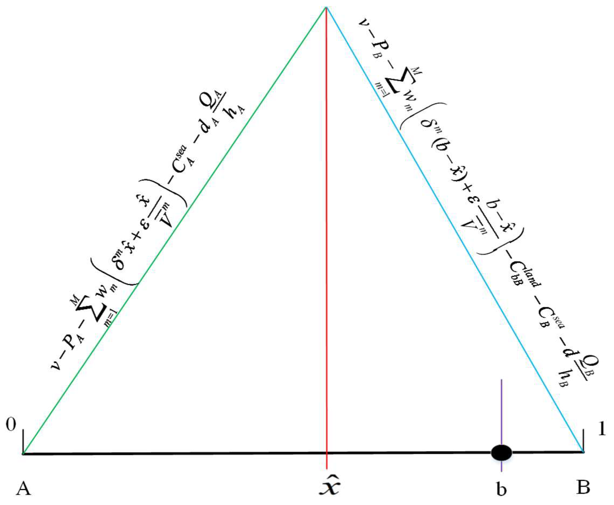
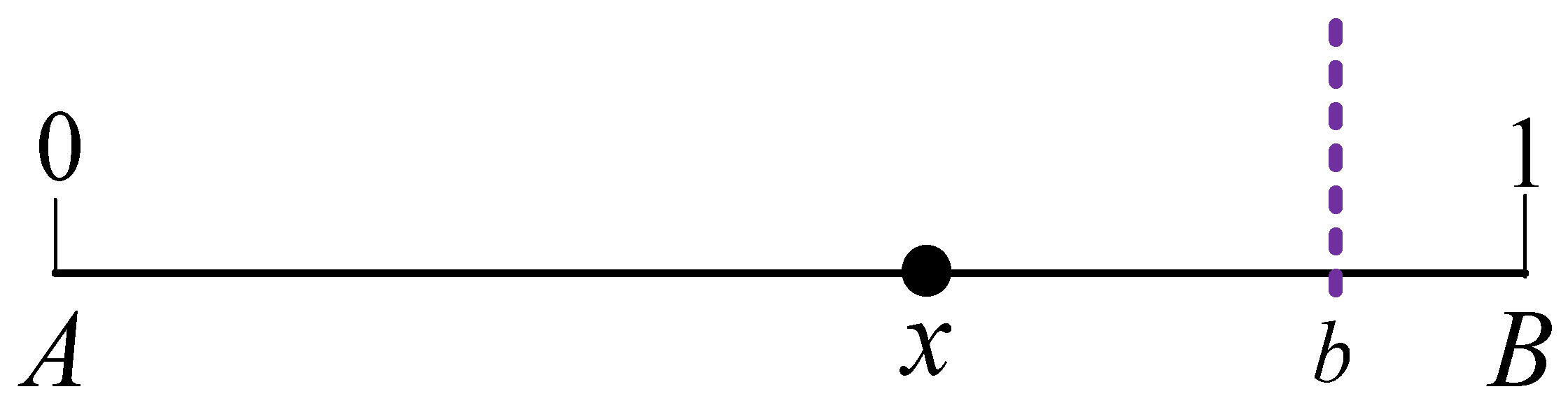
Port: port A and port B are on a line of length 1, at 0 and 1, respectively (see Figure 2). The hinterlands of the two ports overlap, and they are in a competitive state. Both ports can provide the same transshipment loading and unloading services, and their service prices (i.e., port charges to be paid by cargo owners or shippers) are P A and P B , respectively. It is assumed that the port costs (i.e., the costs of transshipment and handling services) provided by port A and port B are C A p o r t and C B p o r t , respectively. The maritime transportation costs (i.e., sea freight to be paid by the cargo owner or shipper) from port A and port B to the overseas destination port K are C A s e a and C B s e a , respectively.
(2)
Cargo owners or shippers: the cargo owner is at a certain point within the [0,1] range, and border port b is located between the cargo owner and port B, that is, 0 < x < b < 1 . Cargo owners and port operators act rationally, making decisions based on their interests and anticipated outcomes. Cargo owners prioritize the most efficient transportation route, while port operators set port service prices to maximize profit or cargo throughput. For simplicity, we assume that cargo demand in the port’s hinterland is inelastic, meaning the demand is constant.
(3)
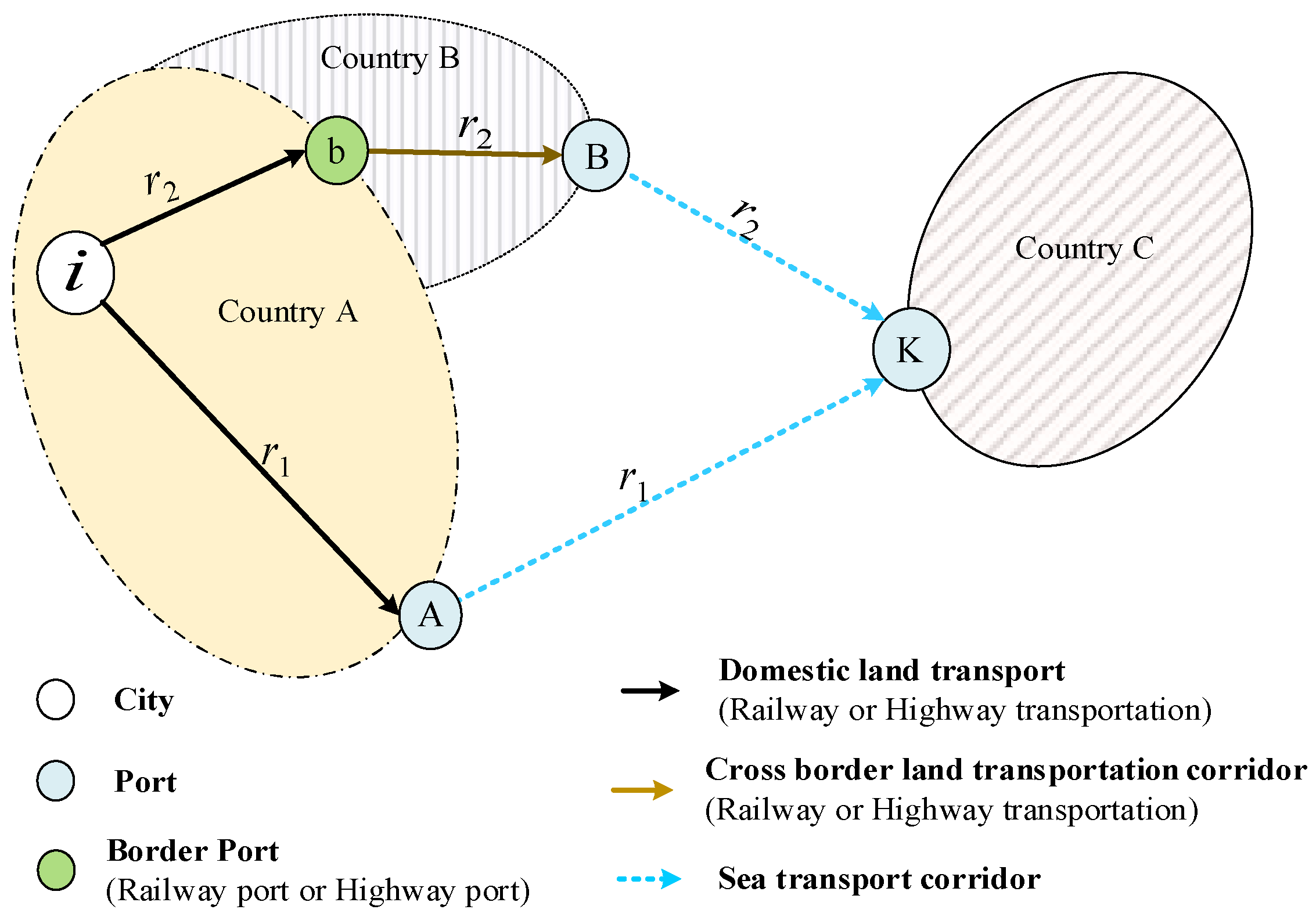
Transportation model: The cargo owner in point x can select port A or port B to transfer the cargo to port K. The land transportation cost of goods from point x to port A is C A land ( x ) , and the land transportation cost of goods from point x to port B is C B l a n d ( x ) = C B l a n d ( b x ) + C b B l a n d , where C B l a n d ( b x ) is the domestic land transportation cost from point x to border port b , and C b B l a n d is the cross-border land transportation cost from border port b to port B.
According to the above assumptions, the utility of transshipment of goods to port K by selecting port A or port B is as follows:
U i ( x ) = U A ( x ) = v P A C A l a n d ( x ) C A s e a d Q A h A U B ( x ) = v P B C B l a n d ( b x ) C b B l a n b C B s e a d Q B h B ,   i = A , B
where U A ( x ) and U B ( x ) represent the direct utility that the cargo owners or shippers at point x choose port A and port B to arrive at destination port K, respectively; v represents the cargo owner’s maximum willingness to pay, assuming that it is large enough to ensure that the effect function is always greater than 0; and P A and P B represent the business pricing for the import and export of containers at port A and port B, respectively (port charges to be paid by the cargo owners or shipper). The transportation cost of importing and exporting goods includes not only transportation expenses, port charges, and sea freight but also negative effects caused by port congestion. In this paper, d Q A h A and d Q B h B , respectively, represent the congestion effect of port A and port B, where d is the marginal cost of port congestion, Q A and Q B , respectively, represent the cargo throughput of port A and port B, and h A and h B , respectively, represent the cargo handling capacity of port A and port B.

2.2. Land Transportation Cost in the Port Hinterland

The cargo owner or shipper at point x can select to arrive at a port by road or railway. In order to better reflect the level of hinterland collection and distribution and port accessibility, this paper uses the weighted comprehensive transportation cost to calculate the land transportation cost as follows:
C A l a n d ( x ) = m = 1 M w m δ m x + ε x V ¯ m
where C A l a n d ( x ) represents the transportation cost from the point x to port A. x represents point x in the interval [0,1], and the shortest distance from it to port A is x ; w m represents the freight sharing rate of the m transport mode; δ m the unit distance transportation cost of the m transport mode; V ¯ m represents the average running speed of the m transport mode; and ε represents the value of time.
Similarly, the cargo at point x can be transported by road or rail to border port b and then be transported to port B by cross-border transportation. The calculation formula of land transportation cost for transportation to port B is as follows:
C B l a n d ( x ) = C x b l a n d + C b B l a n d = m = 1 M w m δ m ( b x ) + ε b x V ¯ m + C b B l a n d
where C B l a n d ( x ) represents the transportation cost from point x to port B. C x b l a n d represents the transportation cost from point x to border port b , and its calculation method is the same as that of C A l a n d ( x ) . C b B l a n d represents the cross-border land transportation cost from border port b to port B.

2.3. Port Cargo Demand

By substituting Equations (2) and (3) into Equation (1), a more specific utility function is obtained as follows:
U i ( x ) = U A ( x ) = v P A m = 1 M w m δ m x + ε x V ¯ m C A s e a d A Q A h A U B ( x ) = v P B m = 1 M w m δ m ( b x ) + ε b x V ¯ m C b B l a n d C B s e a d B Q B h B ,   i = A , B
In the interval [0,1], there must exist a critical point x where the utility of the shipper’s choice of port A and port B for transshipment are equal, that is, there is a point x ( x = x ^ ) that makes U A ( x ^ ) = U B ( x ^ ) .
v P A m = 1 M w m δ m x ^ + ε x ^ V ¯ m C A s e a d A Q A h A = v P B m = 1 M w m δ m ( b x ^ ) + ε b x ^ V ¯ m C b B l a n d C B s e a d Q B h B
To facilitate narration, we replace d h A and d h B by H A and H B , respectively. According to Equation (5), it can be further obtained as follows:
x ^ = P B P A + C B s e a C A s e a + C b B l a n d + b m = 1 M w m δ m + ε 1 V ¯ m + H B Q B H A Q A 2 m = 1 M w m δ m + ε 1 V ¯ m
As shown in Figure 3, when x < x ^ , the transportation cost for selecting port A (green line) is less than the transportation cost for selecting port B (blue line), indicating that the utility of selecting port A to transport goods to port K is greater than that of selecting port B. Consequently, the shipper will prioritize selecting port A for transporting to destination port K. Conversely, when x > x ^ , the transportation cost for selecting port A (green line) is greater than the transportation cost for selecting port B (blue line), and the shipper will prioritize selecting port B for transporting goods to port K. In other words, the critical point x ^ determines the shippers’ choice: those on the left side will select port A, while those on the right side will choose port B.
Since the hinterland of the port is a unit linear space, with port A at position 0, according to the assumption that Q A + Q B = 1, the cargo demand functions of port A and port B under perfect competition mode are as follows:
Q A = P B P A + C B s e a C A s e a + C b B l a n d + b m = 1 M w m δ m + ε 1 V ¯ m + H B 2 m = 1 M w m δ m + ε 1 V ¯ m + H A + H B
Q B = P A P B + C A s e a C B s e a C b B l a n d + ( 2 b ) m = 1 M w m δ m + ε 1 V ¯ m + H A 2 m = 1 M w m δ m + ε 1 V ¯ m + H A + H B
It can be seen in Equations (7) and (8) that the cargo throughput of the two ports is related to each other’s port charges, maritime transportation costs, cross-border land transportation costs, and port congestion costs, that is, port charges, maritime transportation costs, cross-border land transportation costs, and port congestion costs are the control variables affecting port cargo throughput. When any three of them are determined, the port cargo throughput is a monotonic function of the uncontrolled variables ( Q i ( P i , C i k s e a , C b B l a n d , H i ) ).

3. Analysis of Port Competition Mode and Equilibrium Result

The main factor for ports to attract goods is the port service price (i.e., port charges). In this paper, both port A and port B make decisions at the same time and non-cooperatively to maximize their profits and find the Nash equilibrium solution of two types of container service prices. Based on the above analysis, given the port cargo demand function, the profit function of port A and port B can be expressed as follows:
π A = ( p A C A p o r t ) Q A
π B = ( p B C B p o r t ) Q B
Furthermore, we can substitute Equations (7) and (8) into Equations (9) and (10), respectively, to obtain the profits of port A and port B as follows:
π A = ( p A C A p o r t ) P B P A + C B s e a C A s e a + C b B l a n d + b m = 1 M w m δ m + ε 1 V ¯ m + H B 2 m = 1 M w m δ m + ε 1 V ¯ m + H A + H B
π B = ( p B C B p o r t ) P A P B + C A s e a C B s e a C b B l a n d + ( 2 b ) m = 1 M w m δ m + ε 1 V ¯ m + H A 2 m = 1 M w m δ m + ε 1 V ¯ m + H A + H B
In this paper, port A and port B make decisions on the pricing of import and export container services, maritime transportation costs, cross-border land transportation costs, and port cargo handling capacity in the hinterland, and both aim to maximize their own profits in a non-cooperative manner. The objective functions for port A and port B are as follows:
M a x   π A = ( p A C A p o r t ) P B P A + C B s e a C A s e a + C b B l a n d + b m = 1 M w m δ m + ε 1 V ¯ m + H B 2 m = 1 M w m δ m + ε 1 V ¯ m + H A + H B
M a x   π B = ( p B C B p o r t ) P A P B + C A s e a C B s e a C b B l a n d + ( 2 b ) m = 1 M w m δ m + ε 1 V ¯ m + H A 2 m = 1 M w m δ m + ε 1 V ¯ m + H A + H B
By calculating the first-order partial derivatives in Equations (11) and (12) and further simplifying the derivation, the optimal pricing of ports at their respective profit maximization can be obtained as follows (* represents the optimal value in the equilibrium):
P A * = C B s e a C A s e a + C b B l a n d + ( 2 + b ) m = 1 M w m δ m + ε 1 V ¯ m + 2 H B + H A + 2 C A p o r t + C B p o r t 3
P B * = C A s e a C B s e a C b B l a n d + ( 4 b ) m = 1 M w m δ m + ε 1 V ¯ m + 2 H A + H B + 2 C B p o r t + C A p o r t 3
Substituting P A * and P B * into the port demand function, the equilibrium cargo demand for port A and port B can be calculated as follows:
Q A * = C B s e a C A s e a + C b B l a n d + ( 2 + b ) m = 1 M w m δ m + ε 1 V ¯ m + H A + 2 H B + C B p o r t C A p o r t 6 m = 1 M w m δ m + ε 1 V ¯ m + 3 H A + 3 H B
Q B * = C A s e a C B s e a C b B l a n d + ( 4 b ) m = 1 M w m δ m + ε 1 V ¯ m + H B + 2 H A + C A p o r t C B p o r t 6 m = 1 M w m δ m + ε 1 V ¯ m + 3 H A + 3 H B
By substituting the equilibrium cargo demand for port A (Equation (17)) and the optimal pricing of port A (Equation (15)) into Equation (9), the maximum profit function of port A can be obtained as follows:
π A * = C B s e a C A s e a + C b B l a n d + ( 2 + b ) m = 1 M w m δ m + ε 1 V ¯ m + 2 H B + H A + C B p o r t C A p o r t 2 9 2 m = 1 M w m δ m + ε 1 V ¯ m + H A + H B
Likewise, by substituting the equilibrium cargo demand for port A (Equation (18)) and the optimal pricing of port A (Equation (16)) into Equation (10), the maximum profit function of port B can be obtained as follows:
π B * = C A s e a C B s e a C b B l a n d + ( 4 b ) m = 1 M w m δ m + ε 1 V ¯ m + H B + 2 H A + C A p o r t C B p o r t 2 9 ( 2 m = 1 M w m δ m + ε 1 V ¯ m + H A + H B )
Proposition 1.
Compared with port A, the higher the maritime transportation cost of port B and the cross-border land transportation cost of goods transported to port B, the higher the cargo transportation demand and the equilibrium price of port A, and the lower the cargo transportation demand and the equilibrium price of port B, resulting in a decrease in the competitiveness of port B.
Proof. 
By calculating the first-order partial derivative of the optimal pricing and equilibrium cargo demand of port A and port B, that is, P i * C B s e a C A s e a = 0 ,   Q i * C B s e a C A s e a = 0 , P i * C b k l a n d = 0 ,   Q i * C b k l a n d = 0   ( i = A , B ) , the following can be obtained:
P A * C B s e a C A s e a = P A * C b B l a n d = 1 3 > 0 ,   P B * C B s e a C A s e a = P B * C b B l a n d = 1 3 < 0
Q A * C B s e a C A s e a = Q A * C b B l a n d = 1 6 m = 1 M w m δ m + ε 1 V ¯ m + 3 H A + 3 H B > 0 Q B * C B s e a C A s e a = Q B * C b B l a n d = 1 6 m = 1 M w m δ m + ε 1 V ¯ m + 3 H A + 3 H B < 0
This indicates that the equilibrium price and equilibrium demand of port A increase with the increase in C B s e a C A s e a , while the equilibrium price and equilibrium demand of port B decrease with the increase in C B s e a C A s e a . The equilibrium prices and equilibrium demand of port A increase with the increase in C b B l a n d , while the equilibrium price and equilibrium demand of port B decrease with the increase in C b B l a n d . □
The higher the maritime transportation cost of port B and the cost of cross-border land transportation to port B, the more competitive port A will be in terms of transport costs, making it more attractive for cargo. As a result, this would lead to an increase in both the equilibrium price and the demand for port A, while causing a decrease in the equilibrium price and demand for port B. Therefore, even though the area near port B has a proximity advantage, the significant costs associated with cross-border and maritime to port B could reduce its attractiveness to hinterland goods, putting it at a disadvantage in competition with port A.
Proposition 2.
If the sum of the land transport cost, maritime transport cost, and port cost when the shipper selects port B is greater than the sum of the land transport cost, maritime transport cost, and port cost when the shipper selects port A (that is, the total transportation cost when selecting port B is greater than the total transportation cost when choosing port A), then the profit of port A increases with the increase in  C B s e a C A s e a . However, if the total transportation cost for the shipper to select port B is less than the total transportation cost for selecting port A, meaning that selecting port A does not offer a cost advantage over port B for the shipper, then the profit of port A will not increase with the increase in  C B s e a C A s e a .
Proof. 
Taking port A as an example, it can be seen in Equation (19) that π A * is a quadratic function with respect to C B s e a C A s e a . When C B s e a C A s e a ,   C b B l a n d ( 2 + b ) m = 1 M w m δ m + ε 1 V ¯ m 2 H B H A C B p o r t + C A p o r t , π A * decreases as C B s e a C A s e a increases, while when C B s e a C A s e a   C b B l a n d ( 2 + b ) m = 1 M w m δ m + ε 1 V ¯ m 2 H B H A C B p o r t + C A p o r t , + , π A * increases as C B s e a C A s e a increases. □
This indicates that C B s e a C A s e a ,   C b B l a n d ( 2 + b ) m = 1 M w m δ m + ε 1 V ¯ m 2 H B H A C B p o r t + C A p o r t , that is, C B s e a + C B p o r t + m = 1 M w m δ m ( b x ) + ε b x V ¯ m + C b B l a n d + H B C A p o r t + C A s e a + m = 1 M w m δ m x + ε x V ¯ m + H A , although the maritime transportation cost advantage of port A is more obvious with the increase in C B s e a C A s e a , and the total transportation costs to be paid by shippers when they select port B are smaller than the total cost to be paid when they select port A. In this scenario, despite the increase in C B s e a C A s e a , the maritime transportation cost advantage of port A cannot offset the land transport cost advantage of port B, and shippers will still select port B for cargo transportation. Consequently, the demand for goods in port A decreases, and the equilibrium profit of port A decreases with the increase in C B s e a C A s e a .
However, when C B s e a C A s e a   C b B l a n d ( 2 + b ) m = 1 M w m δ m + ε 1 V ¯ m 2 H B H A C B p o r t + C A p o r t , + , that is when C B s e a + C B p o r t + m = 1 M w m δ m ( b x ) + ε b x V ¯ m + C b B l a n d + H B C A p o r t + C A s e a + m = 1 M w m δ m x + ε x V ¯ m + H A , the total transportation costs to be paid by shippers when they select port A are smaller than the total cost to be paid when they select port B. With the increase in C B s e a C A s e a , the maritime transportation cost advantage of port A is much greater than the land transportation cost of port B. Therefore, more shippers select port A for cargo transportation with the increase in C B s e a C A s e a ; the equilibrium demand of port A increases, and the equilibrium price and profit of port A keep increasing.
Proposition 3.
If port A has an advantage in maritime transportation cost and port cost, an increase in cross-border transportation costs of port B will weaken its competitiveness, while the competitiveness and profit of port A will increase. However, if port A has no advantage in both maritime transportation cost and port cost, within a certain range, the profit of port A decreases with the increase in cross-border transportation costs of port B. Only when the cross-border transportation cost of port B is sufficiently high, its disadvantage in port and sea transportation cost can be offset, resulting in an increase in the profit of port A.
Proof. 
It can be seen in Equation (19) that π A * is a quadratic function with respect to C b k l a n d . When C B s e a C A s e a + ( 2 + b ) m = 1 M w m δ m + ε 1 V ¯ m + 2 H B + H A + C B p o r t C A p o r t > 0 , π A * increases with C b k l a n d . When C B s e a C A s e a + ( 2 + b ) m = 1 M w m δ m + ε 1 V ¯ m + 2 H B + H A + C B p o r t C A p o r t < 0 , if C b k l a n d 0 ,   C A s e a C B s e a ( 2 + b ) m = 1 M w m δ m + ε 1 V ¯ m 2 H B H A C B p o r t + C A p o r t , π A * decreases as C b k l a n d increases, and if C b k l a n d   C A s e a C B s e a ( 2 + b ) m = 1 M w m δ m + ε 1 V ¯ m 2 H B H A C B p o r t + C A p o r t , + , π A * increases as C b k l a n d increases. □
This indicates that when port A has advantages in both port cost and maritime transportation cost over port B, meaning the port cost and maritime transportation cost of port A are lower than port B, an increase in cross-border transportation costs to port B will result in higher land transportation costs for port B. Consequently, shippers tend to choose port A, leading to higher demand for port A, stronger competitiveness for port A, and higher profits. However, when port A does not have any advantage in port cost and maritime transportation cost compared to port B, even if the cross-border transportation cost to port B increases, it cannot offset the disadvantage of port A in terms of port cost and maritime transportation cost. Only when the cross-border transportation costs of port B reach a certain level can the land transportation costs of port A become more significant, thus offsetting the disadvantage of port A in port costs and maritime transportation costs, resulting in an increase in the profit of port A with an increase in cross-border transportation costs.

4. Numerical Analysis

This paper conducts a numerical analysis of the hinterland competition between Dalian Port and Vladivostok Port as a case study. Dalian Port is the largest comprehensive foreign trade port in Northeast China, and its total import and export value accounts for nearly three-quarters of the total import and export value in Northeast China. Vladivostok Port is the largest trading port in the Russian Far East and serves as an important two-way transportation hub connecting Asia, Russia, and Europe, with its cargo throughput ranking first in the Russian Far East. With the implementation of the development strategy of the Russian Far East, the cargo throughput of Vladivostok Port has continued to grow rapidly in recent years. Table 1 shows an overview of container terminals of Dalian Port and Vladivostok Port.
However, the Primorsky International Transport Corridor (PITC) has provided a new port option for Northeast China’s foreign trade transportation. Goods for foreign trade transportation from Northeast China can be transported to Vladivostok Port via the PITC and then transshipped to overseas destination ports through Vladivostok Port. Taking Harbin as an example, the new transport route (Harbin–Suifenhe–Vladivostok Port–Busan Port) has the advantage of distance over the traditional transport route (Harbin–Dalian Port–Busan Port) in land transportation, which can significantly shorten transportation time and costs (as shown in Figure 4). It is anticipated that the PITC will enhance port accessibility and cargo circulation efficiency in Northeast China. However, at the same time, it will also intensify the competition between Vladivostok Port and Dalian Port in the Northeast hinterland market.

4.1. Data and Parameters

In this paper, the competitive hinterland of Dalian Port and Vladivostok Port is considered to be the three northeastern provinces of China (Liaoning Province, Jilin Province, and Heilongjiang Province), with a focus on the competition of the two ports in the import and export container market in Northeast China.
In land transportation, m = 1 represents highway transportation and m = 2 represents railway transportation. The freight sharing rate is determined based on the average freight turnover ratio of highways and railways in the three northeastern provinces of China. The container transportation cost of highway transportation is set based on the data released by the Price Monitoring Center of the China Development and Reform Commission (https://www.cfpci.org.cn/Index (accessed on 10 May 2023)), while the container transportation cost of railways is set based on the container transportation price released by China Railway Transport Corporation (http://www.chinainlandport.org.cn/index.php?m=content&c=index&a=show&catid=34&id=169 (accessed on 13 August 2023)). The average operating speeds of highways and railways are set according to the People’s Republic of China Industry Standard (JTGB01-2014): Technical Standard for Highway Engineering and the website data of the China Railway Service Center. Due to the cross-border transportation involving a series of customs clearance operations, such as cargo reloading and customs loading and unloading at border ports, we have set up the cross-border transportation uniformly based on the port charge standards announced by the Suifenhe Railway Port and refer to the railway transportation charges standards for the Russian section of the China Europe Express (http://www.suifenhe.gov.cn/channels/4416.html (accessed on 5 December 2023)).
Regarding port charges, the unit container port charges of Dalian Port and Vladivostok Port shall be set according to the container charge standards published by Dalian Port Container Development Company and FESCO, respectively. The specific model parameters are shown in Table 2.

4.2. Sensitivity Analysis

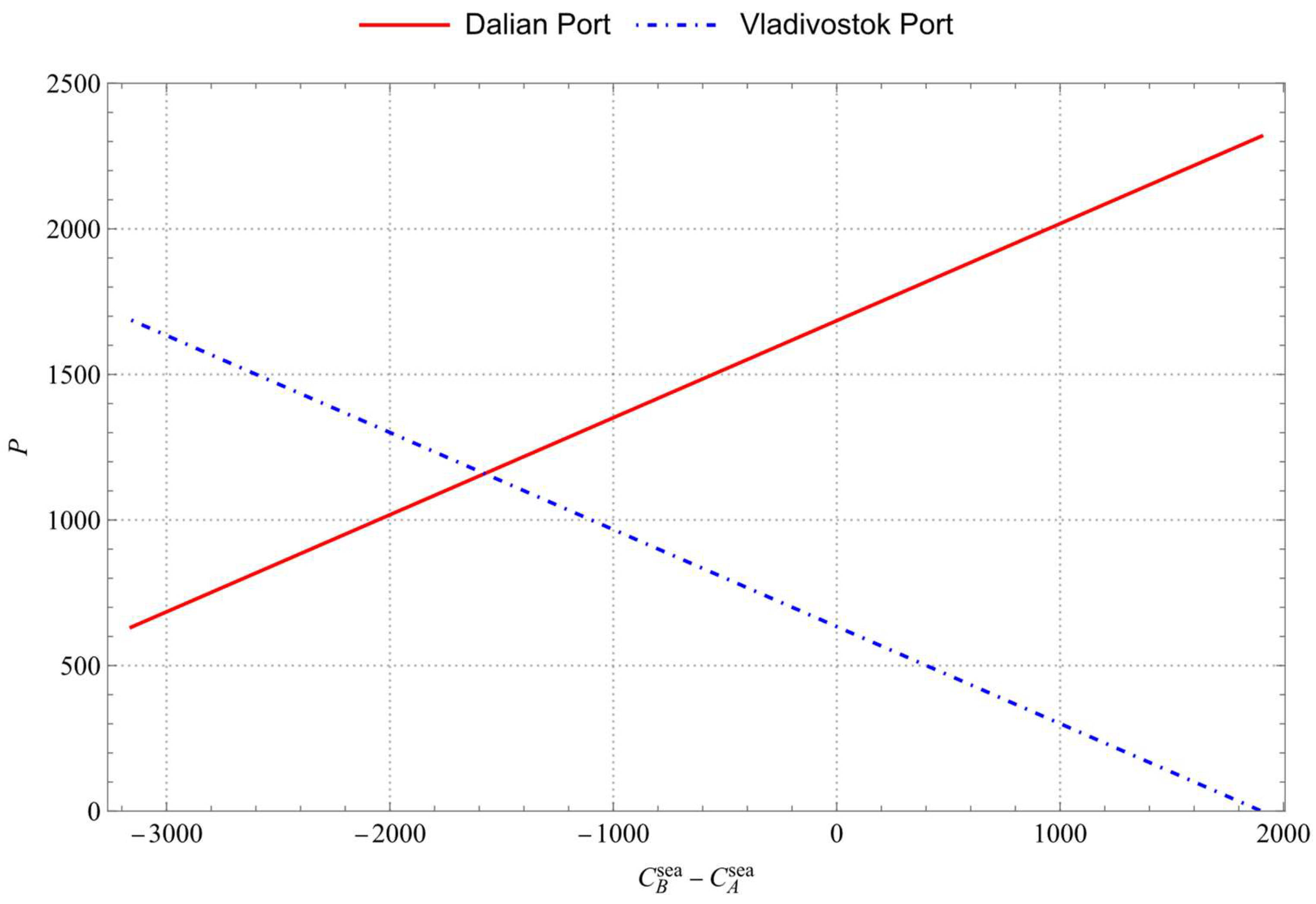
4.2.1. Sensitivity Analysis of Maritime Transportation Cost to Equilibrium Price and Port Cargo Demand

Figure 5 shows the change in port equilibrium price with the maritime transportation cost difference. It can be seen that the equilibrium price of Dalian Port increases with the increase in C B s e a C A s e a , while the equilibrium price of Vladivostok Port decreases with the increase in C B s e a C A s e a . When C B s e a C A s e a = 0 , the maritime transportation costs of Dalian Port and Vladivostok are the same, the equilibrium price of Dalian Port and Vladivostok Port is 1684.57 RMB/TEU and 633.89 RMB/TEU, respectively. When C B s e a C A s e a = 1576.02 RMB/TEU, the maritime transportation cost of Vladivostok Port can save 1576.02 RMB/TEU compared with that of Dalian Port, and then the equilibrium price of Vladivostok Port and Dalian Port is the same. When C B s e a C A s e a < 1576.02 RMB/TEU, the equilibrium price of Vladivostok Port is greater than that of Dalian Port; when C B s e a C A s e a > 1576.02 RMB/TEU, the equilibrium price of Vladivostok Port is less than that of Dalian Port.
Figure 6 shows the change in the maritime transportation cost difference on port equilibrium cargo demand. It can be seen that the equilibrium cargo demand of Dalian Port increases with the increase in C B s e a C A s e a , while the equilibrium cargo demand of Vladivostok Port decreases with the increase in C B s e a C A s e a . When C B s e a C A s e a = 3023.02 RMB/TEU, that is, when Vladivostok Port can save 3023.02 RMB in maritime transportation costs compared with Dalian Port, the equilibrium cargo demand of Vladivostok Port and Dalian Port is the same, and Vladivostok Port will share the market in the hinterland of Northeast China equally with Dalian port. When C B s e a C A s e a < 3023.02 RMB/TEU, the equilibrium cargo demand of Vladivostok Port will exceed that of Dalian Port; When C B s e a C A s e a > 3023.02 RMB/TEU, the equilibrium cargo demand of Vladivostok Port will exceed that of Dalian Port; the equilibrium cargo demand of Vladivostok Port will be smaller than of Dalian port.
In addition, it can be observed that C B s e a C A s e a decreased from −2993.32 RMB/TEU to −3052.72 RMB/TEU, and the demand for Vladivostok Port decreased from 100% to 0. If factors such as land transportation costs, cross-border transportation costs, and port costs remain unchanged, and the maritime transportation cost of Vladivostok Port is reduced from 2993.32 RMB/TEU to 3052.72 RMB/TEU, it would make Vladivostok Port competitive. Within this range, the reduction in the maritime transportation cost would significantly increase the market share of the hinterland of Vladivostok Port.

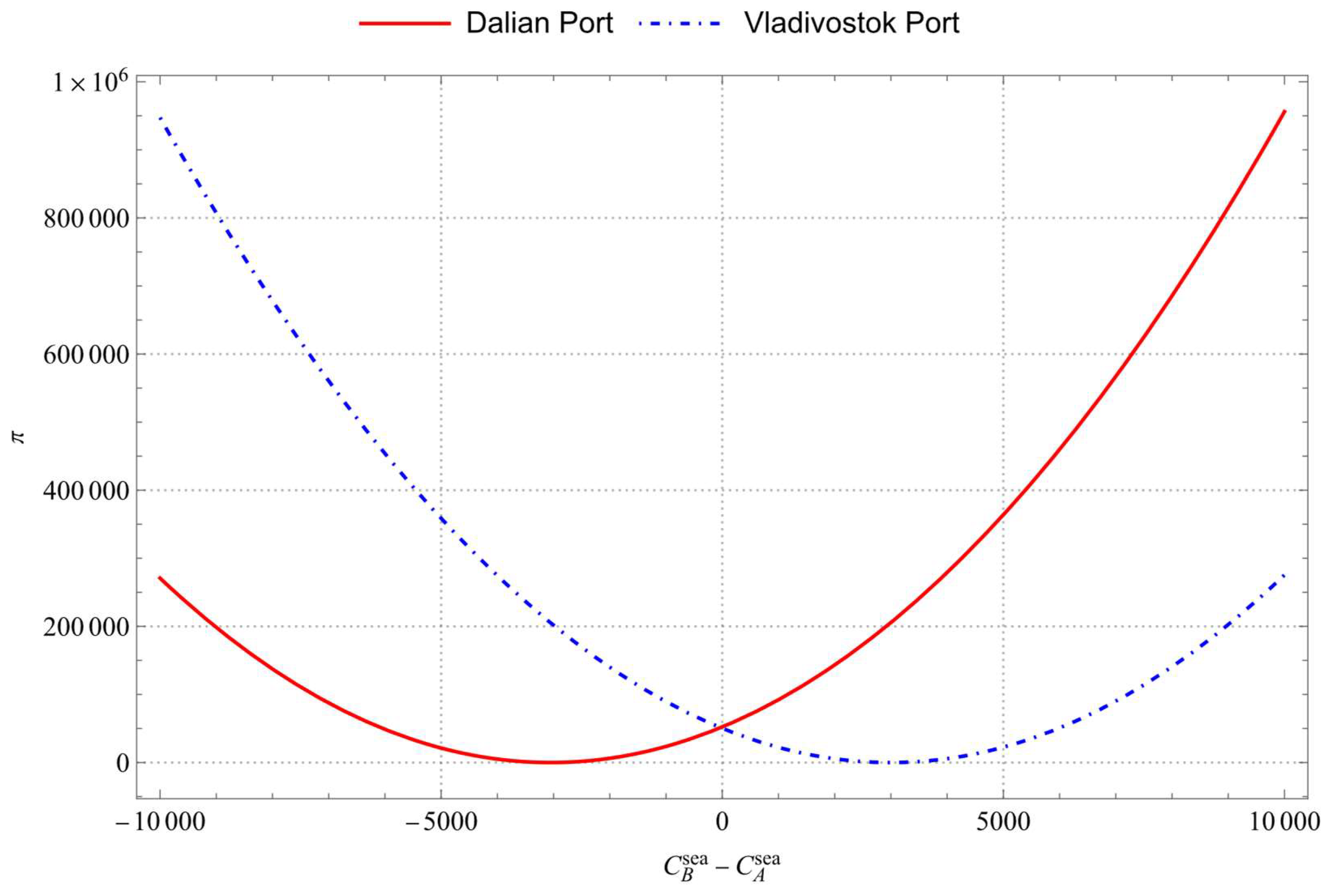
4.2.2. Sensitivity Analysis of Maritime Transportation Cost to Port Equilibrium Profit

Figure 7 shows the change in the maritime transportation cost difference on port equilibrium profit. It can be seen that when C B s e a C A s e a = 3052.72 RMB/TEU, Dalian Port has the lowest profit. When C B s e a C A s e a > 3052.72 RMB/TEU, the profit of Dalian Port increases with the increase in C B s e a C A s e a , while when C B s e a C A s e a < 3052.72 RMB/TEU, Dalian Port’s profit decreases with the increase in C B s e a C A s e a . Meanwhile, when C B s e a C A s e a = 2993.32 RMB/TEU, Vladivostok Port has the lowest profit. When C B s e a C A s e a > 2993.32 RMB/TEU, the profit of Vladivostok Port increases with the increase in C B s e a C A s e a , while when C B s e a C A s e a < 2993.32 RMB/TEU, the profit of Vladivostok Port decreases with the increase in C B s e a C A s e a .
In addition, when C B s e a C A s e a < 29.7 RMB/TEU, the profit of Vladivostok Port will exceed that of Dalian Port, and when C B s e a C A s e a > 29.7 RMB/TEU, the profit of Dalian Port will exceed that of Vladivostok Port. This means that only if the maritime transportation cost of Vladivostok Port can save −29.7 RMB/TEU compared with Dalian Port, its profit can exceed Dalian Port.

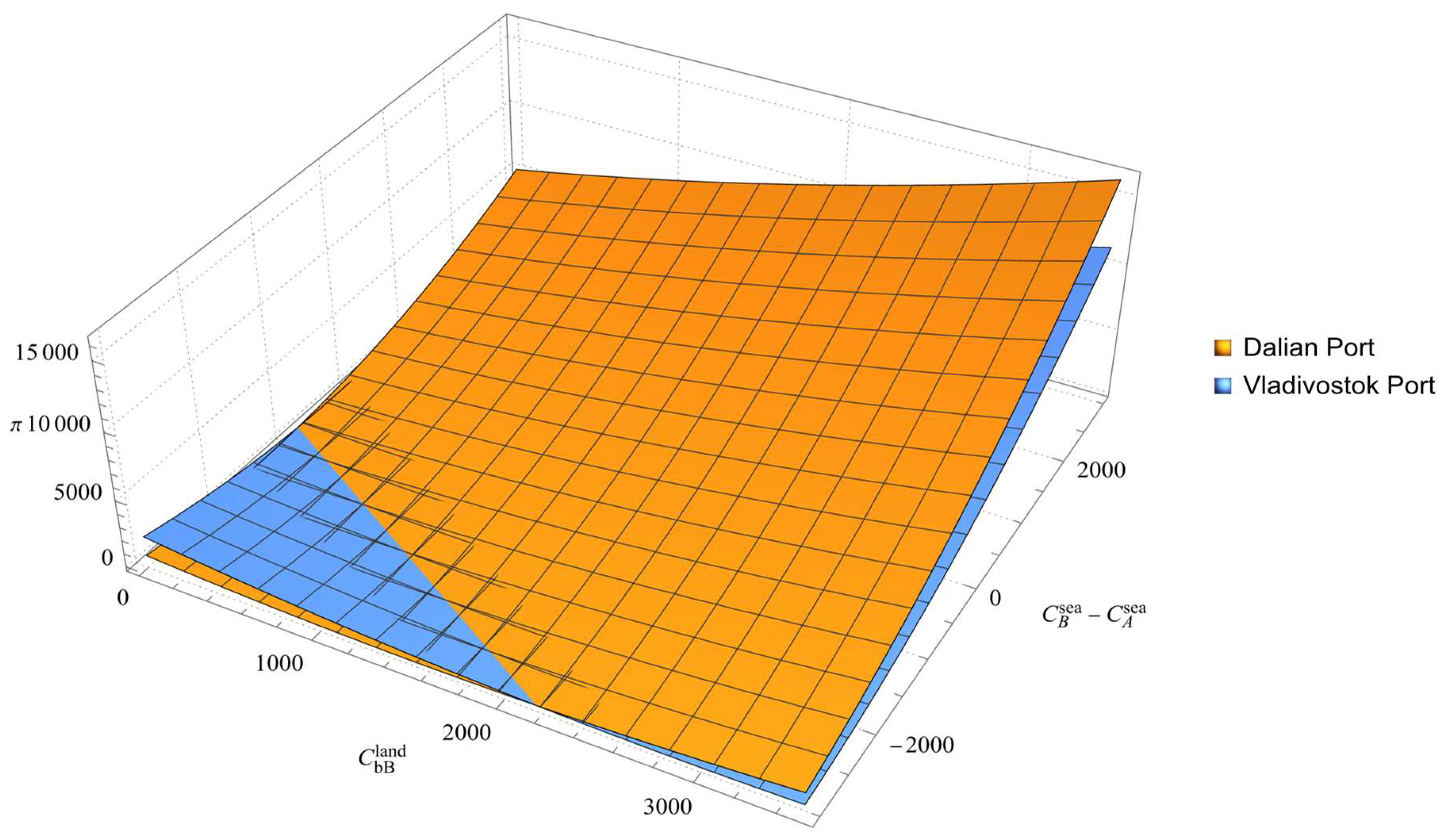
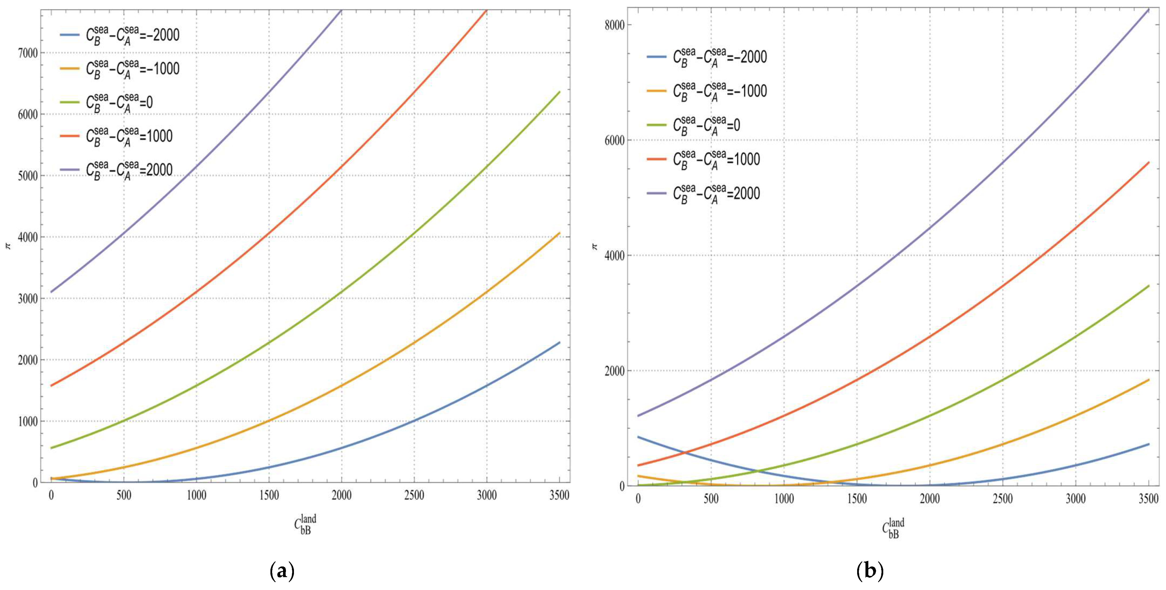
4.2.3. Sensitivity Analysis of Cross-Border Land transportation Cost and Maritime Transportation Cost to Port Equilibrium Profit

Figure 8 shows the port equilibrium profit as the cross-border transportation cost and maritime transportation cost difference. It can be seen that on the whole, with the simultaneous increase in C b B l a n d and C B s e a C A s e a , the profits of Dalian Port and Vladivostok Port also increase, and the profit of Dalian Port increases faster than that of Vladivostok Port. However, when C b B l a n d and C B s e a C A s e a decline at the same time, the profit of Dalian Port declines faster than that of Vladivostok Port. When C b B l a n d and C B s e a C A s e a decline to a certain extent at the same time, the profit of Dalian Port will be less than that of Vladivostok Port to a certain extent. When the cost of cross-border transportation to Vladivostok Port is higher, and the maritime transportation cost of Vladivostok Port is higher than that of Dalian Port, the cost for shippers to choose Vladivostok Port for cargo transportation will increase. The substitution between Vladivostok Port and Dalian Port will decrease, and the monopoly ability of the two ports to nearby shippers will be enhanced, so the profits of the two ports also increase.
Figure 9a illustrates the cross-sectional view of profit change for Dalian Port in Figure 8, considering various C B s e a C A s e a : −2000 RMB/TEU, −1000 RMB/TEU, 0 RMB/TEU, 1000 RMB/TEU, and 2000 RMB/TEU. It can be seen that the profit of Dalian Port increases with the increase in C b B l a n d , and the larger the value of C B s e a C A s e a , the greater the profit growth of Dalian Port. Figure 9b illustrates the cross-sectional view of profit change for Vladivostok Port in Figure 8, considering various C B s e a C A s e a : −2000 RMB/TEU, −1000 RMB/TEU, 0 RMB/TEU, 1000 RMB/TEU, and 2000 RMB/TEU. It can be seen that when C B s e a C A s e a is negative ( C B s e a C A s e a = −2000 RMB/TEU, −1000 RMB/TEU), the profit of Vladivostok Port decreases first and then increases with the increase in C b B l a n d . When C B s e a C A s e a 0 ( C B s e a C A s e a = 0 RMB/TEU, 2000 RMB/TEU, 1000 RMB/TEU), the profit of Vladivostok Port increases with the increase in C b B l a n d . This means that when the maritime transportation cost of Vladivostok Port has an advantage over Dalian Port (i.e., C B s e a C A s e a < 0 ), the profit of Vladivostok Port will reach a valley within a certain range of cross-border transportation costs.
The results of the numerical simulation show that under the conditions of the PITC, Vladivostok Port will only have a market advantage over Dalian Port in maritime transportation costs if it can save 2993.32 RMB/TEU to 3052.72 RMB/TEU. This means that under the current cross-border transportation conditions, Vladivostok Port should expand its market at the maritime transportation cost of 2993.32 RMB/TEU to 3052.72 RMB/TEU to be profitable. Under the current transportation conditions, if the maritime transportation cost saved by Vladivostok Port is 3052.72 RMB/TEU compared with Dalian Port, then the profit of Dalian Port is the smallest. Dalian Port should avoid competing in the market with Vladivostok Port where the difference in maritime transportation cost is close to 3052.72 RMB/TEU.
A comparison of shipping costs from Dalian and Vladivostok Ports to various ports, including Japanese, Korean, and Chinese coastal ports (As shown in Table 3), reveals that only the Vladivostok Port–Buan Port shipping route has a cost advantage. However, under the current situation of land transportation cost, cross-border transportation cost, port cost, and other factors remain unchanged, Vladivostok–Buan relative to Dalian–Buan saves 352.34 RMB/TEU, which is far less than the range of equilibrium demand for goods. In other words, under the current transportation conditions, the current Vladivostok–Busan shipping rates are not attractive for Northeast cargo. In the route from Vladivostok Port to China’s coastal ports, we use container liner tariffs published by FESCO (https://www.fesco.ru/ru/ (accessed on 2 January 2024)), while the data of ocean freight rates from Dalian to China’s coastal ports come from China’s domestic container tariffs (https://www.epanasia.com/ (accessed on 2 January 2024)). Obviously, there are obvious differences in customs clearance procedures and transportation objects between foreign trade container transportation and domestic trade container transportation. However, for shippers, the advantages of using the PITC transport corridor and Vladivostok Port for transportation are not sufficient. Therefore, if Vladivostok Port wants to capitalize on the Northeast cargo transportation market, it needs to enhance cooperation with China and other neighboring countries, optimize ship types, increase container capacity, reduce PITC transportation costs, or avail relevant transportation subsidies.
Our aim is to assess the impact of the new international land–sea transport corridor on port selection by shippers and analyze how transportation costs affect port container pricing, throughput, and overall profitability. However, in reality, ports may be affected by factors such as severe weather and environmental conditions, which can reduce port operating efficiency and increase costs, which, in turn, affect the overall competitiveness of ports. Although the assumptions in this article are based on the standard setting of the Hotelling model and have been appropriately adjusted in the context of port competition, they may not fully capture the complexity and dynamics of ports in the real world. Thus, conducting a sensitivity analysis of environmental factors to determine the impact of cross-border transportation corridor construction on the competition of neighboring countries’ ports will be an important area for future empirical analysis. In addition, changes in the international political situation may lead to adjustments in port policies and regulations in relevant countries. These adjustments may involve tariffs, trade barriers, import and export restrictions, etc., directly affecting the port’s cargo throughput and international competitiveness. Therefore, in future research, it is necessary to further consider these factors and better simulate and analyze the impact of the new land–sea intermodal corridor on the oligarchic port competition of neighboring countries.

5. Conclusions

Utilizing the Hotelling model and considering the influence of comprehensive transportation costs on shippers’ port selection, this paper explores the impact of cross-border transportation corridor construction on ports between neighboring countries. Additionally, this study examines the effect of the Primorsky International Transport Corridor (PITC) on the competition between Dalian Port and Vladivostok Port, analyzing how cross-border transportation costs and shipping costs influence the pricing of port containers, container cargo throughput, profit, and related issues.
Based on the model derivation and numerical analysis, the following main conclusions are drawn:
(1)
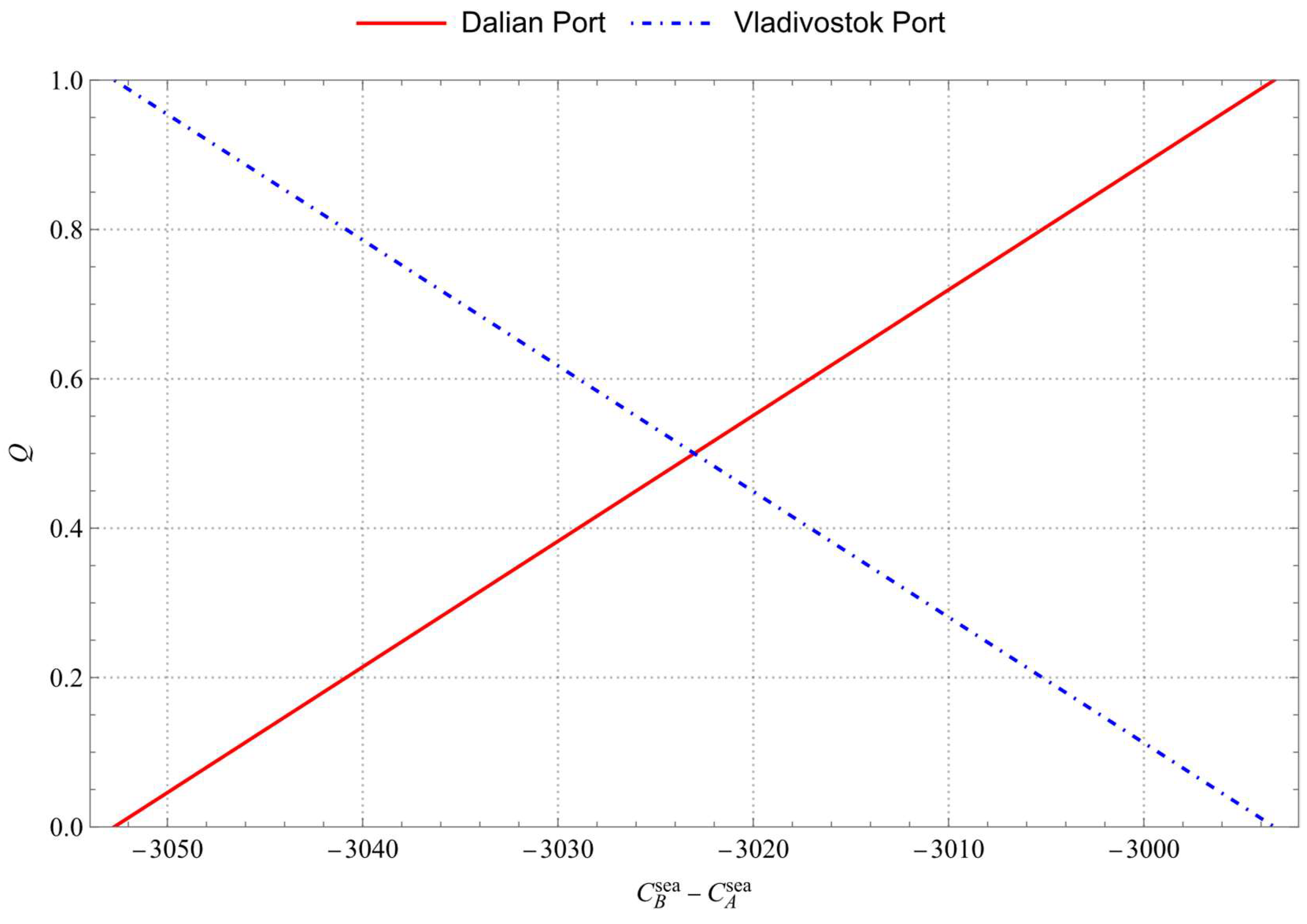
The higher the cross-border land transportation cost of goods transported to the overseas port and the maritime transportation cost of goods transported from the overseas port to the destination port, the lower the demand and price of goods of the overseas port in this region, putting it at a disadvantage compared to the port in this region. It is worth mentioning that the operational efficiency and capacity of the new international land–sea transport corridor would also be affected by international politics, geopolitics, market environment, and other factors, so the operational efficiency and cost of the international land–sea transport corridor is one of the important factors that restrict the expansion of overseas ports to the hinterland of the region.
(2)
In the case that overseas ports have a cost disadvantage compared with domestic ports when their maritime transportation cost is higher, the profit increase in domestic ports will be greater. Conversely, if overseas ports have a cost advantage over domestic ports, even if their maritime transportation cost is higher, the profit of domestic ports will decrease accordingly.
(3)
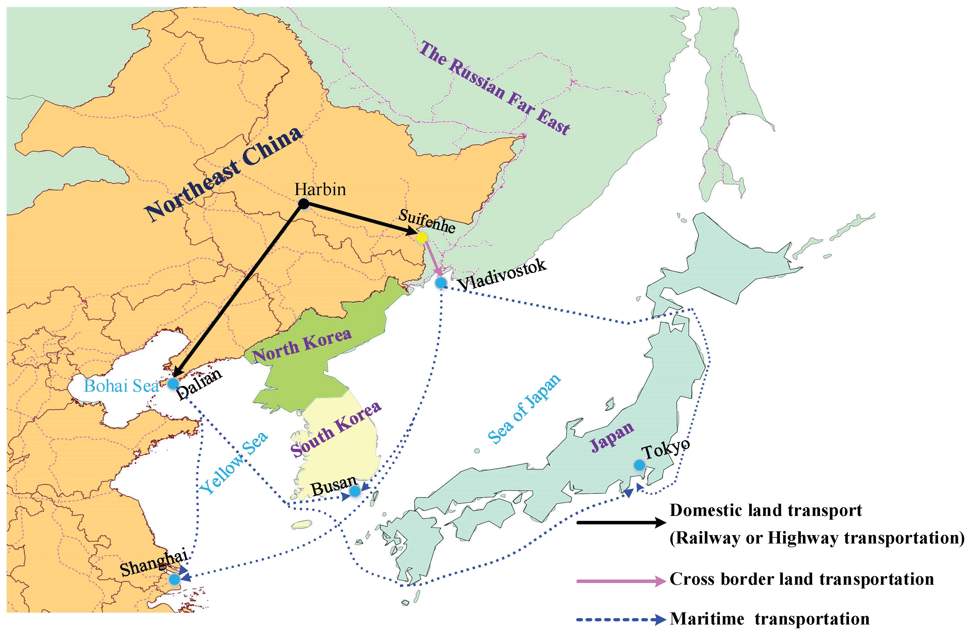
When the overseas port has an advantage in maritime transportation costs, an increase in cross-border transportation costs can enhance its competitiveness. Conversely, when there is no such advantage, cross-border transport costs need to be large enough to offset the disadvantage and thereby increase profits. Given the current conditions of the PITC, high cross-border transportation costs are not conducive to improving the competition of Vladivostok Port in the transportation market of Northeast China. Therefore, further reducing the cross-border transportation cost of the PITC is an important factor to expand the market scope of Vladivostok Port and maintain its profits.

Author Contributions

Conceptualization, C.L. and H.F. (Houming Fan); methodology, C.L. and H.M.; software, C.L.; validation, C.L., H.M. and H.F. (Hao Fan); formal analysis, X.Z.; investigation, H.F. (Hao Fan); resources, H.F. (Houming Fan); data curation, C.L.; writing—original draft preparation, C.L.; writing—review and editing, H.F. (Hao Fan) and H.M.; visualization, X.Z.; supervision, C.L.; project administration, H.F. (Houming Fan); funding acquisition, H.F. (Houming Fan). All authors have read and agreed to the published version of the manuscript.

Funding

This research was funded by the National Social Science Foundation of China (23FGLA010), the Major project of the Social Science Planning Fund of Liaoning Province (L22ZD014), and the National Natural Science Foundation of China (61473053).

Institutional Review Board Statement

Not applicable.

Informed Consent Statement

Not applicable.

Data Availability Statement

The data presented in this study are available upon request from the corresponding author. The data are not publicly available due to privacy concerns.

Acknowledgments

The authors gratefully acknowledge the reviewers for their comments to improve the quality of this paper and would also like to thank the editors for their help with this paper.

Conflicts of Interest

The authors declare no conflicts of interest.

References

  1. Hoffman, A.J. Optimized Border System for Land-Based Transport. IEEE Intell. Transp. Syst. Mag. 2023, 15, 6–21. [Google Scholar] [CrossRef]
  2. Liu, C.; Fan, H.; Zhang, X.; Fan, H.; Miao, H. Impact of the Primorsky International Transport Corridor on the Hinterland Competition between Ports in Northeast China and Russian Far East. Res. Transp. Bus. Manag. 2024, 52, 101084. [Google Scholar] [CrossRef]
  3. Jiang, Y.; Qiao, G.; Lu, J. Impacts of the New International Land–Sea Trade Corridor on the Freight Transport Structure in China, Central Asia, the ASEAN Countries and the EU. Res. Transp. Bus. Manag. 2020, 35, 100419. [Google Scholar] [CrossRef]
  4. Luo, M.; Chen, F.; Zhang, J. Relationships among Port Competition, Cooperation and Competitiveness: A Literature Review. Transp. Policy 2022, 118, 1–9. [Google Scholar] [CrossRef]
  5. Lagoudis, I.N.; Theotokas, I.; Broumas, D. A Literature Review of Port Competition Research. Int. J. Shipp. Transp. Logist. 2017, 9, 724–762. [Google Scholar] [CrossRef]
  6. Huybrechts, M.; Meersman, H.; Van de Voorde, E.; Van Hooydonk, E.; Verbeke, A.; Winkelmans, W. Port Competitiveness: An Economic and Legal Analysis of the Factors Determining the Competitiveness of Seaports; De Boeck: Antwerpen, Belgium, 2002. [Google Scholar]
  7. Huang, Z.; Yang, Y.; Zhang, F. Configuration Analysis of Factors Influencing Port Competitiveness of Hinterland Cities under TOE Framework: Evidence from China. J. Mar. Sci. Eng. 2022, 10, 1558. [Google Scholar] [CrossRef]
  8. Dong, G.; Huang, R. Inter-Port Price Competition in a Multi-Port Gateway Region. Res. Transp. Econ. 2022, 94, 101178. [Google Scholar] [CrossRef]
  9. Yu, S.; Gong, L.; Qi, M. Efficiency Analysis of the Coastal Port Group in the Yangtze River Delta. J. Mar. Sci. Eng. 2022, 10, 1575. [Google Scholar] [CrossRef]
  10. Chang, Y.T.; Talley, W.K. Port Competitiveness, Efficiency, and Supply Chains: A Literature Review. Transp. J. 2019, 58, 1–20. [Google Scholar] [CrossRef]
  11. Parola, F.; Risitano, M.; Ferretti, M.; Panetti, E. The Drivers of Port Competitiveness: A Critical Review. Transp. Rev. 2017, 37, 116–138. [Google Scholar] [CrossRef]
  12. Wang, J.; Mo, L.L.; Ma, Z. Evaluation of Port Competitiveness along China’s “Belt and Road” Based on the Entropy-TOPSIS Method. Sci. Rep. 2023, 13, 15717. [Google Scholar] [CrossRef]
  13. Zhong, H.L.; Ou, Y.H.; Chen, J.W.; Wan, Y.C. Empirical Study on Sustainable Competitiveness Evaluation of Guangzhou Port Based on Improved Matter-Element Model. In Proceedings of the 2017 International Conference on Service Systems and Service Management, Dalian, China, 16–18 June 2017. [Google Scholar]
  14. Wang, P.; Hu, Q.Y.; Xu, Y.J.; Mei, Q.; Wang, F. Evaluation Methods of Port Dominance: A Critical Review. Ocean Coast. Manag. 2021, 215, 105954. [Google Scholar] [CrossRef]
  15. Ren, J.Z.; Dong, L.; Sun, L. Competitiveness Prioritisation of Container Ports in Asia under the Background of China’s Belt and Road Initiative. Transp. Rev. 2018, 38, 436–456. [Google Scholar] [CrossRef]
  16. Li, Z.; Wang, X.; Zheng, R.; Na, S.; Liu, C. Evaluation Analysis of the Operational Efficiency and Total Factor Productivity of Container Terminals in China. Sustainability 2022, 14, 13007. [Google Scholar] [CrossRef]
  17. Lozano, S. Estimating Productivity Growth of Spanish Ports Using a Non-Radial, Non-Oriented Malmquist Index. Int. J. Shipp. Transp. Logist. 2009, 1, 227–248. [Google Scholar] [CrossRef]
  18. Ben Mabrouk, M.; Elmsalmi, M.; Aljuaid, A.M.; Hachicha, W.; Hammami, S. Joined Efficiency and Productivity Evaluation of Tunisian Commercial Seaports Using DEA-Based Approaches. J. Mar. Sci. Eng. 2022, 10, 626. [Google Scholar] [CrossRef]
  19. Yap, W.Y.; Lam, J.S.L. Competition Dynamics between Container Ports in East Asia. Transp. Res. Part A-Policy Pract. 2006, 40, 35–51. [Google Scholar] [CrossRef]
  20. Dias, J.C.Q.; Azevedo, S.G.; Ferreira, J.; Palma, S.F. A Comparative Benchmarking Analysis of Main Iberian Container Terminals: A DEA Approach. Int. J. Shipp. Transp. Logist. 2009, 1, 260–275. [Google Scholar] [CrossRef]
  21. Li, H.; Jiang, L.L.; Liu, J.N.; Su, D.D. Research on the Evaluation of Logistics Efficiency in Chinese Coastal Ports Based on the Four-Stage DEA Model. J. Mar. Sci. Eng. 2022, 10, 1147. [Google Scholar] [CrossRef]
  22. Yen, B.T.H.; Huang, M.-J.; Lai, H.-J.; Cho, H.-H.; Huang, Y.-L. How Smart Port Design Influences Port Efficiency—A DEA-Tobit Approach. Res. Transp. Bus. Manag. 2023, 46, 100862. [Google Scholar] [CrossRef]
  23. Svanberg, M.; Holm, H.; Cullinane, K. Assessing the Impact of Disruptive Events on Port Performance and Choice: The Case of Gothenburg. J. Mar. Sci. Eng. 2021, 9, 145. [Google Scholar] [CrossRef]
  24. De Langen, P.W.; Heij, C. Corporatisation and Performance: A Literature Review and an Analysis of the Performance Effects of the Corporatisation of Port of Rotterdam Authority. Transp. Rev. 2014, 34, 396–414. [Google Scholar] [CrossRef]
  25. Borges Vieira, G.B.; Kliemann Neto, F.J.; Amaral, F.G. Governance, Governance Models and Port Performance: A Systematic Review. Transp. Rev. 2014, 34, 645–662. [Google Scholar] [CrossRef]
  26. Garcia-Alonso, L.; Sanchez-Soriano, J. Port Selection from a Hinterland Perspective. Marit. Econ. Logist. 2009, 11, 260–269. [Google Scholar] [CrossRef]
  27. Lin, Y.; Wang, X. Port Selection Based on Customer Questionnaire: A Case Study of German Port Selection. Eur. Transp. Res. Rev. 2019, 11, 48. [Google Scholar] [CrossRef]
  28. Feng, H.; Lin, Q.; Zhang, X.; Lam, J.S.L.; Yap, W.Y. Port Selection by Container Ships: A Big AIS Data Analytics Approach. Res. Transp. Bus. Manag. 2024, 52, 101066. [Google Scholar] [CrossRef]
  29. Pujats, K.; Golias, M.; Konur, D. A Review of Game Theory Applications for Seaport Cooperation and Competition. J. Mar. Sci. Eng. 2020, 8, 100. [Google Scholar] [CrossRef]
  30. Verhoeff, J.M. Seaport Competition: Some Fundamental and Political Aspects. Marit. Policy Manag. 1981, 8, 49–60. [Google Scholar] [CrossRef]
  31. Yu, M.; Shan, J.; Ma, L. Regional Container Port Competition in a Dual Gateway-Port System. J. Syst. Sci. Syst. Eng. 2016, 25, 491–514. [Google Scholar] [CrossRef]
  32. van Reeven, P. The Effect of Competition on Economic Rents in Seaports. J. Transp. Econ. Policy 2010, 44, 79–92. [Google Scholar]
  33. Yip, T.L.; Liu, J.J.; Fu, X.; Feng, J. Modeling the Effects of Competition on Seaport Terminal Awarding. Transp. Policy 2014, 35, 341–349. [Google Scholar] [CrossRef]
  34. Cui, H.; Notteboom, T. Modelling Emission Control Taxes in Port Areas and Port Privatization Levels in Port Competition and Co-Operation Sub-Games. Transp. Res. Part D Transp. Environ. 2017, 56, 110–128. [Google Scholar] [CrossRef]
  35. Czerny, A.; Höffler, F.; Mun, S. Hub Port Competition and Welfare Effects of Strategic Privatization. Econ. Transp. 2014, 3, 211–220. [Google Scholar] [CrossRef]
Figure 1. The alternative land–sea transportation routes for shippers.
Applsci 14 01857 g001
Figure 2. The hinterland market division of two adjacent ports.
Applsci 14 01857 g002
Figure 3. Hinterland division of port A and port B.
Applsci 14 01857 g003
Figure 4. International land–sea transport routes from cities in Northeast China to overseas destination ports (Harbin to Busan Port as an example).
Applsci 14 01857 g004
Figure 5. The change in port equilibrium price with the maritime transportation cost difference.
Applsci 14 01857 g005
Figure 6. The change in port equilibrium cargo demand with the maritime transportation cost difference.
Applsci 14 01857 g006
Figure 7. The change in port equilibrium profit with the maritime transportation cost difference.
Applsci 14 01857 g007
Figure 8. The change in port equilibrium profit with the cross-border transportation cost and maritime transportation cost difference.
Applsci 14 01857 g008
Figure 9. The change in port equilibrium profit with the cross-border land transportation cost: (a) the change in the profit of Dalian Port with C b B l a n d ; (b) the change in the profit of Vladivostok Port with C b B l a n d .
Applsci 14 01857 g009
Table 1. Overview of container terminals of Dalian Port and Vladivostok Port.
Dalian ProtVladivostok Port
Number of container terminals126
Number of berths at container terminals1810
Number of bridge cranes3514
Container yard area (million square meters)2.931.2
Container cargo throughput (million TEU)445.976.8
Table 2. The setting of model parameters.
ParameterValue
Freight sharing rate w m w 1 = 0.35 , w 2 = 0.65
Transportation cost per unit distance δ m (RMB/TEU·km) δ 1 = 3.18 , δ 2 = 9.185
Average operating speed V ¯ m (km/h) V ¯ 1 = 80 , V ¯ 2 = 90
Cross-border transportation cost C b B l a n d (RMB) C b B l a n d = 2102
Port charge C i p o r t (RMB/TEU) C A p o r t = 667, C B p o r t = 1590
Time value ε (RMB/TEU) ε = 40
Marginal congestion cost of port d (RMB/TEU) d = 0.1
Container cargo handling capacity h i (TEU) h A = 300 , h B = 80
Table 3. Comparison of the cost of maritime transportation routes.
Shipping RouteDirectionMaritime Transportation Cost *
(Ocean Freight)
Maritime Transportation Cost Difference
( C B s e a C A s e a )
Shipping routes to Japanese and Korean portsDalian–Buan2783.45−352.34
Vladivostok–Buan2431.11
Dalian–Tokoy2818.68563.74
Vladivostok–Tokoy3382.42
Shipping routes to Chinese coastal portsDalian–Shanghai1674.001109.45
Vladivostok–Shanghai2783.45
Dalian–Xiamen1464.002376.45
Vladivostok–Xiamen3840.45
Dalian–Nansha1335.002505.45
Vladivostok–Nansha3840.45
* Transportation costs are calculated in RMB.
Disclaimer/Publisher’s Note: The statements, opinions and data contained in all publications are solely those of the individual author(s) and contributor(s) and not of MDPI and/or the editor(s). MDPI and/or the editor(s) disclaim responsibility for any injury to people or property resulting from any ideas, methods, instructions or products referred to in the content.

