Abstract
Machine learning (ML) has become more prevalent as a tool used for biogeochemical analysis in agricultural management. However, a common drawback of ML models is the lack of interpretability, as they are black boxes that provide little insight into agricultural management. To overcome this limitation, we compared three tree-based models (decision tree, random forest, and gradient boosting) to explain soil organic matter content through Shapley additive explanations (SHAP). Here, we used nationwide data on field crops, soil, terrain, and climate across South Korea (n = 9584). Using the SHAP method, we identified common primary controls of the models, for example, regions with precipitation levels above 1400 mm and exchangeable potassium levels exceeding 1 cmol+ kg−1, which favor enhanced organic matter in the soil. Different models identified different impacts of macronutrients on the organic matter content in the soil. The SHAP method is practical for assessing whether different ML models yield consistent findings in addressing these inquiries. Increasing the explainability of these models means determining essential variables related to soil organic matter management and understanding their associations for specific instances.
1. Introduction
Machine learning (ML) has emerged as a crucial domain in science and technology, exerting a substantial socioeconomic–environmental influence on various aspects of human and natural systems [1,2]. ML allows us to learn from vast amounts of data and improve the predictive performance of models. However, ML often employs complex algorithms, which results in black box models due to their intricate internal processes that are not readily interpretable [3,4,5]. Such opaqueness may lead stakeholders to overlook meaningful patterns or issues arising from hidden biases in the data. This hinders the handling of effective predictive resource management, mainly when based on large-scale ML [6]. For example, the accuracy problem of yield mapping is well-known due to errors inherent in high data volumes and algorithm opacity [7].
Considerable concern has been expressed about relying on opaque models that may result in decisions that are not fully comprehended or, even worse, violate ethical principles regarding business and the environment or legal norms [1,8]. These risks are particularly relevant for decision-making in real-life scenarios and for access to public benefits [9], for example, digitalization in agriculture [10] and terrestrial conservation [11]. This partly explains the low adoption rate of current ML-based decision support systems in many areas. Land managers, government agencies, and companies that incorporate black box ML models into their practices, products, and applications potentially face efficiency, safety, and trust issues [12]. Therefore, the lack of interpretability must be addressed, and increasing the explainability of predictive modeling for data analysis is becoming increasingly important for mitigating these unintended risks and promoting the correct application of ML models in critical domains.
In 2018, the European Parliament implemented the General Data Protection Regulation, which established provisions regarding automated decision-making [1]. These regulations aim to ensure that individuals have the right to receive “comprehensible explanations of the underlying reasoning” when automated decision-making processes are used. Additionally, in 2019, the European Union’s High-Level Expert Group on Artificial Intelligence (AI) introduced ethical guidelines for trustworthy AI, and one of the requirements is explainability [1]. This requirement has been incorporated into the proposed EU regulation known as the AI Act [13], which establishes standardized rules for AI, thus affecting ML as a subfield of AI. Similar but nonregulatory proposals exist for AI risk management in the U.S., such as the “Identifying Outputs of Generative Adversarial Networks Act” and the “National Artificial Intelligence Initiative Act of 2020” [14]. Overall, the consensus on the importance of developing practical explanation tools is growing. Meaningful explanations are critical for describing data, testing models, identifying potential biases, addressing risks, and fostering trust and collaboration between humans and their AI assistants. However, this remains an ongoing scientific challenge [5].
An optimum model should be highly accurate and easy to interpret [2]; however, despite the rising interest in these models, achieving both interpretable and highly accurate model outputs has presented a considerable challenge [15], particularly in response to the abovementioned concerns at the management and policy scales. Consequently, the development of various explanation methods for black box models has increased in both academia and industry [16,17,18,19,20]. Explainable ML emerged in the late 2010s for prediction in different systems to better explain black box models and comprehensively address diverse aspects of the food and agriculture sector [3,21]. Explainable ML seeks to enhance the interpretability of complex algorithms while still maintaining their accuracy. Prioritizing interpretable predictions is more important than solely focusing on accurate predictions when using ML models, especially for decision-making [9,22].
The objective of the study was to showcase the potential of explainable ML algorithms in analyzing large-scale data. Agricultural system data and models allow us to explore the biophysical, practical, and social aspects of food production [23,24]. ML models are expected to play a vital role in sustainable agriculture by enabling data-driven decisions for nutrient and water management, which are the main constraints for crop production. However, we know little about large-scale controls on soil organic matter and how managing them affects crop productivity and resource use efficiencies regionally. Furthermore, black box ML often determines false relationships between components in the system, making it unsuitable for predicting and explaining [25]. It is important to address these issues in this field because agricultural production is influenced by the management decisions of growers in response to changes in our climate and environment.
We specifically focused on how different tree-based ML models can uncover novel patterns of organic matter in soil from data from Korea’s field cropland, compiled on a national scale. Here, we targeted soil organic matter, as it is a significant component of the global C cycle and integral to many ecosystem services (for example, food production and climate regulation) [26]. At the same time, the soil pools are the most vulnerable to land degradation and climate change [17,18] and are constrained by various social, economic, and political factors [27]. Therefore, estimating organic matter content is important for soil evaluation and management. This approach highlights the dominant controls of soil organic matter across fields in which its distribution interacts with the environmental state and the sociocultural matrix [28,29].
2. Materials and Methods
2.1. Data Compilation and Processing
We compiled environmental variables representing soil, terrain, climate, and vegetation to describe diverse field conditions in South Korea. We categorized explanatory variables into five groups: (1) soil chemical properties, (2) a soil map, (3) terrain, (4) vegetation, and (5) climate (Table 1).

Table 1.
Proxies for the environmental factors used in the tree-based modeling of soil organic matter.
The National Institute of Agricultural Sciences (NAS) provides data on the soil chemical properties (0–0.15 m depth) of the agricultural fields (Figure 1, Table 2) [30]. Four to ten soil subsamples were collected from each field using a random zig-zag method and mixed to make one composite sample. The samples were analyzed for organic matter (g kg−1), pH (1:5 H2O), available P2O5 (mg kg−1), available SiO2 (mg kg−1), exchangeable magnesium (cmol+ kg−1), exchangeable potassium (cmol+ kg−1), exchangeable calcium (cmol+ kg−1), and electric conductivity (dS m−1) [30]. The soil chemical data are updated annually across fields to recommend a crop management plan and fertilizer application rates. The dataset is open-source and contains field-specific data for the last three years (2020–early 2023), which is accessible from the administrative division. Thus, we compiled all data within each division organized by location and sampling date. The Rural Development Administration (RDA) provides thematic soil maps of 30 physical properties at a 125 m resolution (1:25,000 scale) [31]; we selected topsoil (0–20 cm) texture, drainage class, erosion grade, soil order, soil structure, and parent material in this study.
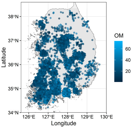
Figure 1.
Spatial distribution of the field data (n = 9584). Points are field-wide averages of organic matter (OM; g kg−1) for the period of 2020 to early 2023.
Table 2.
Descriptive statistics of numeric data (n = 9584).
We obtained the digital elevation model (DEM) data (90 m resolution) (Table 2), which represented a continuous topographic elevation surface, from the National Spatial Data Infrastructure (NSDI) portal [32]. We used the DEM data to derive slope, aspect, roughness, topographic position index, terrain ruggedness index, and flow direction. Hill shade was computed from slope and aspect [35], assuming sun elevation and direction (azimuth) angles of 45° and 0°, respectively. Lastly, we estimated the upslope contributing area and topographic wetness index according to Quinn et al. [36]. We used a global estimate of annual net primary production in TIFF format from 2019 to 2021 to represent vegetation from the Moderate Resolution Imaging Spectroradiometer (MODIS) aboard NASA’s Terra and Aqua satellites [34]. The spatial resolution of the data is 0.1° (approximately 11 km). To represent the current climate, we used mean annual air temperature, maximum/minimum air temperature, mean annual precipitation, solar irradiation, relative humidity, and wind speed data based on the Modified Korean-Parameter-elevation Regressions on Independent Slopes Model (MK-PRISM, version 1.2). All data were available from 2000 to 2019, except for solar irradiation (2014–2019) [33]. The MK-PRISM data were in netCDF format. All climatic variables were averaged annually and then over the entire period, whereas the sum of precipitation values was calculated and averaged over the same period.
According to the land cover data from EGIS [37], agricultural land subclasses include the following: (1) fields (including rearranged fields), (2) rice paddies, (3) facility cultivation, (4) orchards, and (5) pastures and nurseries. Based on the survey of arable land in 2021 [38], the total field area was 766,000 ha. We first compiled valid soil chemical data and the coordinates of the fields (n = 310,716). We then extracted the values of the climate, terrain, and soil map variables with the coordinates of the samples. We removed outliers from the complete dataset based on Cook’s distance (n = 9584) and scaled the data for modeling. All data were compiled and processed in R (version 4.3.1) [39].
2.2. Explainable Tree-Based Models
Several reviews provide an overview of ML models [40,41]. One of the benefits of ML is the ability to learn vast amounts of data by exploiting the variation in resources from observation and related environmental covariates [42]. Tree-based modeling is the most used learning technology in soil mapping. We chose decision tree (DT), random forest (RF), and gradient boosting (GB) due to their ease of interpretation and proven success in handling structured datasets [43]. The DT algorithm is a recursive partitioning method that iteratively generates child nodes, further divided into pairs of nodes. DT serves as an interpretable ML model, as the decision path from the root to the leaf or terminal nodes keeps track of the features used for predictions. However, DT learning is difficult to comprehend and suffers from overfitting when the models become more complex (i.e., with a larger maximum depth).
Ensemble methods, such as RF and GB, are used instead to address this issue. By incorporating multiple decision trees, these approaches produce robust and accurate models. Leveraging the diversity of individual trees, they mitigate overfitting while enhancing overall performance. RF uses feature randomization to create each tree. At each split, a random subset of features is considered to determine the best splitting point for the node. This randomness increases the diversity among trees and enhances the generalization capability of the ensemble model. GB is an alternative ensemble learning technique in which an additive model is constructed by sequentially combining predictions from multiple decision trees, thus creating a robust predictive model. RF primarily aims to reduce variance through subset (i.e., bagging) and feature randomization. In contrast, GB focuses on diminishing bias and enhancing predictive accuracy through iterative optimization processes. Among the models, the DT algorithm is relatively simple, and its interpretability is high. The RF and GB models are composed of many trees that have been combined, which, therefore, must be supplemented with interpretable methods for understanding model behavior.
2.2.1. Model Evaluation
We integrated the Shapley additive explanation (SHAP) method, developed by Lundberg and Lee [44], with the optimized ML to interpret the prediction criteria of the models and the level of contribution of the individual features that strongly correlate in organic matter prediction. Feature importance provides a crucial reference for feature selection [45]. A higher feature importance value, compared with another, implies the greater importance of the feature for generating a prediction. Shapley values quantify the contribution of each explanatory variable in each instance. The term “additive” signifies that the corresponding Shapley value for each explanatory variable of an instance can be additively combined [46]. This approach provides quantitative information to explain how individual explanatory variables either positively or negatively impact the target variable of interest in the model. The following formula represents the Shapley value, ϕi(v):
where v(S) represents the output of the ML model being explained with a set S of features, and N refers to the entire set of available features. The Shapley value or contribution of a specific feature i () is calculated as the average contribution across all possible permutations of the feature set [47], akin to determining the marginal contribution (. This method evaluates the unique impact of feature i by assessing how the inclusion or exclusion of this feature alters the model’s output, mirroring the process of assessing a feature’s extra value in the model. Additionally, it applies a weighting factor () to account for every potential combination of features, ensuring that the influence of each feature is measured fairly and equitably. Lastly, summing over all coalitions and normalizing with denominator aggregates the contributions of each feature to recognize the significance of individual features in proportion to their effect on the model’s performance.
The Shapley-based feature importance method, however, does not provide insights into two crucial aspects: (1) how changes in these important features affect predictions and (2) whether a specific threshold for these key features can enhance the accuracy of predicting the target variable. To address these concerns, we employed partial dependence (PD) plotting, which enabled us to analyze how specific input features contribute to variations in the expected response of the target variable. One-dimensional PD plots illustrate how changes in the chosen independent variables impact the expected value of their dependent variable while other independent variables remain constant. Furthermore, two-dimensional PD plots are used to assess predicted values for their dependent variable as both independent variables simultaneously vary.
PD plots are a tool for comprehending the impacts of features in any ML model [48], such as (x). The explanatory variables x = (, ) can be divided into two subsets to emphasize the concept and effectively convey this relationship and visualization: and . represents the “chosen” independent variable, and comprises the set of other independent variables. The function that represents PD is defined as follows:
represents the partial dependence of a subset of features on the model’s predictions, illustrating how the average prediction changes when the values of are altered while all other variables () remain constant. The term signifies the calculation of an average, where the model’s predictions for each instance (from 1 to n, with n being the total number of instances in the dataset) are then divided by n. The prediction function, , calculates the prediction for each combination , and the other features , enabling the assessment of how changes in , alone influence the model’s predictions.
2.2.2. Assessment Statistics
To train the model, we performed five-times repeated fivefold cross-validation. Grid searching was employed for exhaustive searching to systematically tune the hyperparameters in ML from a predefined set of values to enhance performance and mitigate the risk of overfitting (Table 3).
Table 3.
Optimal hyperparameters of three tree-based models.
To assess the performance of the models, we computed the root mean squared error (RMSE) to quantify the inaccuracy of the estimates, the mean absolute error (MAE) to quantify the errors between modeled and observed values, and the coefficient of determination (R2). The RMSE accounts for both the bias and the imprecision of the analysis. We report the mean and standard deviation of the assessment statistics from the cross-validations.
3. Results
3.1. Comparison of Selected Tree-Based Models
Among the models, GB exhibited the best performance, as indicated by the highest R2 of 0.59 (Figure 2). Following closely, RF demonstrated comparable predictive ability with an R2 of 0.57. Lastly, the DT model displayed the weakest performance, with an R2 of 0.45. Furthermore, the RF and GB models exhibited higher prediction accuracy with fewer errors. Moreover, these two models showed a more concentrated distribution of estimates around the observations, suggesting increased consistency and reliability in their predictions compared with those of the DT model (Figure 2).
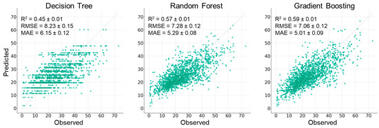
Figure 2.
Scatter plots of predicted-versus-observed organic matter stocks in soil by using tree-based model. Points are field-wide averages for the last three years (2020–early 2023). Dashed line is 1:1.
The optimal values for the hyperparameters of each model used in the study are summarized in Table 3. For the DT model, a maximum depth of six was selected to prevent overfitting caused by the excessive expansion of the tree structure. The minimum number of samples per node was set to 12. In the RF model, a maximum depth of 12 and a minimum number of eight samples per leaf were chosen. In the GB model, a maximum depth of eight and a minimum number of 18 samples per leaf were chosen. Additionally, an internal node requires at least eight samples for splitting to manage complexity and minimize overfitting concerns. Our RF and GB models comprised 100 trees to ensure accurate results. However, adding more trees beyond this point yielded no further improvements.
3.2. Feature Overall Importance Analysis
The global feature explanation obtained from the SHAP method for the three tree-based models is shown in Figure 3 and Figure 4. We represent the average impact of each variable on soil organic matter based on the global feature importance, which is the mean absolute representative SHAP value for that feature over all the given samples (Figure 3). Figure 4 illustrates the impact of the features on the model’s predictions. Higher SHAP values for precipitation, indicated in red, signify a large and positive average impact on predictions, suggesting a higher likelihood of increasing the prediction accuracy due to the high mean absolute SHAP values.
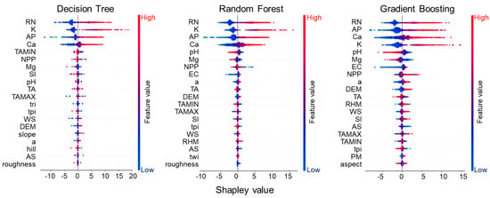
Figure 3.
Global feature explanation through the Shapley additive explanation for three tree-based models. The range of Shapley values was computed for each explanatory variable to determine its impact on soil organic matter content. For abbreviations, refer to Table 1.
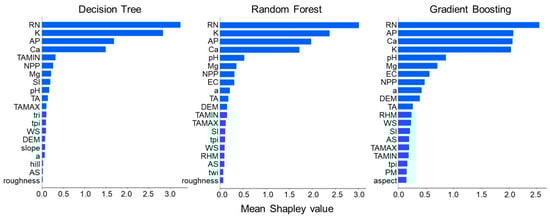
Figure 4.
Shapley-based feature importance of environmental variables for global explanations of soil organic matter content, expressed as mean Shapley values. For abbreviations, refer to Table 1.
The features are ordered from top to bottom by their predictive importance. In this case, we found that all models consistently identified the mean annual precipitation as the primary predictor. This was closely trailed by exchangeable K content in the DT and RF models (Figure 4). Similarly, the GB model acknowledged exchangeable K as one of the top five predictors; however, it attributed relatively less importance to it (Figure 4).
3.3. Feature Partial Dependence Analysis
Subsequently, we undertook a more in-depth investigation into the impacts of precipitation and exchangeable K on soil organic matter content. This choice was driven by the results of the DT and RF analyses, which highlighted these variables as being within the top two regarding Shapley-based feature importance (Figure 3 and Figure 4). In Figure 5, we present PD plots illustrating how the three models portrayed the connections between precipitation and organic matter content; all models consistently showed a positive correlation between them. Nonetheless, we identified disparities in the strength and form of the relationships across the models. Specifically, the DT model exhibited a distinct, step-like association centered around a precipitation value of 1400 mm (Figure 5). However, both RF and GB models suggested a positive yet nonlinear relationship.
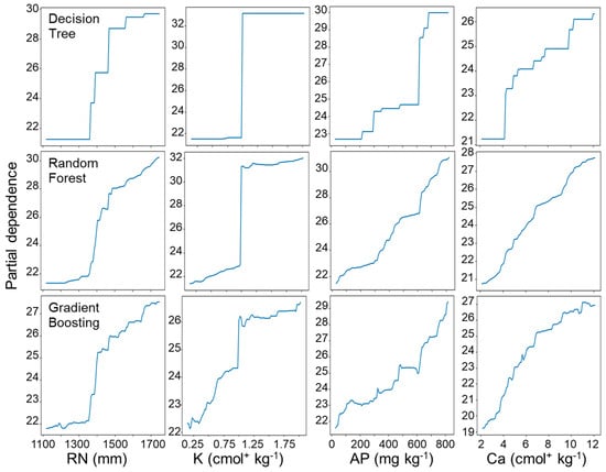
Figure 5.
Partial dependence plots of soil organic matter content with precipitation (RN), exchangeable potassium (K), available phosphate (AP), and exchangeable calcium (Ca) (global explanations).
When scrutinizing the association between soil organic matter content and other variables, all three models concurred on the positive nature of these relationships for precipitation, exchangeable K, and available P. Notably, only the DT model revealed a conspicuous stepwise linkage, discernible at the values of precipitation (1400 mm), K (1 cmol+ kg−1), and available P (600 mg kg−1).
Two-dimensional PD plots were employed to visually determine the interaction effects between precipitation and exchangeable K (Figure 6). All models indicated that organic matter is contingent upon both precipitation and K. The observed patterns across all models displayed distinct divisions in the patterns along the K contents around the value of 1 cmol+ kg−1 and along the amount of precipitation of approximately 1400 mm. This observation strongly suggests the presence of an interaction effect between these variables. The presentation of PD plots focusing on precipitation while conditioning on varying K thresholds effectively demonstrates this interaction effect (Figure 6). Specifically, as precipitation increased within the 1400–1700 mm range, the RF model showed a more gradual rise in soil organic matter content from 30.53 g kg−1 to 33.66 g kg−1 and 36.79 g kg−1, smoothing out the potential anomalies through averaging multiple outputs, while the GB model displayed fluctuations, with predicted values falling from 7.48 g kg−1 to 4.82 g kg−1 before rising again to 7.48 g kg−1, due to its sequential approach that may capture complex patterns as well as anomalies.
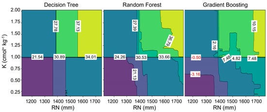
Figure 6.
Partial dependence of soil organic matter between precipitation (RN) and exchangeable potassium (K). The numbers on the plot are the predicted value of soil organic matter in g kg−1.
In contrast, for DT and RF, the most important variables are precipitation and K, while for GB, the most crucial variables are precipitation and P, with K ranking fourth in importance, suggesting why there were fluctuations. The GB model recognized exchangeable K as one of the top five predictors but assigned it relatively lower importance (Figure 4), indicating a different predictive behavior that might lead to the observed fluctuations. In contrast, the DT showed a different type of fluctuation, where the predicted values shifted from 30.89 g kg−1 to 37.13 g kg−1 and then settled at 34.01 g kg−1, potentially reflecting overfitting to the training data, resulting in abrupt threshold effects. A discernible pattern emerges from these plots, showing that the association with precipitation exhibits heightened strength when the level of exchangeable K surpasses 1 cmol+ kg−1.
4. Discussion
Tree-based modeling can lead to the reliable prediction of organic matter content in soil (Figure 2). Based on the model performance analysis results, we found that GB explained 59% of the nationwide variation in soil organic matter and yielded the highest accuracy among the models evaluated, followed by RF and then DT. The precipitation variable consistently emerged as the most influential predictor in all these models under Korean conditions. Therefore, the results suggest that the promotion of supplemental irrigation is necessary for sustainable crop production due to changes in precipitation [49,50]. Subsequently, we found that soil organic matter content under field crops also depended on soil macronutrients, such as K, P, and Ca levels. Since the soil supply of these nutrients is often supplemented by fertilizer, this suggests the importance of efficient soil fertility management under variable climates. In addition, analyzing the bee swarm summary plots provided a more comprehensive understanding of how other variables influenced the prediction (Figure 3 and Figure 4). Here, GB uniquely identified precipitation and available P as the most influential variables, unlike DT and RF, which prioritized precipitation and K. Such differences in captured feature importance in complex data might account for improved predictive accuracy. All models revealed positive relationships between macronutrients and soil organic matter (Figure 5), but the intensity and shape of these relationships varied among the models. For example, the two-dimensional PD plots illustrated the divergent interaction effects of precipitation and exchangeable K (Figure 6). The findings suggested that the relationship with organic matter is more robust when exchangeable K exceeds 1 cmol+ kg−1 and annual precipitation surpasses 1400 mm. Thus, organic matter content is contingent upon both precipitation and K on a large scale, suggesting specific field conditions where practices effectively increase soil organic matter [51]. This assessment comprehensively explains the varying importance levels attributed to main predictors using distinct modeling approaches. However, the impact of these features on the model is still not fully understood [52].
Only the DT model revealed a conspicuous stepwise linkage, discernible at specific values of precipitation (1400 mm), available P (600 mg kg−1), and K (1 cmol+ kg−1) (Figure 5). The DT model tended to create distinct, threshold-based splits in the data. In contrast, the RF and GB models captured smoother and more nonlinear relationships that offer a comprehensive understanding of how variables incrementally affect soil organic matter in a more detailed and integrated manner. This PD analysis underscores the nuances in how different models represent the intricate interplay between soil variables and organic matter. This insight provides valuable clarity regarding these two variables’ complex interplay and collective impact on soil organic matter. Up to this point, our focus was on elucidating the overarching behavior of global models, aiming to comprehend the insights derived from the data. However, this approach falls short in explaining the nuances of local model behavior, a critical aspect in discerning the factors deemed important by the models when predicting values for specific instances. We also employed the SHAP method to assess the importance of variables at a specific local site. The results indicated that pH was more important than precipitation, identified as the most influential factor in controlling global model behavior. Therefore, future research is needed to gain a more general understanding of local factors and site-specific targeting for more efficient organic matter management.
Tree-based modeling, using Shapley values, can lead to the identification of vital environmental factors that affect organic matter content nationwide. This knowledge is essential for managing the soil’s health and the sustainability of cropping systems and for fine-tuning fertilizer and water use management. Moreover, when addressing agricultural challenges, especially with adopting alternative production systems [53,54], the results can support the selection of a farm location to improve not only soil organic matter and fertility conditions but also the marketability and profitability of crop harvests. For example, in Kenya, agricultural practices include the use of fertilizers, pesticides, and irrigation to enhance soil organic matter, potentially producing premium-market-priced organic products [55]. When premium prices are available for organic produce, the organic system yields significantly higher net returns than conventionally managed systems, achieving a gross margin that is 1.3 to 4.1 times higher. Additionally, intercropping various crops enhanced overall productivity and profitability [55]. Thus, these results provide insights into the economic implications of choosing an alternative farming system based on soil organic matter levels and related conditions. In enhancing soil organic matter content, several viable management approaches may offer additional means to boosting agricultural productivity, including soil amendment; yet, the economic evaluation of each of these methods has been limited, and a gap exists in terms of the comprehensive evaluation of the socioeconomic impacts, necessitating further research in this area. Petersen and Hoyle [56] modeled the benefits of soil organic carbon, mainly focusing on the increased availability of nitrogen and increased plant-available water-holding capacity (PAWC). The value of soil organic carbon is estimated to be between AUD 7.1 and 8.7 Mg−1 ha−1 annually. This valuation includes approximately 75% for carbon sequestration and smaller proportions for productivity improvements. The enhancements in PAWC (~5%) and nitrogen replacement value (~20%) contribute to higher agricultural productivity. An increased PAWC allows for increased water retention in the soil, and increased nitrogen availability supports healthier plant growth. Both soil quality and profit result in higher-quality land having a higher market value, providing an additional incentive to adopt a soil-conserving crop production system.
Mikhailova et al. [57] evaluated the monetary value of soil organic carbon stocks in the U.S., considering various factors such as soil order, depth, and geographic region. They estimated the total value of soil organic carbon storage to range from USD 4.64 trillion to USD 23.1 trillion. This valuation highlights the critical role of its management in delivering environmental and economic benefits. Similarly, Dube et al. [58] offered a detailed financial analysis of ecosystem services from healthy soils in Vermont, highlighting benefits such as increased carbon storage (USD 19 acre−1 year−1 in climate mitigation), reduced phosphorus losses (USD 8 acre−1 year−1 in water quality), erosion control (USD 2 acre−1 year−1 in waterway damage reduction), and enhanced water retention (USD 2 acre−1 year−1 in flood damage reduction), cumulatively valued at over USD 25 million annually. This emphasizes the economic importance of soil health investment and preservation. Hacisalihoglu et al. [59] used the “market value of soil” method to calculate the cost of soil erosion, considering nutrient loss and fertilizer market prices. They estimated an average economic loss of USD 59.54 per hectare per year in pasture lands and USD 102.36 in agricultural lands in Turkey due to soil erosion. This erosion, which tends to remove the nutrient- and organic-matter-rich topsoil, diminishes soil fertility, provides nutrients, sustains structure and moisture, and affects economic values by depleting a crucial soil component. Additionally, Kane et al. [60] found that counties with higher soil organic matter levels had increased yields, lower yield losses, and lower crop insurance payout rates. A 1% increase in soil organic matter corresponded to a yield boost of 2.2 ± 0.33 Mg ha−1 and a notable reduction of 36 ± 4.76% in the average proportion of liabilities paid. Sparling et al. [61] quantified the monetary value of soil organic matter in enhancing crop production in New Zealand soils. This value was determined by estimating the worth of dairy milk solids, derived from a computer simulation modeling the yield of dry pasture matter and the accumulation of organic matter. The findings revealed that soils with lower organic matter levels yielded between 8.5 and 47.7 kg fewer milk solids per hectare annually, translating to a financial impact of NZD 27 to NZD 150 per hectare. Over recovery periods of 36, 90, and 125 years, the cumulative loss per hectare at Pukekohe, due to reduced productivity, was estimated to be NZD 1239 with a 3.5% discount factor and NZD 772 with a 10% discount.
Finally, Fan et al. [62] showed that field practices with varying organic matter inputs could affect the total ecosystem service valuation in organic cereal crop production systems. This impact likely stems from altered soil properties due to long-term diverse field management. The authors estimated the economic value of ES in these systems under different management strategies, finding that the economic values ranged from USD 1492 to USD 1969 per hectare per year. Reyes and Elias [63] demonstrated that drought and excess precipitation were the primary causes of crop losses in the U.S. from 2001 to 2016, leading to over USD 440 billion in economic damage. These studies emphasize the importance of understanding and predicting environmental factors in agriculture. Therefore, tree-based modeling for predicting organic matter in soil and identifying key factors can help improve soil health and contribute to more sustainable and profitable agricultural practices.
5. Conclusions
We introduced the SHAP method to address the lack of interpretability of ML modeling to gain more insight into large-scale agricultural management. Specifically, we selected three tree-based models (decision tree, random forest, and gradient boosting) and focused on the global factors contributing to the soil organic matter content across the fields. We found that tree-based explainable ML enables the reliable prediction of the organic matter content in soil and identifies vital environmental factors that are relevant to organic matter management. Soil organic matter, as an example, can provide multiple benefits as a valuable resource but represents challenges commonly faced in agriculture. This new knowledge is essential but still limited in terms of managing soil health and the sustainability of cropping systems and fine-tuning fertilizer and water use management. Therefore, our approaches can be applied to the sustainable management of other agricultural resources at a large scale. We further examined the potential interactions between selected variables within the top four as determined by the Shapley-based feature importance. Based on our results, we need to further consider incorporating deep learning into our analytical framework to provide considerable benefit. Deep learning has demonstrated remarkable capabilities in handling complex data patterns and may provide enhanced insights when applied to agricultural science. For future studies, our prior emphasis on overall feature importance analysis should complement the uncertain contribution of local factors. Whereas overall feature importance analysis provides valuable insights at the global level, there is the need for local analysis, which allows for a more granular understanding of how specific features impact the system under investigation. This perspective can lead to more precise and actionable recommendations for resource management. Lastly, employing feature elimination represents a meaningful avenue for analysis. This approach can aid with dimensionality reduction and identifying critical features, potentially simplifying the model while preserving its predictive power. Such streamlining can enhance model interpretability and efficiency, which are paramount in agricultural science.
Author Contributions
J.L. formulated the research. W.L. performed data modeling and analysis. W.L. and J.L. wrote the manuscript. All authors have read and agreed to the published version of the manuscript.
Funding
This study was funded by the National Research Foundation of Korea (NRF), NRF-2022R1F1A1073973.
Institutional Review Board Statement
Not applicable.
Informed Consent Statement
Not applicable.
Data Availability Statement
The datasets generated during and analyzed during the current study are available from the corresponding author upon reasonable request.
Conflicts of Interest
The authors declare no conflicts of interest. The funders had no role in the design of the study; in the collection, analyses, or interpretation of data; in the writing of the manuscript; or in the decision to publish the results.
References
- Bodria, F.; Giannotti, F.; Guidotti, R.; Naretto, F.; Pedreschi, D.; Rinzivillo, S. Benchmarking and survey of explanation methods for black box models. Data Min. Knowl. Discov. 2021, 37, 1719–1778. [Google Scholar] [CrossRef]
- Ryo, M. Explainable artificial intelligence and interpretable machine learning for agricultural data analysis. Artif. Intell. Agric. 2022, 6, 257–265. [Google Scholar] [CrossRef]
- Miller, T. Explanation in Artificial Intelligence: Insights from the Social Sciences. Artif. Intell. 2017, 267, 1–38. [Google Scholar] [CrossRef]
- Belle, V.; Papantonis, I. Principles and practice of explainable machine learning. Front. Big Data 2021, 4, 688969. [Google Scholar] [CrossRef]
- Saeed, W.; Omlin, C. Explainable AI (XAI): A systematic meta-survey of current challenges and future opportunities. Knowl.-Based Syst. 2023, 263, 110273. [Google Scholar] [CrossRef]
- Wang, M.; Fu, W.J.; He, X.N.; Hao, S.J.; Wu, X.D. A survey on large-scale machine learning. IEEE Trans. Knowl. Data Eng. 2022, 34, 2574–2594. [Google Scholar] [CrossRef]
- Visser, O.; Sippel, S.R.; Thiemann, L. Imprecision farming? Examining the (in)accuracy and risks of digital agriculture. J. Rural Stud. 2021, 86, 623–632. [Google Scholar] [CrossRef]
- Dundon, S.J. Agricultural ethics and multifunctionality are unavoidable. Plant Physiol. 2003, 133, 427–437. [Google Scholar] [CrossRef] [PubMed]
- Rudin, C. Stop explaining black box machine learning models for high stakes decisions and use interpretable models instead. Nat. Mach. Intell. 2019, 1, 206–215. [Google Scholar] [CrossRef]
- Finger, R. Digital innovations for sustainable and resilient agricultural systems. Eur. Rev. Agric. Econ. 2023, 50, 1277–1309. [Google Scholar] [CrossRef]
- Hoang, N.T.; Taherzadeh, O.; Ohashi, H.; Yonekura, Y.; Nishijima, S.; Yamabe, M.; Matsui, T.; Matsuda, H.; Moran, D.; Kanemoto, K. Mapping potential conflicts between global agriculture and terrestrial conservation. Proc. Natl. Acad. Sci. USA 2023, 120, e2208376120. [Google Scholar] [CrossRef]
- Chouldechova, A. Fair prediction with disparate impact: A study of bias in recidivism prediction instruments. Big Data 2016, 5, 153–163. [Google Scholar] [CrossRef] [PubMed]
- Schuett, J. Risk management in the Artificial Intelligence Act. Eur. J. Risk Regul. 2023, 1–19. [Google Scholar] [CrossRef]
- Thomson Reuters. LAWnB IP Exclusive Report: 2023 Domestic and International AI Regulatory and Policy Trends; Thomson Reuters Korea: Seoul, Korea, 2023; pp. 5–8. [Google Scholar]
- Breiman, L. Statistical modeling: The two cultures. Stat. Sci. 2001, 16, 133. [Google Scholar] [CrossRef]
- Guidotti, R.; Monreale, A.; Turini, F.; Pedreschi, D.; Giannotti, F. A survey of methods for explaining black box models. ACM Comput. Surv. 2018, 51, 1–42. [Google Scholar] [CrossRef]
- Adadi, A.; Berrada, M. Peeking inside the black-box: A survey on explainable artificial intelligence (XAI). IEEE Access 2018, 6, 52138–52160. [Google Scholar] [CrossRef]
- Barredo Arrieta, A.; Díaz-Rodríguez, N.; Del Ser, J.; Bennetot, A.; Tabik, S.; Barbado, A.; Garcia, S.; Gil-Lopez, S.; Molina, D.; Benjamins, R.; et al. Explainable Artificial Intelligence (XAI): Concepts, taxonomies, opportunities and challenges toward responsible AI. Inf. Fusion 2020, 58, 82–115. [Google Scholar] [CrossRef]
- Theissler, A.; Spinnato, F.; Schlegel, U.; Guidotti, R. Explainable AI for time series classification: A review, taxonomy and research directions. IEEE Access 2022, 10, 100700–100724. [Google Scholar] [CrossRef]
- Yuan, H.; Yu, H.; Gui, S.; Ji, S. Explainability in graph neural networks: A taxonomic survey. IEEE Trans. Pattern Anal. Mach. Intell. 2020, 45, 5782–5799. [Google Scholar] [CrossRef]
- Pichler, M.; Hartig, F. Machine learning and deep learning—A review for ecologists. Methods Ecol. Evol. 2023, 14, 994–1016. [Google Scholar] [CrossRef]
- Rudin, C.; Chen, C.; Chen, Z.; Huang, H.; Semenova, L.; Zhong, C. Interpretable machine learning: Fundamental principles and 10 grand challenges. Stat. Surv. 2022, 16, 85. [Google Scholar] [CrossRef]
- Antle, J.M.; Basso, B.; Conant, R.T.; Godfray, H.C.J.; Jones, J.W.; Herrero, M.; Howitt, R.E.; Keating, B.A.; Munoz-Carpena, R.; Rosenzweig, C.; et al. Towards a new generation of agricultural system data, models and knowledge products: Design and improvement. Agric. Syst. 2017, 155, 255–268. [Google Scholar] [CrossRef] [PubMed]
- Smith, P.; Davies, C.A.; Ogle, S.; Zanchi, G.; Bellarby, J.; Bird, N.; Boddey, R.M.; McNamara, N.P.; Powlson, D.; Cowie, A.; et al. Towards an integrated global framework to assess the impacts of land use and management change on soil carbon: Current capability and future vision. Glob. Chang. Biol. 2012, 18, 2089–2101. [Google Scholar] [CrossRef]
- Hu, T.; Zhang, X.; Bohrer, G.; Liu, Y.; Zhou, Y.; Martin, J.; Li, Y.; Zhao, K. Crop yield prediction via explainable AI and interpretable machine learning: Dangers of black box models for evaluating climate change impacts on crop yield. Agric. For. Meteorol. 2023, 336, 109458. [Google Scholar] [CrossRef]
- Paustian, K.; Lehmann, J.; Ogle, S.; Reay, D.; Robertson, G.P.; Smith, P. Climate-smart soils. Nature 2016, 532, 49–57. [Google Scholar] [CrossRef]
- Lal, R. Challenges and opportunities in soil organic matter research. Eur. J. Soil Sci. 2009, 60, 158–169. [Google Scholar] [CrossRef]
- Conway, G.R. The properties of agroecosystems. Agric. Syst. 1987, 24, 95–117. [Google Scholar] [CrossRef]
- Spencer, J.E.; Stewart, N.R. The nature of agricultural systems. Ann. Assoc. Am. Geogr. 1973, 63, 529–544. [Google Scholar] [CrossRef]
- NAS. Chemical Data for Soil Test. National Institute of Agricultural Sciences, Rural Development Administration 2023. Available online: www.data.go.kr/data/15073569/openapi.do (accessed on 30 January 2023).
- RDA. Precision Soil Maps. Rural Development Administration 2023. Available online: https://soil.rda.go.kr (accessed on 19 January 2023).
- NSDI. Degital Elevation Model. National Spatial Data Infrastructure 2020. Available online: https://data.nsdi.go.kr/dataset/20001 (accessed on 11 August 2020).
- KMA. Climate Change Scenarios. 2023. Available online: https://www.climate.go.kr/home/CCS/contents_2021/35_download.php (accessed on 20 December 2023).
- NEO. Net Primary Productivity (1 year—TERRA/MODIS). NASA Earth Observations 2023. Available online: https://neo.gsfc.nasa.gov (accessed on 20 February 2023).
- Horn, B.K.P. Hill shading and the reflectance map. Proc. IEEE 1981, 69, 14–47. [Google Scholar] [CrossRef]
- Quinn, P.F.; Beven, K.J.; Lamb, R. The in(a/tan/β) index: How to calculate it and how to use it within the topmodel framework. Hydrol. Process. 1995, 9, 161–182. [Google Scholar] [CrossRef]
- EGIS. Land Cover Maps. Environmental Geographic Information Service 2023. Available online: https://egis.me.go.kr/intro/land.do (accessed on 13 January 2023).
- Statistics Korea. Arable land in Korea. 2021. Available online: https://kosis.kr/statHtml/statHtml.do?orgId=101&tblId=DT_1EB001&conn_path=I2 (accessed on 6 October 2022).
- R Core Team. R: A Language and Environment for Statistical Computing; R Foundation for Statistical Computing: Vienna, Austria, 2023. [Google Scholar]
- Heung, B.; Ho, H.C.; Zhang, J.; Knudby, A.; Bulmer, C.E.; Schmidt, M.G. An overview and comparison of machine-learning techniques for classification purposes in digital soil mapping. Geoderma 2016, 265, 62–77. [Google Scholar] [CrossRef]
- Alzubaidi, L.; Zhang, J.; Humaidi, A.J.; Al-Dujaili, A.; Duan, Y.; Al-Shamma, O.; Santamaría, J.; Fadhel, M.A.; Al-Amidie, M.; Farhan, L. Review of deep learning: Concepts, CNN architectures, challenges, applications, future directions. J. Big Data 2021, 8, 53. [Google Scholar] [CrossRef] [PubMed]
- Lagacherie, P. Digital Soil Mapping: A State of the Art. In Digital Soil Mapping with Limited Data; Hartemink, A.E., McBratney, A., Mendonça-Santos, M.d.L., Eds.; Springer: Dordrecht, The Netherlands, 2008; pp. 3–14. [Google Scholar]
- Hastie, T.; Tibshirani, R.; Friedman, J. Unsupervised Learning. In The Elements of Statistical Learning: Data Mining, Inference, and Prediction; Hastie, T., Tibshirani, R., Friedman, J., Eds.; Springer: New York, NY, USA, 2009; pp. 485–585. [Google Scholar]
- Lundberg, S.M.; Lee, S.-I. A Unified Approach to Interpreting Model Predictions. In Proceedings of the 31st International Conference on Neural Information Processing Systems, Long Beach, CA, USA, 4–9 December 2017; pp. 4768–4777. [Google Scholar]
- Zhang, W.; Wu, C.; Zhong, H.; Li, Y.; Wang, L. Prediction of undrained shear strength using extreme gradient boosting and random forest based on Bayesian optimization. Geosci. Front. 2021, 12, 469–477. [Google Scholar] [CrossRef]
- Liu, J.; Li, C.; Ouyang, P.; Liu, J.; Wu, C. Interpreting the prediction results of the tree-based gradient boosting models for financial distress prediction with an explainable machine learning approach. J. Forecast. 2023, 42, 1112–1137. [Google Scholar] [CrossRef]
- Rodríguez-Pérez, R.; Bajorath, J. Interpretation of machine learning models using shapley values: Application to compound potency and multi-target activity predictions. J. Comput.-Aided Mol. Des. 2020, 34, 1013–1026. [Google Scholar] [CrossRef] [PubMed]
- Friedman, J.H. Greedy function approximation: A gradient boosting machine. Ann. Stat. 2001, 29, 1189–1232. [Google Scholar] [CrossRef]
- Lundy, M.E.; Pittelkow, C.M.; Linquist, B.A.; Liang, X.Q.; van Groenigen, K.J.; Lee, J.; Six, J.; Venterea, R.T.; van Kessel, C. Nitrogen fertilization reduces yield declines following no-till adoption. Field Crop. Res. 2015, 183, 204–210. [Google Scholar] [CrossRef]
- Pittelkow, C.M.; Linquist, B.A.; Lundy, M.E.; Liang, X.Q.; van Groenigen, K.J.; Lee, J.; van Gestel, N.; Six, J.; Venterea, R.T.; van Kessel, C. When does no-till yield more? A global meta-analysis. Field Crop. Res. 2015, 183, 156–168. [Google Scholar] [CrossRef]
- Machmuller, M.B.; Kramer, M.G.; Cyle, T.K.; Hill, N.; Hancock, D.; Thompson, A. Emerging land use practices rapidly increase soil organic matter. Nat. Commun. 2015, 6, 6995. [Google Scholar] [CrossRef]
- Czerwinska, U. Interpretability of Machine Learning Models. In Applied Data Science in Tourism: Interdisciplinary Approaches, Methodologies, and Applications; Egger, R., Ed.; Springer International Publishing: Cham, Switzerland, 2022; pp. 275–303. [Google Scholar]
- Pittelkow, C.M.; Liang, X.Q.; Linquist, B.A.; van Groenigen, K.J.; Lee, J.; Lundy, M.E.; van Gesell, N.; Six, J.; Venterea, R.T.; van Kessel, C. Productivity limits and potentials of the principles of conservation agriculture. Nature 2015, 517, 365-U482. [Google Scholar] [CrossRef]
- Petersen, B.; Snapp, S. What is sustainable intensification? Views from experts. Land Use Policy 2015, 46, 1–10. [Google Scholar] [CrossRef]
- Adamtey, N.; Musyoka, M.W.; Zundel, C.; Cobo, J.G.; Karanja, E.; Fiaboe, K.K.M.; Muriuki, A.; Mucheru-Muna, M.; Vanlauwe, B.; Berset, E.; et al. Productivity, profitability and partial nutrient balance in maize-based conventional and organic farming systems in Kenya. Agric. Ecosyst. Environ. 2016, 235, 61–79. [Google Scholar] [CrossRef]
- Petersen, E.H.; Hoyle, F.C. Estimating the economic value of soil organic carbon for grains cropping systems in Western Australia. Soil Res. 2016, 54, 383–396. [Google Scholar] [CrossRef]
- Mikhailova, E.A.; Groshans, G.R.; Post, C.J.; Schlautman, M.A.; Post, G.C. Valuation of soil organic carbon stocks in the contiguous United States based on the avoided social cost of carbon emissions. Resources 2019, 8, 153. [Google Scholar] [CrossRef]
- Dube, B.; White, A.; Ricketts, T.; Darby, H. Valuation of Soil Health Ecosystem Services; The University of Vermont: Burlington, VT, USA, 2022. [Google Scholar]
- Hacisalihoglu, S.; Toksoy, D.; Kalca, A. Economic valuation of soil erosion in a semi and area in Turkey. Afr. J. Agric. Res. 2010, 5, 1–6. [Google Scholar] [CrossRef]
- Kane, D.A.; Bradford, M.A.; Fuller, E.; Oldfield, E.E.; Wood, S.A. Soil organic matter protects US maize yields and lowers crop insurance payouts under drought. Environ. Res. Lett. 2021, 16, 044018. [Google Scholar] [CrossRef]
- Sparling, G.P.; Wheeler, D.; Vesely, E.T.; Schipper, L.A. What is soil organic matter worth? J. Environ. Qual. 2006, 35, 548–557. [Google Scholar] [CrossRef]
- Fan, F.; Henriksen, C.B.; Porter, J. Valuation of ecosystem services in organic cereal crop production systems with different management practices in relation to organic matter input. Ecosyst. Serv. 2016, 22, 117–127. [Google Scholar] [CrossRef]
- Reyes, J.J.; Elias, E. Spatio-temporal variation of crop loss in the United States from 2001 to 2016. Environ. Res. Lett. 2019, 14, 074017. [Google Scholar] [CrossRef]


Disclaimer/Publisher’s Note: The statements, opinions and data contained in all publications are solely those of the individual author(s) and contributor(s) and not of MDPI and/or the editor(s). MDPI and/or the editor(s) disclaim responsibility for any injury to people or property resulting from any ideas, methods, instructions or products referred to in the content. |
© 2024 by the authors. Licensee MDPI, Basel, Switzerland. This article is an open access article distributed under the terms and conditions of the Creative Commons Attribution (CC BY) license (https://creativecommons.org/licenses/by/4.0/).