Abstract
Aiming at the shortcomings of the existing machine vision pose measurement technology, a pose measurement method based on monocular vision and a cooperative target is proposed. A planar target designed with circles and rings as the main body is dedicated to object pose measurement, and a feature point coordinate extraction and sorting algorithm is designed for this target to effectively extract image features on the target. The RANSAC algorithm and topology-based fitting for the intersection method are used to optimise data processing, further improving the accuracy of feature point coordinate extraction and ultimately achieving high-precision measurement of object poses. The experimental results show that the measurement accuracy of the roll angle perpendicular to the optical axis can reach 0.02°, and the repeatability can reach 0.0004° after removing the systematic error; the measurement accuracy of the pitch angle can reach 0.03°, and the repeatability can go to 0.002° after removing the systematic error. The measurement range of the pitch angle is [−30°, +30°]; the measurement range of the roll angle is [−179°, +179°]. The experimental results show that the system has high measurement accuracy and meets the requirements of high-precision measurement.
1. Introduction
Vision measurement is the application of computer vision [1,2] to measure and pose spatial geometries [3] accurately. Vision measurement technology has the characteristics of non-contact, high measurement accuracy, fast response speed, not being easy to disturb, etc., and it has begun to be applied to various fields of industry in recent years [4,5]. According to the different selected features, machine vision pose measurement can be divided into cooperative target-based pose measurement and non-cooperative target-based pose measurement [6,7]. Currently, the cooperative target-based measurement method is the most extensive and mature [8,9]. However, this method often requires high-precision target mounting or a precise optical system to achieve high measurement accuracy in practical applications [10,11], which greatly limits the application scope of vision measurement [12].
A monocular vision measurement method based on a cooperative target is proposed to aim at the shortcomings of the existing machine vision pose measurement techniques. A new directional planar target is designed. The target only consists of circles and rings, has simple design and processing advantages, and is easy to adapt and use [13,14]. The pixel coordinates of the feature points are also further optimised based on the rule of covariance of the circle centres [15,16]. The self-calibration of the camera is achieved by combining it with the Zhang method [17]. The target is arbitrarily installed on the object to be measured when installing the camera. The relationship between the camera and the target is re-established through the camera’s self-calibration, and then high-precision measurement can be carried out [18,19,20]. By solving the PnP problem, the corresponding rotation matrices of the reference image and the image to be measured are obtained.The transformation matrix is calculated using the two rotation matrices, and finally, the pose angle of the target can be obtained by decomposing the transformation matrix.
2. Materials
The imaging process of the new cooperative target under the pinhole imaging model is shown in Figure 1 below. Figure 1 defines four right-angle coordinate systems, of which is the world coordinate system, the world correspond origin is set at the centre of the target centre circle; is the camera coordinate system, where the axis coincides with the optical axis of the camera lens. The camera coordinate system can be set at any pose in the world coordinate system, between which the camera’s external reference can convert it; is the image physical coordinate system, with the centre of the image as the origin and the pose of the pixel expressed in physical length; is the pixel coordinate system, which is described in pixels.
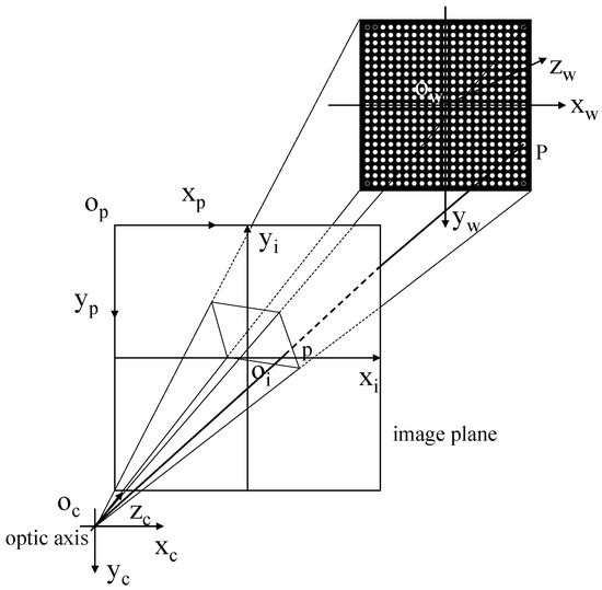
Figure 1.
Schematic diagram of the new cooperative target imaging.
Assuming there exists a point p on the image, in the pixel coordinate system, its x-axis value is denoted as u, and the y-axis value is denoted as v. Therefore, its pixel coordinates can be represented as , the 3D coordinates of the corresponding spatial point , and the chi-square expressions for both are . . Then, the projection relation between the two is shown in Equation (1).
where s is the scale factor; is the external reference matrix, which is used to transform between the world coordinate system and the camera coordinate system, where R is the rotation matrix, t is the translation vector, and the pose of the target is one-to-one with its external reference matrix. The camera’s internal reference matrix, K, is shown in Equation (2).
where represent the coordinates of the image’s principal points, , represent the pixel axis and focal length values in the direction of the axis, and is the tilt factor of the image element axis.
Since the world coordinate system is on the target scale now, the axis is perpendicular to the target coordinate, so the z-coordinates of the feature points will all be equal to 0. The three-dimensional coordinate point of P can be represented as and the corresponding chi-square coordinates are . Define the first column vector of the rotation matrix R is , which can be expressed by substituting it into Equation (3):
It is important for the feature points of the target itself to be all on the same spatial plane. When the camera captures the feature points, a homography transformation relationship exists between the spatial plane and the image plane, i.e., the spatial coordinates of the feature points can be transformed into pixel coordinates by a homography matrix. Let us define the homography matrix as H. At this point, H satisfies Equation (4).
Substituting into Equation (3), we obtain
which, due to the existence of scale invariance in the chi-square coordinates, yields an arbitrary scalar . At this point it follows that H is a matrix defined by , substituting into Equation (5), we have:
The rotation matrix R is an orthogonal matrix, their and are standard orthogonal bases, both mutually perpendicular and of modulus 1, i.e., satisfying and , which can be obtained by combining Equation (6):
Two basic constraints on the camera’s internal reference have thus been obtained. Let
where B is a symmetric matrix that can be expressed as a six-dimensional vector
Let the ith column vector of the homography matrix H be ; then, we have
However, the coefficient matrix of Equation (11) has only two rows, which is not enough to solve the 6-dimensional vector b. Therefore, we need to shoot n targets to obtain n single responsivity matrices and coefficient matrices with rows. When , then we can solve for the 6-dimensional vector b. That is, we need to obtain at least 3 pictures of the target to complete the calibration of the camera, and the total system of equations obtained at this time can be expressed as:
V is a matrix of coefficients.
At this point, Equation (12) is scale-equivalent, i.e., solving for b multiplied by any multiple is still the correct solution, so the matrix B consisting of b does not strictly satisfy , but rather there exists a scale factor that satisfies . By deduction, all camera parameters can be calculated from Equation (13).
Among them, .
3. Methods
3.1. Target Topology Design and Image Matching
Existing cooperative targets are mainly divided into checkerboard grid targets and circular targets. To further improve the accuracy of target feature point coordinate extraction and avoid the ambiguity caused by rotation, this paper combines the advantages of the two kinds of target markers and designs a new cooperative target marker, as shown in Figure 2a. It only consists of circles and rings as the target’s design pattern. The target’s approximate spatial pose is determined according to the special positional relationship of the five rings while avoiding the ambiguity caused by the target after 180-degree rotation. According to the application requirements, the target is easy to retrofit for use, the relative pose of the rings remains unchanged, and the corresponding sorting logic can be combined to be compatible with target feature points of different dimensions, as shown in Figure 2b, which can be changed to a feature point arrangement. To further improve the accuracy and increase the number of circles based on the limited space design, the experiments in this paper, all shown in Figure 2a, are used . The new type of cooperative target has the size of 220 mm × 220 mm.
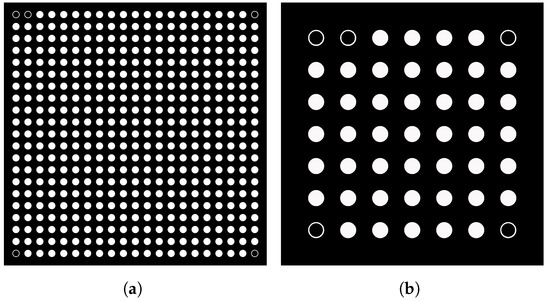
Figure 2.
Novel cooperative targets. (a) new co-operative targets, (b) new co-operative targets.
In the overall measurement system, feature point matching with its image is significant. According to the characteristics of the new type of target marker feature point sorting, this paper proposes an algorithm that can quickly and accurately match feature points with their images. The algorithm can accurately number the feature points on the target and the feature points in the picture and then correspond to them individually, providing an adequate data basis for the subsequent coordinate solving.
As in Figure 3, the feature points on the target mark are sorted and then connected two by two in order:
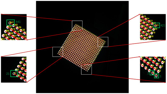
Figure 3.
Matching of feature points with corresponding image point images.
The sorting logic implemented is as follows:
- (1)
- The computer processes the image to obtain the coordinates of the feature points in the image plane , and the corresponding grey values of each feature point in the binarised image , .
- (2)
- Based on the new target’s unique circular feature point design, the grey value 255 is five particular circular coordinate points. As in Figure 3, the five particular coordinate points are recorded as Point 1, Point 2, Point 21, Point 421, and Point 441, and at this time, the ordering of the coordinates of the five particular feature points is unknown.
- (3)
- The points are processesd two by two to obtain the Euclidean distance; to meet the distance nearest condition of the two characteristics of the point—that is, Point 1 and Point 2, at this time only two relative relationships—the specific correspondence is unknown.
- (4)
- Points 1 and 2 define a straight line, and the closest point of the remaining 3 points to this line is Point 21.
- (5)
- Point 1 and 2 are each distanced from Point 21, the point closest to Point 21 is Point 2, and the point furthest away is Point 1.
- (6)
- The remaining two points are made as a line segment, and this segment’s midpoint is noted as Point Z. A vector is made from Point 1 to Point Z. Since the positive direction of the y-axis is downward in the pixel coordinate system if the point lies to the left of the vector, it is Point 441. Otherwise, the point is Point 421. At this point, the order of the coordinates of the feature points of the five particular circles is determined.
- (7)
- Point 1 and Point 421 are used to find a straight line, according to the perpendicular distance from the point to the straight line and the size of the space from Point 1 to obtain the correct order of the Point 1 and Point 421 columns of all the points as well as the correct order of Point 21 and Point 441 between the columns of all the facts on the order. The two columns of all the points correspond to each other, according to the corresponding two points to find a straight line, the closest vertical distance from the line, and according to the distance from Point 1 and Point 441, the size of the sheer length of the line to determine the correct order of all the points in each row. The proper ordering of the issues in each row will be combined to obtain the appropriate ordering of the coordinates of all 441 feature points.
Since the relative positional relationship of the points is used, the method is highly robust. It can still provide correct feature point ordering when the pose of the new cooperative target is highly variable after the sorting is completed. The specific row and column positions of the points in the coordinates of the feature points can be obtained after the sorting is completed.
3.2. Algorithms Related to Target Image Processing
3.2.1. Camera Self-Calibration
The sub-pixel coordinates of the feature points are the primary data for the whole pose measurement, which is mainly obtained by combining the pixel coordinate parameters on the image with the intrinsic parameters of the camera itself, so obtaining accurate camera parameters is crucial for the whole measurement system.
The traditional camera calibration method generally adopts Zhang’s calibration method, and the camera calibration target scale generally adopts a checkerboard target. However, after the relative pose relationship between the camera and the target changes, it will also cause a slight change in the camera parameters. This can be ignored in the usual measurement of low-precision requirements. Still, it is necessary to re-calibrate the camera for high-precision measurement. It is troublesome to recalibrate the camera every time the measurement target changes. To solve the above problems, combined with Zhang’s calibration method, the original checkerboard grid target is replaced with the existing new cooperative target. After the target is moved or the measurement pose is changed, it is only necessary to follow the operation procedure of Zhang’s calibration method to take several pictures of the new cooperative target in different poses. Then, the self-calibration of the camera can be completed.
Calibration step: after installing the new cooperative target and camera in a suitable pose, the new collective target is manipulated to transform the pose. After the change, the camera takes pictures and saves them, and after taking 15 or more photos, the feature points are extracted and sorted, and the camera parameters can be obtained through Equations (1)–(14). Figure 4a is the visual display centred on the camera, and Figure 4b is the visual display centred on the target. The three-coloured arrows indicate the pose of the camera relative to the target mark at this time; the centre of the three hands indicates the optical centre of the camera, the blue arrow indicates the pointing of the camera lens, the green arrow points to the top of the camera, and the red arrow points to the left side of the camera.
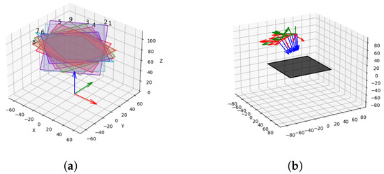
Figure 4.
Visual camera external reference. (a) Camera-centred, (b) target-centred.
3.2.2. Ellipse Fitting Based on the RANSAC Algorithm
In the final image-matching stage, model parameters must be estimated for the sample set obtained from coarse matching. However, due to image noise, etc., coarse matching based simply on the magnitude of the Euclidean spatial distances to find possible matches to the current point from the mapped set of points does not directly determine that these matches conform to the desired mapping model. In the ellipse fitting problem, this is manifested in the elimination of discrete or noisy points from a sample set in the ellipse fitting so that the elliptic equation obtained is more in line with reality compared to the elliptic model directly fitted with all the sample points, but it also further eliminates the error brought by the noise for the influence of the coordinate centre of the feature points to make the model parameter estimation to maintain a better robustness. Therefore, to better remove the mismatched points in the sample set, the RANSAC algorithm is introduced into the process of the least squares fitting ellipse through which the points with higher dispersion of the ellipse edges are removed to improve the accuracy of the ellipse centre further.
The RANSAC algorithm can divide all points into out-of-bounds and in-bounds points. The in-local points are the points whose distance to the model is less than a set threshold, and the out-local points are the points whose distance to the model is greater than the threshold, i.e., noise. Taking fitting an ellipse as an example, the number of iterations is set to 100, and the algorithm process is shown in Algorithm 1.
| Algorithm 1 Ellipse Fitting using RANSAC | |
| Input: Set of data points , number of iterations , fitting threshold | |
| Output: Best model parameters | |
| 1: | Best model parameters ← empty |
| 2: | Best model support count ← 0 |
| 3: | for to do |
| 4: | Randomly select the minimum required set of data points as the candidate set |
| 5: | Fit an ellipse model using , obtaining parameters |
| 6: | Current model support count ← 0 |
| 7: | for each data point in do |
| 8: | Calculate the distance from to the ellipse |
| 9: | if distance is less than then |
| 10: | Increment the current model support count |
| 11: | if current model support count > best model support count then |
| 12: | Update best model parameters and support count |
| 13: | end if |
| 14: | end if |
| 15: | end for |
| 16: | end for |
| 17: | Return Best model parameters |
Finally, by using the fitting results, the key parameters of the elliptic equation can be obtained, and the centre coordinates of the ellipse can be calculated. Consider the outer circle of the circular ring as an ellipse, and there are a total of 441 feature circles on the target. By repeating the above steps, all 441 centre points can be obtained.
3.2.3. Topology-Based Fitting for Intersection
In perspective projection, the coordinates of an object in the camera’s coordinate system and the coordinates of the object in the image plane of the object is a linear transformation relationship, i.e., where represents the coefficients of the linear transformation. It can be seen that the image formed by the perspective projection of a straight line in space is still a straight line. The straight line . The point of the line in the area is , both of which satisfy the relationship shown in Equation (15):
The coordinates of the feature points in a row or column of the target, which are arranged in a straight line, remain unchanged in the row and column arrangement after the target undergoes pose transformation. Based on this, the obtained sub-pixel coordinates are arranged in rows and columns with 21 rows and 21 columns. Each row and column contains 21 sub-pixel coordinates and 441 sub-pixel coordinates, i.e., the intersection points of all rows and columns. However, since the 21 coordinates of each row and each column are not exactly on a straight line, the optimal straight line formula can be obtained by least squares fitting, and the intersection coordinates of the 21 row and 21 column coordinates can be obtained again to obtain more accurate sub-pixel coordinates of the 441 feature points.
4. Results
To verify the feasibility of the algorithm and analyse the accuracy of the algorithm, the following experiments are carried out: the first group of experiments is a simulation-based camera calibration experiment, which is used to verify the superiority of the topology-based fitting intersection algorithm as well as the accuracy difference of the new type of directional targeting target compared with the traditional checkerboard targeting target in terms of the calibration of the camera parameters; the second group of experiments is the simulation experiment of the pose solving, which is used to verify the theoretical accuracy of the overall system in the absence of hardware errors; the third group is the actual shooting experiment of the pose solving.
4.1. Camera Calibration Simulation Experiment
Based on the 3ds Max platform, a set of simulation experimental systems is designed; its main function is to use the camera imaging principle without considering the lens aberration, image noise, mechanical errors generated during installation and mechanical errors in the plane movement to be measured, according to the input pose transformation value to be transformed from the zero-pose image to the image to be measured, to replace the actual painting, and by this paper’s method for camera. The camera is self-calibrated according to the method of this paper, and 20 images are simulated to prove the feasibility of the method of this paper by calculating the reprojection error value of each feature point in each image. In the simulation platform, the physical dimensions of the newly set target are 220 mm × 220 mm.
To verify the accuracy difference between the new directional target and the traditional checkerboard target in calibrating the camera parameters, and considering the potential ambiguity of the checkerboard target after a 180-degree rotation, a simulated checkerboard target with dimensions of specifications is generated. The physical size is 230 mm × 220 mm. Subsequently, 20 images are captured for camera calibration using the aforementioned simulation system, and the calibration results are calculated by the MATLAB Camera Calibration Toolbox.
The reprojection error values of each feature point in the 20 maps are expressed as Euclidean distances in pixels. There are 462 traditional checkerboard target feature points and 441 new directional target feature points. The experimental results are shown in Figure 5. The green line represents the reprojection error value corresponding to each point in the 20 images of the traditional chessboard target, and the dark green line is the average of the 20 error values; The blue line represents the reprojection error value corresponding to each point in the 20 images of the new target without fitting and intersecting points, and the dark blue line is the average of the 20 error values; The red line represents the reprojection error value corresponding to each point in the 20 images of the new target after fitting and intersecting points, and the dark red line is the average of the 20 error values.
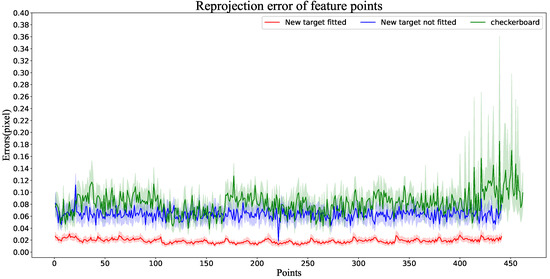
Figure 5.
Reprojection error of each feature point.
From the results shown in Figure 5, it can be seen that the reprojection error of the traditional checkerboard target is still larger than that of the new directional target without fitting the intersection points; after the intersection points are fitted to the feature points, the value of the reprojection error is further reduced, and the difference in the reprojection error between individual points is also further reduced.
4.2. Pose-Solving Simulation Experiment
Based on the above simulation platform, after obtaining the calibration results, the corresponding pictures are generated by simulation according to the pre-set completed angles. The simulation experiment is mainly divided into two parts. One is to detect the error of the system itself in four different pose situations; the other is to calculate the repeatability error of the system by subtracting the system error after obtaining the results.
To cover more pose angles and to demonstrate the measurement range of the system, four prominent cases of simulated curves were selected: a smaller angle of rotation in the positive direction, a smaller angle of rotation in the negative direction, a larger angle of rotation in the positive direction, and a larger angle of rotation in the negative direction. Fifteen diagrams were generated for each case simulation for calculation. The simulation results are shown in Figure 6, Figure 7, Figure 8 and Figure 9, respectively. The line chart above represents the pitch angle error value, the line chart below represents the roll angle error value, the green line represents the average error value of the attitude angle, and the red line represents the maximum error value of the attitude angle. The combination of the angle of the upper and lower line graphs corresponds to complete attitude angle errors of the simulation graph.
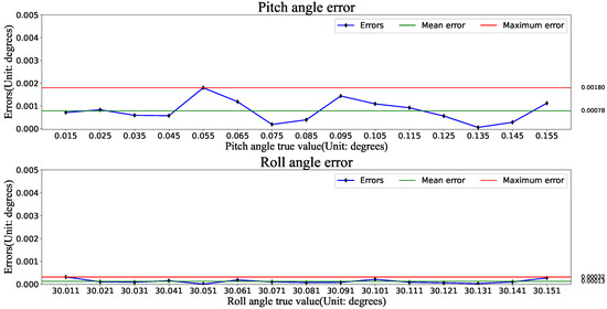
Figure 6.
Smaller angle of rotation in the positive direction.
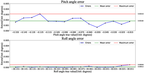
Figure 7.
Smaller angle of rotation in the negative direction.
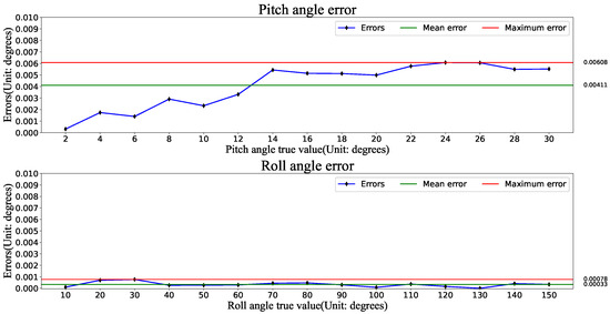
Figure 8.
Larger angle of rotation in the positive direction.
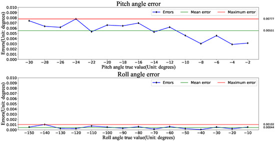
Figure 9.
Larger angle of rotation in the negative direction.
From the results shown in Figure 6, Figure 7, Figure 8 and Figure 9, it can be seen that after using this method, the measurement error of the tumbling angle perpendicular to the optical axis direction is 0.001° at the maximum, and the average error is 0.00044° at the maximum; the measurement error of the pitch angle is 0.008° at the maximum, and the average error is 0.00551° at the maximum. The measurement error of the roll angle is generally much smaller than that of the pitch angle. The accuracy is inversely proportional to the pitch angle, and the angular error in the roll direction is more stable.
To further simulate the stability of the system to solve the pose, the two perspectives of roll angle 10°, pitch angle 5° and roll angle −20°, pitch angle −10° were further selected, and 15 pictures were simulated to be generated for each pose, respectively. Their average error was used as the system error. The error of each image subtracted from the system error value was used as the error of the repeatability accuracy. The experimental results are shown in Figure 10 and Figure 11. The line chart above represents the pitch angle error value, the line chart below represents the roll angle error value, the green line represents the average error value of the attitude angle, and the red line represents the maximum error value of the attitude angle. The combination of the angle of the upper and lower line graphs corresponds to the complete attitude angle errors of the simulation graph.
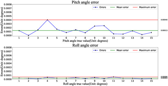
Figure 10.
Repeat accuracy error at 10° roll angle and 5° pitch angle.
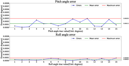
Figure 11.
Repeat accuracy error at roll angle −20° and pitch angle −10°.
From the results shown in Figure 10 and Figure 11, it can be seen that after using this method, the maximum error of repeated measurement of the tumble angle perpendicular to the direction of the optical axis is 0.00008°, and the average maximum mistake of repeated measurement is 0.00003°; the maximum error of repeated measurement of the pitch angle is 0.0004°, and the maximum average error of repeated measurement is 0.00013°. It can be analysed that the repeated size for a short period has a very small variation of error, and the error is randomly distributed.
From the above simulation experiments, the method can theoretically achieve a very high pose resolution accuracy, the measurement range is large, and the repeat measurement accuracy is very high. However, the algorithm still has a small error in the extraction of the ellipse centre coordinates, by which the simulated camera calibration parameters obtained also have a certain error, which finally leads to the simulation results and the actual pose still having a certain error.
4.3. Pose Solving Practical Filming Experiments
The experimental system of monocular vision pose measurement built in the actual scene is shown in Figure 12, and the testing platform is mainly composed of a two-axis rotary table and a camera. The model of the two-axis rotary table is PTU-E46-17P70T, the accuracy of the pitch axis is up to 0.003 degrees, and the accuracy of the tumble axis is up to 0.013 degrees. The camera chosen is a Basler ace2 a2A2840-48ucBAS, equipped with a Sony IMX546 CMOS chip, with a frame rate of 48 fps, a resolution of 8 megapixels, and horizontal and vertical pixel dimensions of 2.74 μm. The lens of choice is the Ricoh Lens FL-CC0616A-2M, with a focal length of 6.0 mm and an aperture of F1.4-F16.0.
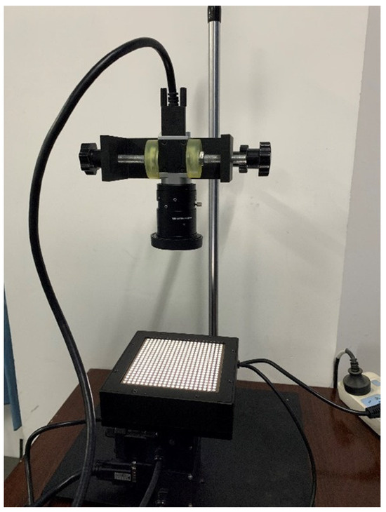
Figure 12.
Experimental system for monocular vision pose measurement.
According to the settings of the simulation experiment, the pictures are taken with the same pose. The actual shooting pose solution results are shown in Figure 13, Figure 14, Figure 15 and Figure 16. The line chart above represents the pitch angle error value, the line chart below represents the roll angle error value, the green line represents the average error value of the attitude angle, and the red line represents the maximum error value of the attitude angle. The combination of the angle of the upper and lower line graphs corresponds to complete attitude angle errors of the actual shooting graph.
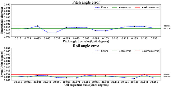
Figure 13.
Smaller angle of rotation in the positive direction..
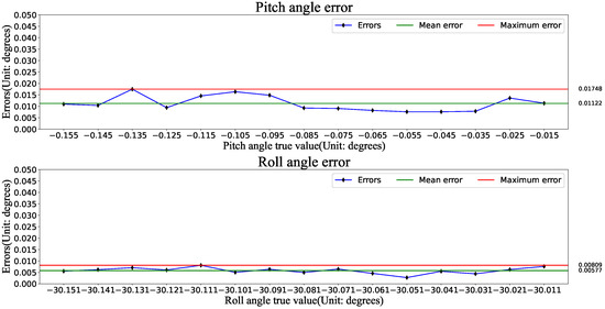
Figure 14.
Smaller angle of rotation in the negative direction.
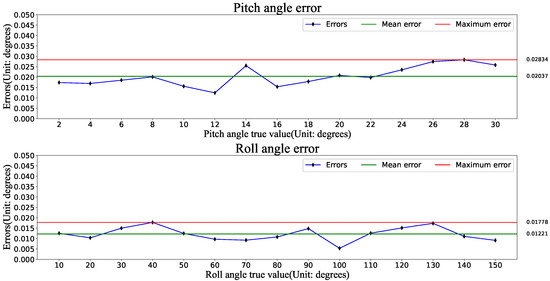
Figure 15.
Larger angle of rotation in the positive direction.
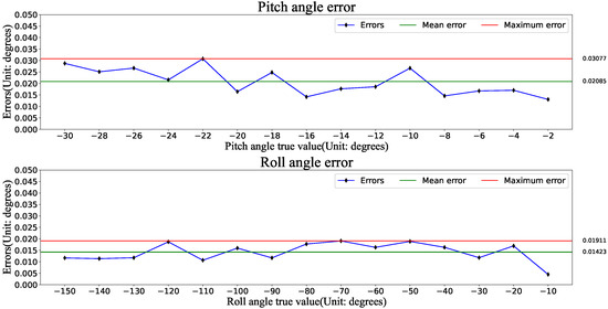
Figure 16.
Larger angle of rotation in the negative direction.
From the results shown in Figure 13, Figure 14, Figure 15 and Figure 16, it can be seen that using this method after considering the camera imaging noise and the overall mechanical error, the measurement error of the tumbling angle perpendicular to the optical axis direction is 0.01911° at most, and the average error is 0.01423° at most; the measurement error of the pitch angle is 0.03077° at most, and the average error is 0.02085° at most. The measurement error of the roll angle is generally much more minor than the pitch angle’s, the accuracy is inversely proportional to the pitch angle, and the angular error in the roll direction is more stable. In addition to the large difference in accuracy, the change rule of the error is consistent with the simulation results.
Based on the simulation experiments, the two poses of roll angle 10°, pitch angle 5°, and roll angle −20 °, pitch angle −10 ° were further selected, and 15 pictures were taken for each pose. Their average error was taken as a systematic error. The error of each image subtracted from the value of the systematic error was taken as the error of the repeatability accuracy. The experimental results are shown in Figure 17 and Figure 18. The line chart above represents the pitch angle error value, the line chart below represents the roll angle error value, the green line represents the average error value of the attitude angle, and the red line represents the maximum error value of the attitude angle. The combination of the angle of the upper and lower line graphs corresponds to the complete attitude angle errors of the actual shooting graph.
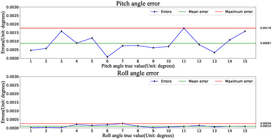
Figure 17.
Repeat accuracy error at 10° roll angle and 5° pitch angle.
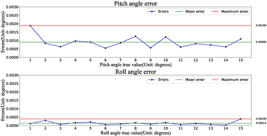
Figure 18.
Repeat accuracy error at roll angle −20° and pitch angle −10°.
The results in Figure 17 and Figure 18 show that the maximum error of repeated measurement of the tumble angle perpendicular to the direction of the optical axis is 0.00039°. The average maximum mistake of repeated measurement is 0.00014°, the maximum error of repeated measurement of the pitch angle is 0.0004°, and the average maximum mistake of repeated measurement is 0.0009°. The short-time repeated measurements have very small changes in the errors, and the errors are randomly distributed.
In real-world scenarios, due to factors such as environmental temperature, camera noise, and errors in the mechanical turntable, there are significant differences in accuracy compared to simulation results. The pose variation range selected in Figure 13 and Figure 14 is extremely small, making it difficult to discern the distribution of errors. Figure 15 and Figure 16 are influenced by external factors, resulting in less obvious error distributions. However, overall, the conclusions obtained from actual shooting are consistent with the simulation results. The angle error in pitch direction is inversely proportional to the pitch angle, while the angle error in the roll direction is relatively stable. The repeated measurement errors exhibit a state of random distribution.
5. Conclusions
Monocular vision measurement has been one of the hotspots in the industry due to the advantages of simple equipment and few operation steps. A pose measurement method based on machine vision and a new type of directional target is proposed to achieve high-precision measurement of object pose. The new directional target is designed and manufactured, and the object-matching algorithm for the target is implemented; the high-precision calibration of the camera is realised based on the target; various algorithms are introduced to improve the accuracy of the coordinates of the feature points and further reduce the error of the pose calculation.
Several experiments show that the camera calibration parameters obtained using this target are higher than those of the traditional checkerboard target; calculating the object’s pose can be achieved with high accuracy. The system has a simple structure, fast speed, high precision and stability.
The significance of the pose measurement method proposed in this paper is that the self-calibration of the camera can be realised without the help of external equipment, and then the high-precision pose data of the object to be measured can be obtained. The method in this paper can make the target for arbitrary installation, which further reduces the application requirements of the vision measurement method, simplifies the measurement steps while ensuring measurement accuracy, and broadens the application scope of monocular vision measurement.
Author Contributions
Conceptualisation, D.S., X.W. and Z.Z.; methodology, Z.Z. and X.W.; software, Z.Z.; validation, D.S., X.W. and Z.Z.; formal analysis, Z.Z. and X.W.; investigation, Z.Z.; resources, D.S. and X.W.; data curation, Z.Z.; writing—original draft preparation, Z.Z.; writing—review and editing, X.W. and P.Z.; visualisation, Z.Z.; supervision, D.S., X.W. and P.Z.; project administration, D.S.; funding acquisition, D.S. All authors have read and agreed to the published version of the manuscript.
Funding
This work is supported by the Key R&D Plan of Shandong Province (Major Science and Technology Innovation Project) No. 2023CXGC010701; in part by the Project of 20 Policies of Facilitate Scientific Research in Jinan Colleges No. 2019GXRC063; in part by the Project of Shandong Provincial Major Scientific and Technological Innovation, grant No. 2019JZZY010444, No. 2019TSLH0315; and in part by the Natural Science Foundation of Shandong Province, grant No. ZR2020MF138.
Data Availability Statement
Data available on request due to privacy. The data presented in this study are available on request from the corresponding author.
Conflicts of Interest
The authors declare no conflicts of interest.
References
- García-Mateos, G.; Hernández-Hernández, J.L.; Escarabajal-Henarejos, D.; Jaén-Terrones, S.; Molina-Martínez, J.M. Study and comparison of color models for automatic image analysis in irrigation management applications. Agric. Water Manag. 2015, 151, 158–166. [Google Scholar] [CrossRef]
- Hernández-Hernández, J.L.; García-Mateos, G.; González-Esquiva, J.M.; Escarabajal-Henarejos, D.; Ruiz-Canales, A.; Molina-Martínez, J.M. Optimal color space selection method for plant/soil segmentation in agriculture. Comput. Electron. Agric. 2016, 122, 124–132. [Google Scholar] [CrossRef]
- Andrzej, S. Geometry and resolution in triangulation vision systems. In Proceedings of the Photonics Applications in Astronomy Communications, Industry, and High Energy Physics Experiments, Wilga, Poland, 31 August–2 September 2020; Volume 11581, p. 115810Y. [Google Scholar]
- He, W.; Zhang, A.; Wang, P. Weld Cross-Section Profile Fitting and Geometric Dimension Measurement Method Based on Machine Vision. Appl. Sci. 2023, 13, 4455. [Google Scholar] [CrossRef]
- Li, R.; Fu, J.; Zhai, F.; Huang, Z. Recognition and Pose Estimation Method for Stacked Sheet Metal Parts. Appl. Sci. 2023, 13, 4212. [Google Scholar] [CrossRef]
- Su, J.D.; Duan, X.S.; Qi, X.H. Planar target pose measurement and its simulation based on monocular vision. Firepower Command. Control 2018, 7, 160–165. [Google Scholar]
- Su, J.D.; Qi, X.H.; Duan, X.S. Planar pose measurement method based on monocular vision and checkerboard target. J. Opt. 2017, 8, 218–228. [Google Scholar]
- Chen, Z.K.; Xu, A.; Wang, F.B.; Wang, Y. Target pose measurement method based on monocular vision and circular structured light. Appl. Opt. 2016, 5, 680–685. [Google Scholar]
- Sun, P.F.; Zhang, Q.Z.; Li, W.Q.; Wang, P.; Sun, C. Monocular multi-angle spatial point coordinate measurement method. J. Instrum. 2014, 12, 2801–2807. [Google Scholar]
- Richard, H.; Andrew, Z. Multiple View Geometry in Computer Vision, 2nd ed.; Cambridge University Press: Cambridge, UK, 2004. [Google Scholar]
- Pan, H.Z.; Huang, J.Y.; Qin, S.Y. High accurate estimation of relative pose of cooperative space targets based on measurement of monocular vision imaging. Optik 2014, 13, 3127–3133. [Google Scholar] [CrossRef]
- Li, W.; Ma, X.; Jia, Z.Y.; Zhang, Y.; Li, X. Position and attitude measurement of high-speed isolates for hypersonic facilities. Measurement 2015, 62, 63–73. [Google Scholar] [CrossRef]
- Prasad, D.K.; Leung, M.K.H.; Cho, S.Y. Edge curvature and convexity based ellipse detection method. Pattern Recogn 2012, 45, 3204–3221. [Google Scholar] [CrossRef]
- Chia, A.Y.S.; Rahardja, S.; Rajan, D.; Leung, M.K.H. A split and merge based ellipse detector with self-correcting capability. IEEE Trans. Image Process 2011, 20, 1991–2006. [Google Scholar] [CrossRef] [PubMed]
- Chen, X.Y.; Hu, Y.; Ma, Z.; Yu, S.H.H.; Chen, Y.Q. The location and identification of concentric circles in automatic camera calibration. Opt. Laser Technol. 2013, 54, 185–190. [Google Scholar] [CrossRef]
- Cui, J.S.; Huo, J.; Liu, T.; Yang, M. The high precision positioning algorithm of circular landmark centre in visual measurement. Optik 2014, 125, 6570–6575. [Google Scholar] [CrossRef]
- Cui, J.; Huo, J.; Yang, M. The circular mark projection error compensation in camera calibration. Optik 2015, 126, 2458–2463. [Google Scholar] [CrossRef]
- Li, J.L.; Zhang, D.W. Camera calibration with a near-parallel imaging system based on geometric moments. Opt. Eng. 2011, 50, 68. [Google Scholar]
- Wang, Y.; Yuan, F.; Jiang, H.; Hu, Y. Novel camera calibration based on cooperative target in attitude measurement. Optik 2016, 127, 10457–10466. [Google Scholar] [CrossRef]
- Xu, S.Y.; Zhu, L. A novel planar calibration method using the iterative correction of control points information. Optik 2013, 124, 5930–5936. [Google Scholar] [CrossRef]
Disclaimer/Publisher’s Note: The statements, opinions and data contained in all publications are solely those of the individual author(s) and contributor(s) and not of MDPI and/or the editor(s). MDPI and/or the editor(s) disclaim responsibility for any injury to people or property resulting from any ideas, methods, instructions or products referred to in the content. |
© 2024 by the authors. Licensee MDPI, Basel, Switzerland. This article is an open access article distributed under the terms and conditions of the Creative Commons Attribution (CC BY) license (https://creativecommons.org/licenses/by/4.0/).