Enhancing Dynagraph Card Classification in Pumping Systems Using Transfer Learning and the Swin Transformer Model

Featured Application

The developed prototype provides a more efficient and accurate solution for classifying dynagraph cards, meeting the requirements of oil field operations and enhancing economic benefits and work efficiency.

Abstract

The dynagraph card plays a crucial role in evaluating oilfield pumping systems’ performance. Nevertheless, classifying dynagraph cards can be quite difficult because certain operating conditions may exhibit similar patterns. Conventional classification approaches mainly involve labor-intensive manual analysis of these cards, leading to subjectivity, prolonged processing times, and vulnerability to human prejudices. In response to this challenge, our study introduces a novel approach that leverages transfer learning and the Swin Transformer model for classifying dynagraph cards across various operating conditions in rod pumping systems. Initially, the Swin Transformer model undergoes pre-training using the ImageNet-22k dataset. Subsequently, we fine-tune the model’s weights using actual dynagraph card datasets, facilitating direct classification analysis with dynagraph cards as input variables. The adoption of transfer learning significantly reduces the training time while enhancing the accuracy of condition diagnosis. To assess the effectiveness of our proposed method, we conducted a comparative evaluation against conventional models like ResNet50, DenseNet121, LeNet, and ViT. The findings demonstrate that our approach outperforms other methods, achieving an accuracy of 96%, thereby improving classification accuracy by 3–4%. Therefore, our approach, based on transfer learning and the Swin Transformer model, provides a better solution for practical problems involving similar dynagraph cards. It meets the requirements of oil field operations, enhancing economic benefits and work efficiency.

1. Introduction

In recent years, as one of the crucial pieces of equipment in the field of oil extraction, the pumping unit has played a key role in improving oil field recovery rates and enhancing production efficiency. To ensure the smooth operation of the pumping unit and minimize the risk of equipment failures, accurate and timely diagnosis is of paramount importance. Dynagraph cards, as a commonly used diagnostic tool, provide valuable information about the operating condition and performance of the pumping unit.

However, traditional methods for diagnosing pumping unit dynagraph cards are limited by manual analysis and domain expertise. Manual analysis requires a significant amount of time and effort, and is prone to subjective biases, leading to inconsistent and inaccurate diagnostic results [1]. In recent years, there have been remarkable advancements in the field of diagnosing pumping unit dynagraph cards, primarily through the adoption of machine learning techniques. These methods have been developed to address the challenges associated with manual analysis and the classification of dynagraph cards. As a result, machine-learning-based approaches have shown great promise in improving the accuracy, efficiency, and objectivity of dynagraph card diagnosis.

The development of dynagraph card diagnostic methods can be summarized as follows. Initially, expert diagnosis played a crucial role in dynagraph card diagnostics, relying on the extensive work experience and domain knowledge of oilfield engineering experts. By manually analyzing and interpreting dynagraph cards, experts could diagnose pump failures and provide corresponding solutions. This method relied on experts’ accurate understanding of dynagraph card features and patterns to infer pump issues. With the rise of machine learning, statistical and pattern-recognition-based machine learning methods were applied to pump failure diagnosis. Tian proposed a fault detection method employing support vector machines (SVM) and genetic algorithm optimization for accurate fault diagnosis based on pump fault information in 2007 [2]. Their method demonstrated high feasibility and effectiveness through experimental results. Li suggested a curve moments and PSO-SVM method to diagnose downhole conditions of pumping wells, achieving automated identification, feature parameter extraction, and pattern classification from dynagraph cards in 2013 [3]. Their approach exhibited excellent classification performance. With the advancement of deep learning, significant breakthroughs have been made in dynagraph card diagnostics. He presented a combination of convolutional neural networks (CNN) and long short-term memory (LSTM) networks for diagnosing gradual faults in 2019 [4]. By extracting multi-level abstract features and employing LSTM for sequence recognition, the method surpassed traditional mathematical models in diagnostic accuracy. Furthermore, the application of CNN-based image recognition techniques by Zhou enabled the diagnosis of oil well pumping unit failures through power card curve analysis [5]. This method showed high accuracy and practicality, making it a feasible approach for leveraging oilfield data assets. Despite the improvements in deep learning models, the small sample characteristics of dynagraph card data presented challenges when using large models like AlexNet and VGG in 2019. To address this, Cheng proposed an automatic recognition method based on transfer learning and support vector machines (SVM), utilizing a large amount of collected dynagraph card data from sensors for more efficient pumping system operating state recognition in 2020 [6]. Representative features of dynagraph cards were automatically extracted using transfer learning based on AlexNet. Combined with the extracted features, an SVM method based on error-correcting output codes (ECOC) was designed to identify the operating states of the pumping system, enhancing the accuracy and efficiency of fault diagnosis. Experimental results demonstrated the reduction in manual labor and improved the identification accuracy achieved by this method. With the continuous development of deep learning, Wibawa utilized self-supervised learning methods to classify dynagraph cards and improve the accuracy of performance monitoring for pumping systems by constructing deep learning models using unlabeled data in 2023 [7]. Results showed that, compared to ImageNet models, the AlexNet model based on pretext-invariant representation learning (PIRL) and jigsaw pre-training methods achieved a 6% performance improvement when using pre-trained models. Further fine-tuning with labeled data resulted in a model accuracy of 93%. With the outstanding performance of vision transformers in computer vision tasks, Zhang proposed a transfer-learning-based method using the ViT model for diagnosing conditions of rod pumping systems in 2023 [8]. The model showed excellent performance in practical production, achieving a 2% higher accuracy compared to traditional CNN models.

In the realm of deep learning, the transformer model, originally renowned for its success in natural language processing (NLP), has emerged as the preferred standard model. Additionally, the vision transformer model has exhibited remarkable capabilities in addressing computer vision tasks, as demonstrated in the study conducted by Dosovitskiy [9]. Recently, building on the achievements of the vision transformer model, the Swin Transformer has emerged as an innovative transformer model that introduces cross-window interaction and hierarchical feature representation, further improving the effectiveness of image understanding and analysis in 2021 [10]. This makes the Swin Transformer a powerful tool for handling dynagraph card diagnostic problems in pumping units.

However, for a pre-trained model, its predictive performance is limited if transfer learning is not employed. During the pre-training phase, large-scale datasets such as ImageNet-22k are utilized to provide rich image information, enabling the model to learn more generalized and abstract feature representations in advance. Subsequently, transfer learning is applied through fine-tuning on a small dataset (the oilfield dynagraph card dataset). Results have demonstrated that after pre-training with transfer learning, training the model with a smaller dataset of dynagraph cards can achieve an accuracy improvement of 3% to 4% compared to pre-training models such as traditional CNN models and ViT models. This underscores the feasibility of this approach in dynagraph card diagnostics.

Our research contributes in the following aspects: (1) The study proposes a novel approach that combines transfer learning with the Swin Transformer model for classifying dynagraph cards in rod pumping systems. (2) This innovative method addresses challenges in traditional manual analysis, providing a more efficient and accurate solution for diagnosing pump conditions. Leveraging transfer learning and the Swin Transformer model, it outperforms traditional methods such as ResNet50, DenseNet121, LeNet, and ViT. The research results demonstrate a significant improvement in classification accuracy, reaching 96%, surpassing other models, and showcasing the effectiveness of the introduced methodology. (3) The enhanced accuracy is crucial for reliable condition diagnosis in oilfield operations, contributing to increased economic benefits and overall work efficiency.

This paper aims to address the problem of dynagraph card diagnostics in pumping units by applying the Swin Transformer and transfer learning methods. Section 2 provides an introduction to the theoretical knowledge of pumping units and common types of dynagraph card faults. Section 3 presents a detailed description of the structures and parameters of two transformer models, namely ViT and Swin Transformer. Section 4 of the paper encompasses the following aspects: the dataset employed in the experiments, the experimental procedure, a comparative analysis of the results, and validation of the experimental findings. Lastly, the paper concludes in Section 5.

2. Materials and Methods

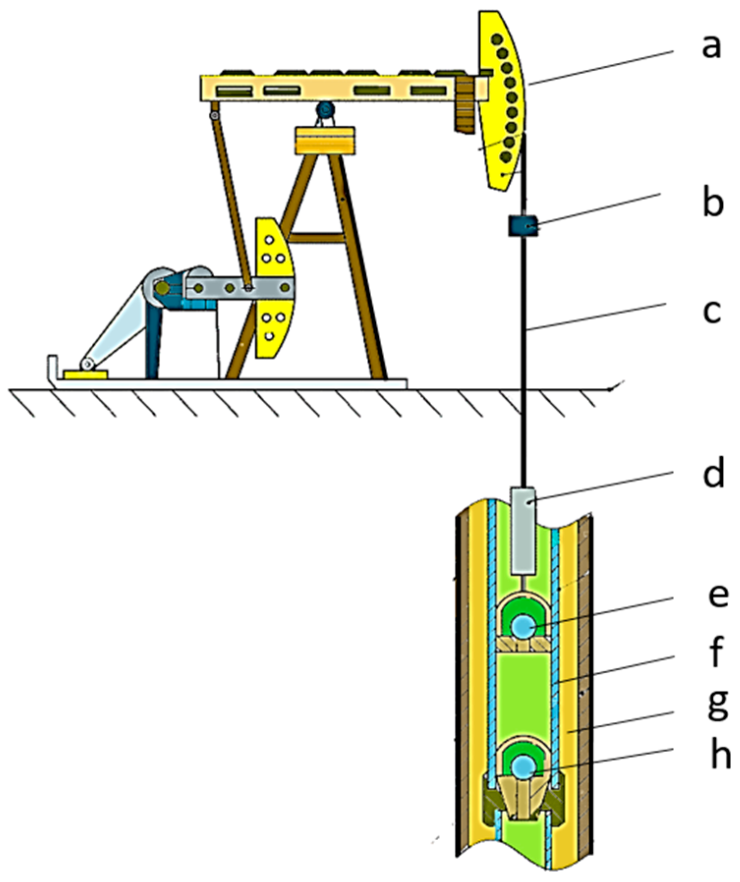
2.1. The Principle of Oil Extraction in a Pumping Unit

The pumping unit achieves oil extraction through the coordinated operation of the prime mover, sucker rod, and pump [11]. Any malfunction in these components will cause variations in the dynagraph card curve, making it meaningful to have an understanding of the working principles of the pumping equipment for dynagraph card classification.

A typical beam pumping system, which is the mainstream sucker rod pumping system, consists of three main components [12]. Firstly, there is the surface unit of the pumping unit, which is connected to a high-power prime mover. It includes components such as a gearbox, electric motor, connecting rod, walking beam, and crank, providing power for the system [13]. Secondly, there is the sucker rod, which connects to the pumping unit and the downhole pump, responsible for transmitting power. The sucker rod drives the pump to perform oil extraction and plays a vital role in the pumping process. Lastly, there is the downhole pump, which receives power and drives the pump to perform oil extraction. It mainly consists of components such as a pump barrel, valve, and plunger [14].

Through the power transmitted by the pumping unit, the sucker rod undergoes a continuous reciprocating motion, creating a stroke that causes the pump barrel to move up and down. During the upward stroke, the fluid column’s resistance forces the traveling valve in the pump barrel to close, while the hydraulic pressure of the fluid column opens the standing valve, allowing crude oil to be collected into the pump barrel [15]. Conversely, during the downward stroke, the force on the fluid column reverses, leading to the closure of the standing valve and the opening of the traveling valve. This allows the crude oil to be pumped out of the pump barrel and into the production tubing for collection. The uninterrupted movement of the sucker rod ensures a constant transportation of fluid from the wellbore into the pump barrel, thus completing the oil extraction process. The structure of a pumping unit well is depicted in Figure 1.

From the above oil extraction process, it is evident that the pump and sucker rod are critical components that work underground and are prone to failure. During the pumping process, the sucker rod is influenced by the up and down loads, which can result in a wavy pattern in the dynagraph card curve. Additionally, the inertia load can cause a clockwise rotation in the dynagraph card, and the opening and closing of valves can affect stroke losses. Therefore, the sucker rod is susceptible to failures such as bending, deformation, or even fracture under different loads. The traveling valve and standing valve of the pump constantly open and close to collect crude oil, but they may experience failures due to impurities in the oil or limitations in the lifespan of valve connections.

To quickly and accurately locate the faults in the pumping unit, it is essential to professionally collect dynagraph card data [16]. The dynagraph card describes the displacement and load conditions of the sucker rod, thus assisting in analyzing the working state of the pumping unit and identifying potential faults. Through an analysis of the dynagraph card, faults can be promptly identified, and corresponding maintenance measures can be taken to improve the operational efficiency and reliability of the pumping unit.

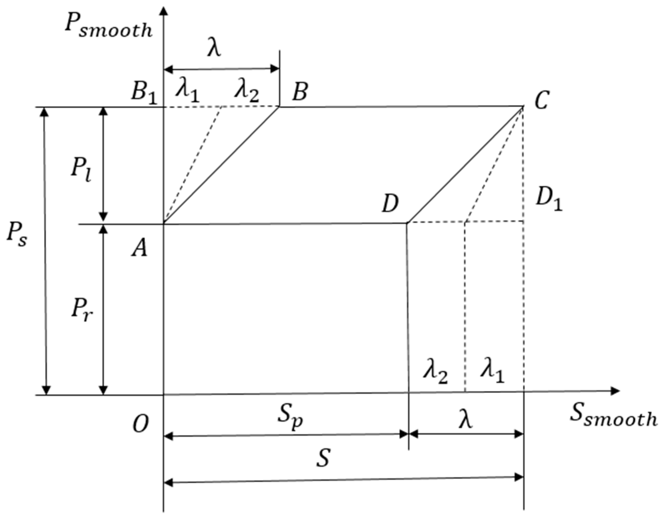
2.2. Theoretical Analysis of the Dynagraph Card

Figure 2 illustrates a theoretical pumping unit dynagraph card [17], depicting the displacement of the smooth rod of the pumping unit along the x-axis and representing the load on the smooth rod along the y-axis.

In Figure 2, S_smooth represents the stroke length, S_p denotes the piston stroke, P_r represents the mass of the sucker rod in the oil, $P_l$ indicates the mass of the fluid column above the pump, $P_s$ represents the static load borne by the smooth rod, ${\lambda }_1$ represents the elongation or contraction of the sucker rod, ${\lambda }_2$ represents the elongation or contraction of the tubing, and $\lambda$ represents the stroke loss, which is equal to the sum of ${\lambda }_1$ and ${\lambda }_2$.

In an ideal scenario, the dynagraph card of a pumping unit takes the form of a parallelogram, ABCD. The ABC segment represents the variation in static load during the upstroke process of the pump. During this phase, the load gradually transfers from the fluid column above the pump to the plunger, causing it to remain stationary without any actual displacement. Consequently, both the traveling valve and the standing valve remain closed. At point B, all the fluid column loads are transferred to the plunger, and the extension of the sucker rod and tubing also reaches its limit. Beyond point B, the relative position between the plunger and the pump barrel begins to change. As the pressure inside the pump becomes lower than the submergence pressure, the standing valve opens, and the pump initiates fluid intake. The BC segment on the dynagraph card represents the process of the pump suctioning well fluid, with the traveling valve remaining closed. The CDA segment on the card illustrates the variation in static load during the downstroke process of the pump. During the CD section, the load gradually unloads, and there is no relative displacement between the plunger and the pump barrel. The traveling valve remains closed throughout the unloading process, until reaching point D. At this point, the compression of the sucker rod and tubing also concludes. From point D back to point A, the plunger undergoes actual displacement, and the standing valve closes. Simultaneously, the traveling valve opens to discharge the fluid from the pump barrel.

2.3. Analysis of Dynagraph Cards under Different Operating Conditions

The analysis of dynagraph cards under different operating conditions can help us understand potential issues and faults in the pumping unit system [18]. Here is an analysis of dynagraph cards under several common operating conditions:

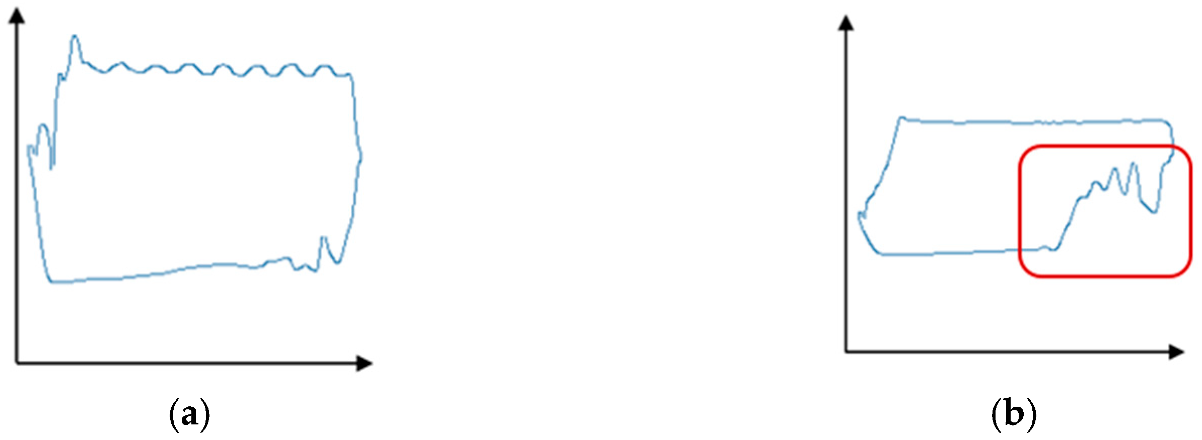
• Normal Pump Operation: The dynagraph card shows a regular pattern without any anomalies, as depicted in Figure 3a.
• Fluid Pound [19]: Fluid pound refers to the impact force generated during the pumping process due to the interaction between the pump barrel and the gas–liquid drive system. Fluid pound is characterized by sudden spikes and steep drops in the dynagraph card. It is often caused by factors such as the excessive downward speed of the pump rod, seal failure between the pump rod and the fluid, and unstable motion of the fluid column (Figure 3b).
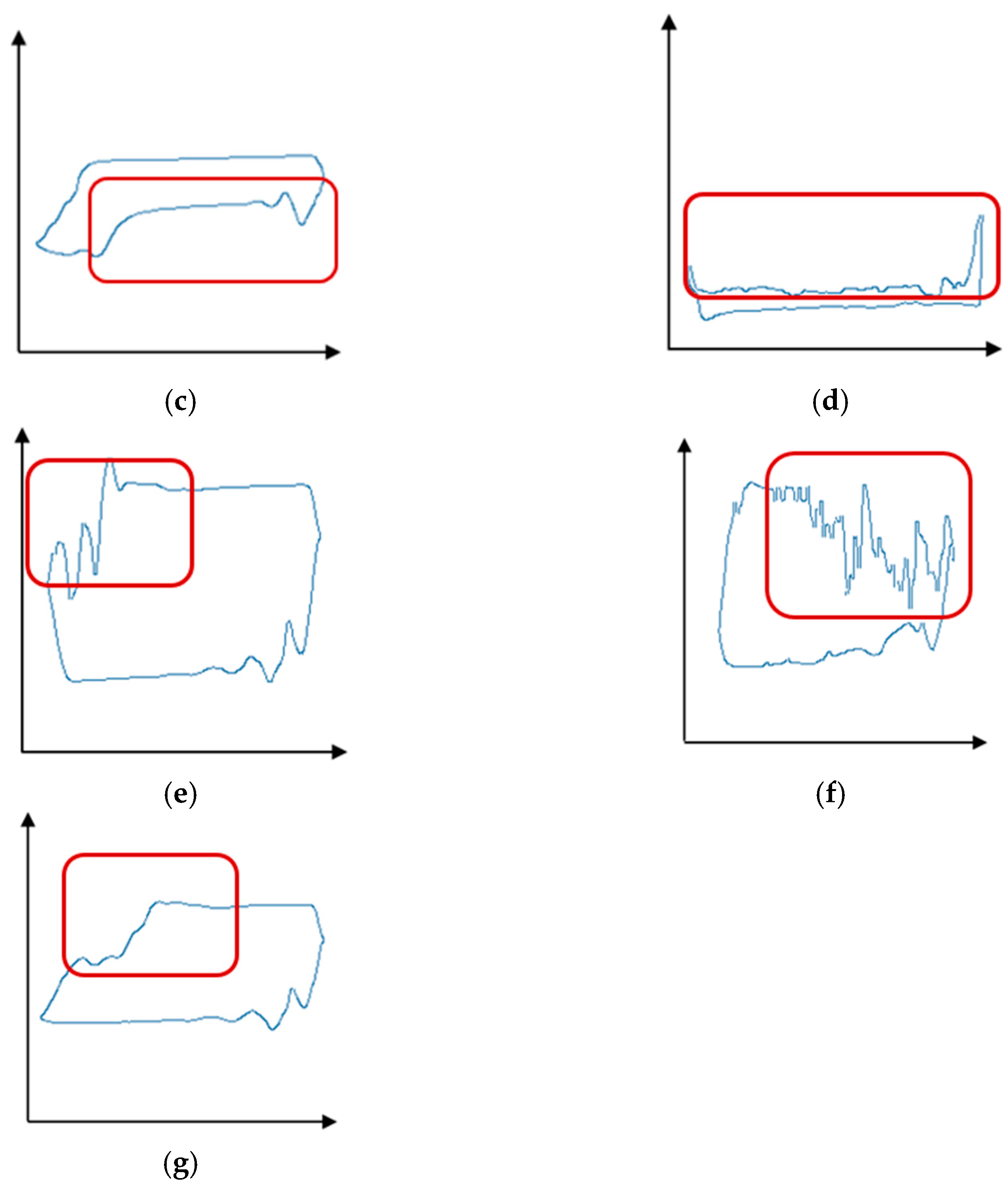
• Gas Interference: The presence of gas has a significant impact on pump operation [20]. In the dynagraph card, gas interference is indicated by compression areas during the upstroke and downstroke of the pump, resulting in relatively smooth curve shapes. Gas interference is typically caused by factors such as gas production in the well, gas accumulation between the pump rod and the fluid, and failure of the gas–liquid drive system (Figure 3c).
• Gas Lock [21]: Gas lock refers to the accumulation of gas in the lower section of the pump rod or at the bottom of the well, creating an obstruction that prevents the fluid from entering the pump rod completely and hinders the downward motion of the pump rod. This condition is identifiable on the dynagraph card by an extended compression area during the downward stroke of the pump rod, represented by a relatively flat waveform. Gas lock is often caused by factors such as excessive gas production in the well, declining fluid level, and poor sealing of the pump rod (Figure 3d).
• Delayed Closure of the Traveling Valve [22]: Delayed closure of the traveling valve refers to the phenomenon where the traveling valve in the pump closes with a delay during the upstroke of the pump rod. In the dynagraph card, the delayed closure of the traveling valve results in an increase in the downward speed of the pump rod, leading to an accelerated descent and steeper slope during the downward stage (Figure 3e).
• Pump Barrel Slippage: Pump barrel slippage occurs when the pump barrel becomes dislodged and separates from the pump rod [23]. In the dynagraph card, pump barrel slippage is indicated by a sudden decrease in the slope during the descent stage, resulting in a smoother curve waveform. Pump barrel slippage is typically caused by factors such as poor installation of the pump barrel and wear of the pump barrel (Figure 3f).
• Fluid Pound and Delayed Closure of the Traveling Valve: The occurrence of both fluid pound and delayed closure of the traveling valve has an impact on the normal operation of the pump. Fluid pound can lead to damage to the pump rod and other components, while the delayed closure of the traveling valve can increase the upward speed of the pump rod, resulting in increased friction between the pump rod and the wellbore and affecting the stability of the pump rod’s operation (Figure 3g).

3. Correlation Algorithm

With the rapid advancements in technology, various convolutional neural network (CNN) frameworks [24] have emerged, including ResNet, DenseNet, and LeNet, which have become prevalent in the computer vision field, especially for dynagraph card diagnostics, showing promising results.

However, CNNs do have certain limitations [25]. First, they primarily focus on local features and typically use a sliding window approach to process images, limiting their ability to capture global information. Second, the convolution process may lead to the loss of valuable information. Third, due to the encapsulated nature of feature extraction, it becomes challenging to enhance the model effectively. Finally, CNNs can act as black boxes with limited interpretability.

In natural language processing (NLP) [26], the transformer model has become the preferred choice. Despite this, CNNs continue to dominate the computer vision domain. Taking inspiration from the success of transformers in NLP, the Google team made an attempt to directly apply the transformer to image analysis with minimal modifications, giving rise to the vision transformer (ViT) model [9]. ViT has shown remarkable performance in image classification tasks, particularly excelling in handling global context and large-scale image datasets and offering improved interpretability [27]. The introduction of the self-attention mechanism has brought innovative ideas and methods to image classification, opening up new avenues for advancements in computer vision [28].

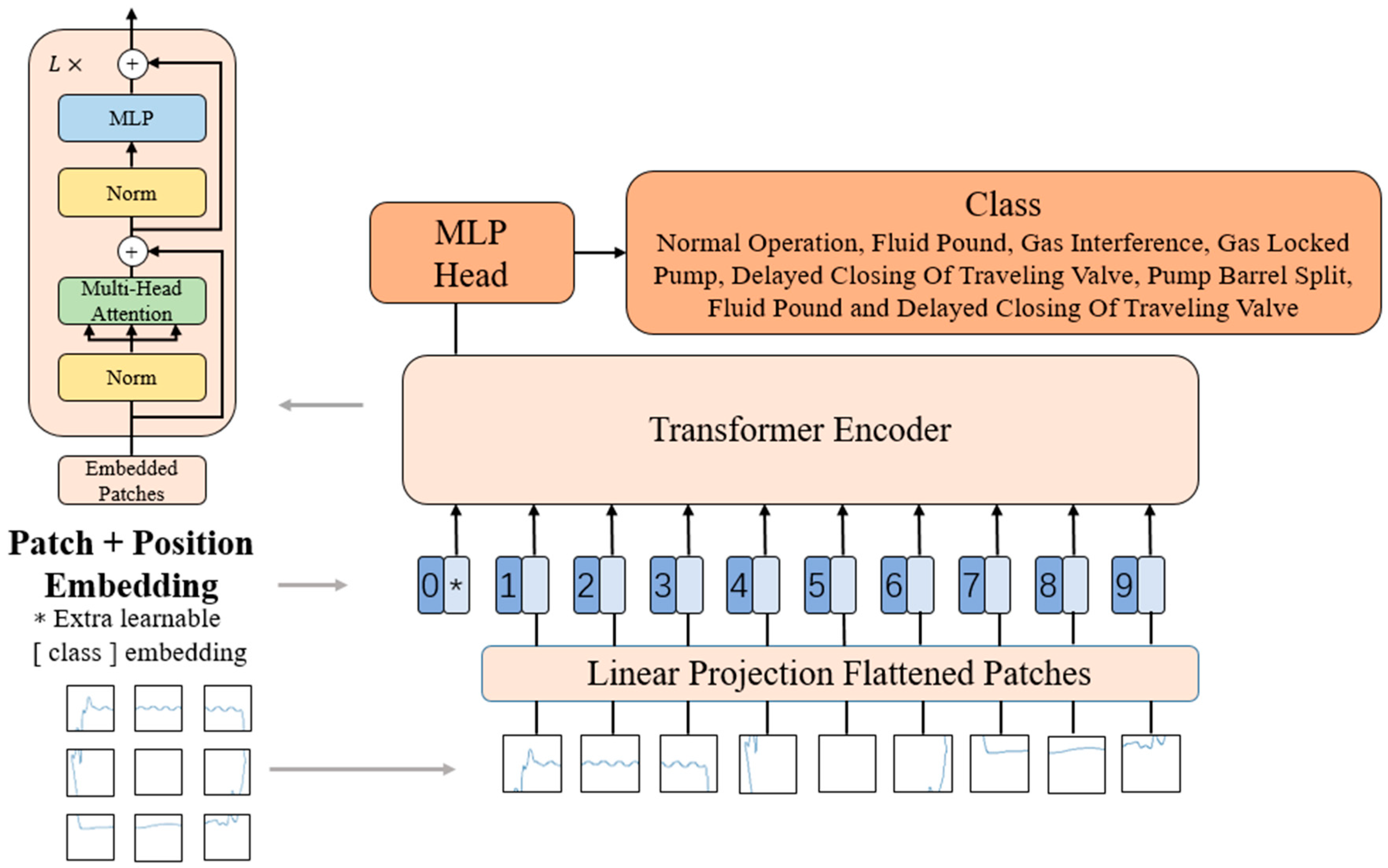
3.1. Vision Transformer

The Google team introduced the vision transformer (ViT) model in 2021, aiming to leverage the transformer’s capabilities for image classification tasks [29]. While previous research had explored applying transformers to visual tasks, ViT stands out as a significant milestone in the field of computer vision due to its simplicity, impressive performance, and scalability (larger models lead to better results). The release of ViT has triggered a surge of interest in transformer-based approaches for various visual tasks, including object detection and image generation. Figure 4 shows a visual representation of the ViT architecture.

Based on the flowchart of ViT, a ViT block can be partitioned into the following stages:

• Patch Embedding: The input image is partitioned into fixed-size patches, with each patch having dimensions of 16 × 16 pixels. Each patch is mapped to a fixed-dimensional vector using a linear projection layer. This way, the image is represented as a sequence where each patch becomes a token with a dimension of 768. An additional special token called CLS is added as the starting marker of the sequence, resulting in a final sequence dimension of 197 × 768.
• Positional Encoding: To capture the positional information of the patches in the image, ViT introduces positional encoding. Positional encoding is a table with the same dimension as the input sequence embedding, where each row represents a position’s vector. By adding the positional encoding to the input sequence embedding, the positional information is fused into the sequence. Thus, the sequence’s dimensions remain 197 × 768.
• Layer Normalization and Multi-Head Attention: ViT employs a multi-head self-attention mechanism to process the sequence. First, the input sequence is mapped to queries (q), keys (k), and values (v). If there is only one attention head, the dimensions of q, k, and v are all 197 × 768. If there are multiple attention heads (e.g., 12 heads with each head having a dimension of 64), the dimensions of q, k, and v are 197 × 64, and there are 12 sets of q, k, and v. These sets of q, k, and v are then concatenated together, resulting in an output dimension of 197 × 768. The output is then layer-normalized, ensuring that each feature dimension has a similar distribution across different positions in the sequence.
• MLP: The sequence is further processed using a multi-layer perceptron (MLP) [30]. The sequence undergoes a linear transformation layer, expanding the dimension to 197 × 3072. Then, an activation function and another linear transformation layer are applied to reduce the dimension back to 197 × 768. This MLP structure introduces non-linear relationships and performs more complex feature transformations.

$$z_0=\left[X_{class};X_p^{1}E;X_p^{2}E;\cdots ;X_p^{N}E\right]+E_{pos}, E\in {\mathbb{R}}^{\left(P^2·C\right)\times D},E_{pos}\in {\mathbb{R}}^{\left(N+1\right)\times D}$$

(1)

$$z_l^{\prime }=MSA\left(LN\left(z_{l-1}\right)\right)+z_{l-1}, l=1\dots L$$

(2)

$${\mathrm{z}}_l=MLP\left(LN\left(z_l^{\prime }\right)\right)+z_l^{\prime }, l=1\dots L$$

(3)

$$\mathrm{y}=LN\left(z_L^0\right)$$

(4)

The above-described steps are the fundamental procedures outlined in the ViT, where the dimension after each block remains the same as the input, i.e., 197 × 768. The depth of the model can be increased by stacking multiple blocks. In ViT, the encoder’s final output, which corresponds to the special token “CLS”, serves as the image’s representation. For image classification tasks, this output can be passed to an MLP for further classification.

While ViT has achieved significant success in image classification, it also has some limitations [31]: (1) Due to ViT’s design of dividing the image into fixed-sized patches and processing them as a sequence, large-scale images can lead to an increased number of patches, resulting in higher computational costs and memory consumption. This poses challenges for ViT in handling large-scale images. (2) ViT is relatively weak in capturing local details and spatial structures in images. The fixed patch size and the absence of explicit convolutional operations may make ViT less effective in capturing local information and details compared to convolutional neural networks (CNNs). While ViT utilizes multi-head self-attention mechanisms to learn global relationships, there are still limitations in modeling local context in certain tasks [32]. (3) ViT has a relatively high model complexity and hardware requirements. The demanding computational resources and storage space, especially as the model scale increases, restrict the application of ViT in resource-constrained environments.

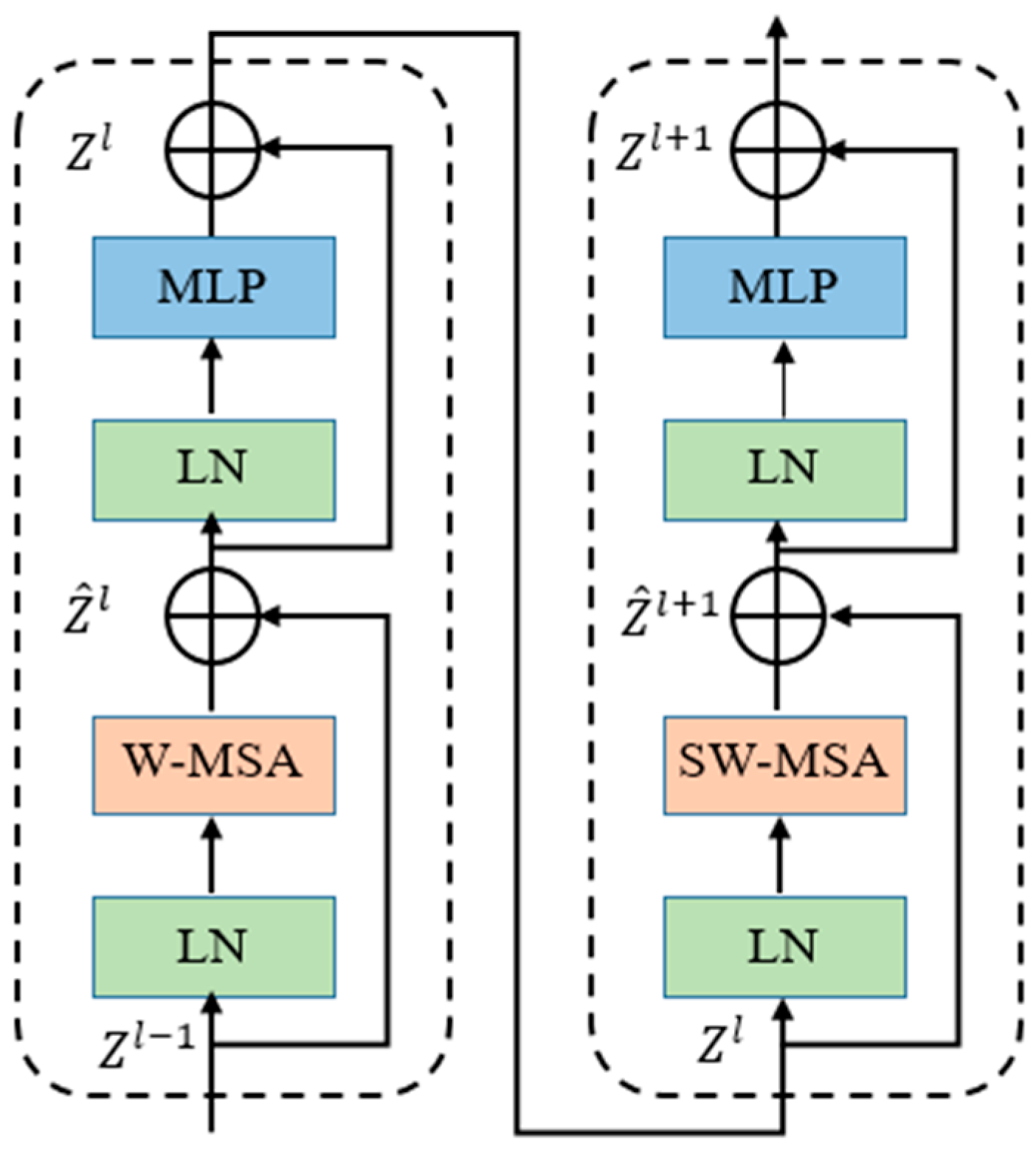
3.2. Swin Transformer

To overcome these limitations, the Microsoft Research Asia team proposed Swin Transformer (Swin) as an improvement over ViT. Swin introduces a hierarchical window mechanism that better captures local information and details in images through local window-level attention. Swin has achieved remarkable performance in image classification tasks and further advanced the development of transformer-based computer vision research. The structure of the Swin Transformer is illustrated in Figure 5.

Swin consists of four stages, and the specific process is as follows:

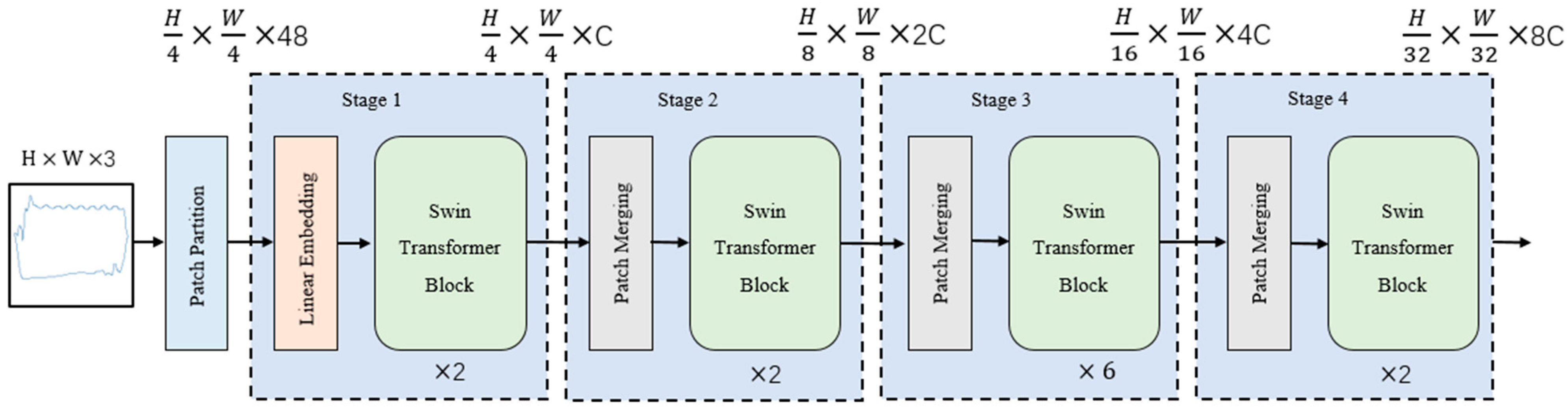
• Image Patch Division and Linear Embedding: The original image is divided into uniform image patches with dimensions of (H/4) × (W/4), where H and W represent the height and width of the input image, respectively. Each image patch’s feature dimension is then converted to C dimensions through linear embedding, where C corresponds to the number of channels in the Swin Transformer module.
• Image Patch Merging and Convolutional Dimension Reduction: Adjacent image patches are merged to form larger image patches. This reduces the number of image patches, and each merged image patch contains more local contextual information. The merged image patches undergo a convolutional network for dimension reduction, reducing the feature dimension to half of its original size. This helps to extract more abstract features.
• Repeat Stage 2: The process of image patch merging and convolutional dimension reduction in Stage 2 is repeated multiple times. With each repetition, the number of image patches is halved, and the feature dimension is also halved, while extracting higher-level feature representations.
• Swin Transformer Module: After Stage 3, the input is passed to the Swin Transformer module for computation. This module is based on the transformer architecture and processes the input using self-attention mechanisms and feed-forward neural network layers. It learns global contextual information and feature relationships to improve the quality of feature representation.

The Swin Transformer adopts a window-based multi-head self-attention module called “Windows Multi-Head Self-Attention” (W-MSA) in place of the traditional multi-head self-attention mechanism (MSA) used in the original transformer module. W-MSA is a modified version of self-attention specifically designed for attention calculation in the Swin Transformer. The computational complexities of MSA and W-MSA are as follows:

$${\Omega }_{MSA}=4hw{C}^2+2{\left(hw\right)}^{2}C$$

(5)

$${\Omega }_{W-MSA}=4hw{C}^2+2M^{2}hwC$$

(6)

where $C$ represents the depth of the image. $h$ and $w$ represent the height and width of the image. $M$ represents the size of the window.

Figure 6 illustrates two consecutive Swin Transformer modules. The input image features undergo layer normalization (LN) before being independently processed by the W-MSA module and the multi-layer perceptron (MLP). Additionally, each module is connected to the other through a residual connection, and another layer normalization layer follows this connection.

The computation process for feature propagation in the W-MSA module can be summarized as follows:

$${\hat{z}}^l=f_{W-MSA}\left[f_{LN}\left(z^{l-1}\right)\right]+z^{l-1}$$

(7)

$$z^l=f_{MLP}\left[f_{LN}\left({\widehat{z}}^l\right)\right]+{\widehat{z}}^l$$

(8)

where ${\widehat{z}}^l$ and $z^l$ refer to the output features of the W-MSA and MLP modules, respectively. $f_{W-MSA}$, $f_{MLP}$, and $f_{LN}$ represent the output functions of the W-MSA module, MLP module, and layer normalization, respectively.

Due to the non-overlapping nature of the cropped image patches in the W-MSA module, there is a lack of effective information interaction between the windows. To further enhance the model’s performance, the shift window multi-head self-attention (SW-MSA) module is introduced. Compared to W-MSA, SW-MSA allows the windows to move. The SW-MSA achieves this by cyclically shifting the image upwards and cyclically shifting half of the window size to the left. The areas of the image that fall outside the window are relocated to the bottom and right of the window. Afterwards, the windows are segmented using the W-MSA method, which leads to a distinct window partitioning approach compared to traditional W-MSA. The computation formula for SW-MSA is given as follows:

$${\widehat{z}}^{l+1}=f_{SW-MSA}\left[f_{LN}\left(z^l\right)\right]+z^l$$

(9)

$$z^{l+1}=f_{MLP}\left[f_{LN}\left({\widehat{z}}^{l+1}\right)\right]+{\widehat{z}}^{l+1}$$

(10)

where ${\hat{z}}^{l+1}$ and $z^{l+1}$ represent the output features of the $l$ + 1 SW-MSA and MLP blocks, respectively, and $f_{SW-MSA}$ represents the output function of the SW-MSA module.

4. Experimental Design and Results

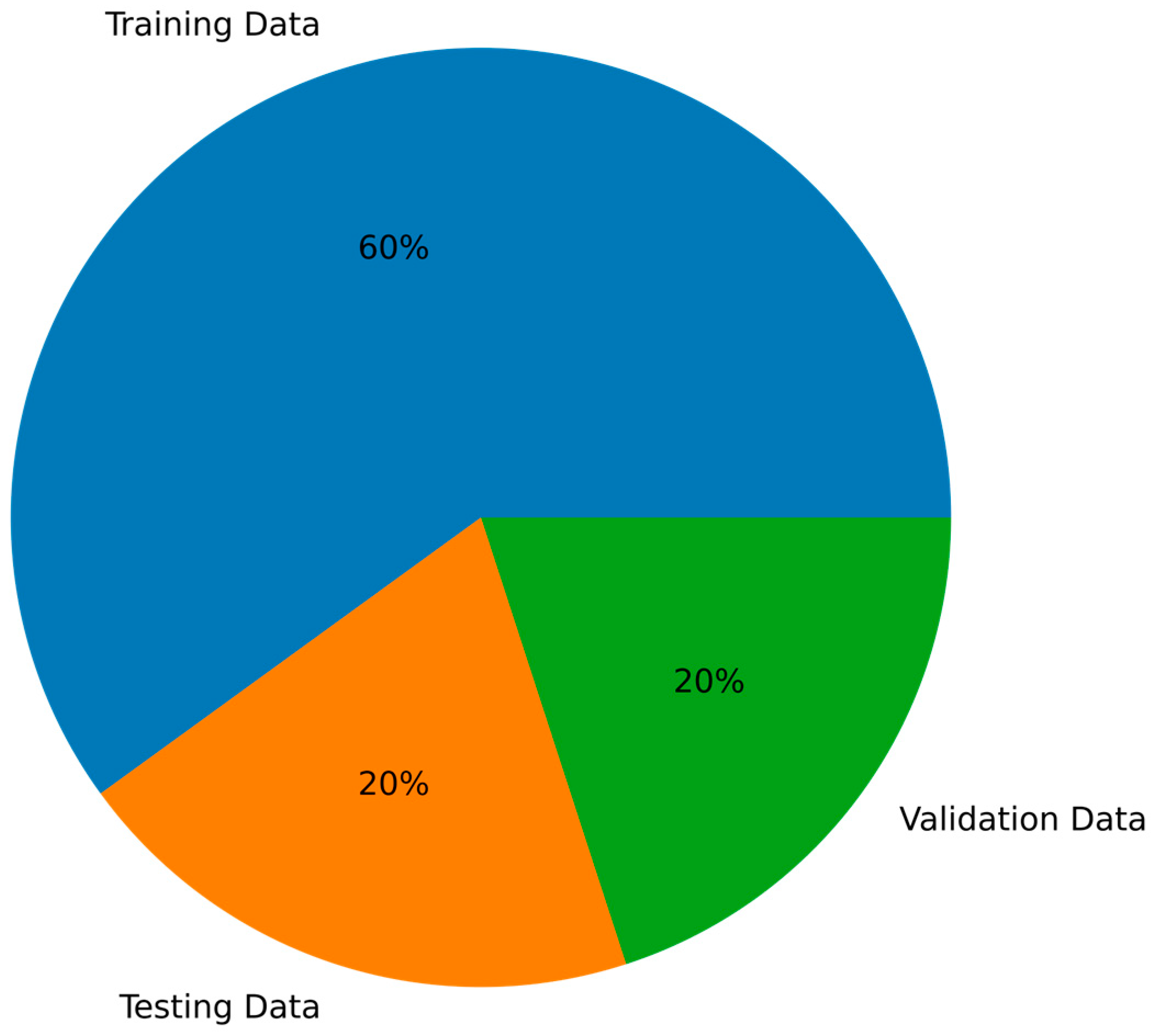
4.1. Dataset

The research utilized two primary datasets: the ImageNet-22k dataset and the oilfield dynagraph card dataset. The ImageNet-22k dataset is renowned in the machine learning domain for its broad applicability and has been extensively employed in previous studies [33]. Conversely, the oilfield dynagraph card dataset was gathered from real-time oilfield operations, lending practicality and authenticity to the research.

The ImageNet-22k dataset consists of 22,000 categories and an extended dataset with over 100 million image samples. Compared to ImageNet-1k, which has 1000 categories, ImageNet-22k covers a wider range of objects, scenes, and concepts. The image data are collected through web crawling, crowdsourced annotation, and filtering, encompassing various scenes, perspectives, and qualities. This dataset is primarily used for training and evaluating computer vision models, including tasks such as image classification, object detection, and image generation. With more categories and samples, ImageNet-22k presents a higher level of challenge for models, requiring better generalization to recognize and understand a broader range of objects and scenes.

The dynagraph card dataset is derived from real pumping units and contains dynagraph card curve data. The acquisition process of these data involves manual measurement and recording using instruments, which inevitably introduces some errors. These errors can be attributed to measurement inaccuracies of the instruments, sensor noise, environmental factors, and human factors. In actual oil pumping processes, there are various pumping conditions, but the main types include normal operation, fluid pound, gas influence, gas lock, delayed closing of the traveling valve, pump barrel slippage, and the combination of fluid pound and delayed closing of the traveling valve. Therefore, the original dynagraph card dataset was filtered, resulting in a total of 11,928 datasets, with 1704 data points per category. The splitting of a dataset into training, testing, and validation sets is implemented to effectively evaluate the model’s performance and enhance its generalization capabilities. The criterion for partitioning is randomly chosen to ensure that each subset is a representative sample of the data. Typically, the split ratios involve allocating a substantial portion of the data to the training set, a smaller proportion to the testing set, and including a validation set size that is often comparable to the testing set. In the article, the training set constitutes 60% of the data, while both the testing and validation sets each account for 20%. These datasets were divided into a training set (7000 data points, 1000 per category), a test set (2464 data points, 352 per category), and a validation set (2464 data points, 352 per category). Refer to Figure 7 for an illustration.

4.2. Experimental Process

In this paper, we conducted experiments in four stages: pre-training, training, testing, and validation. The experimental workflow is illustrated in Figure 8.

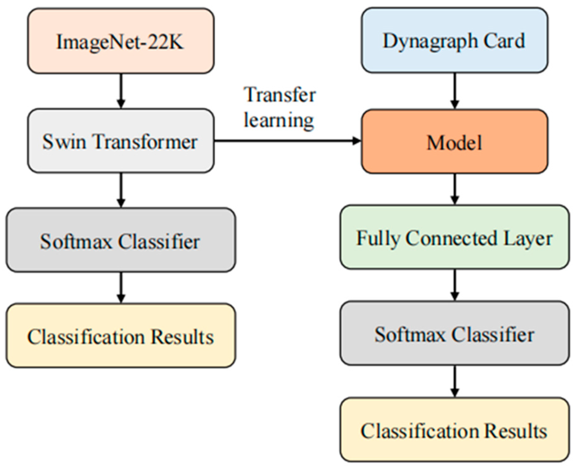
• Pre-Training Stage: First, we loaded a pre-trained Swin Transformer model as the feature extractor. This model consists of multiple layers of transformer structures that effectively handle image data. We used pre-trained weights obtained through self-supervised learning on the ImageNet-22k dataset, which provide high-level semantic feature representations [34]. Next, we added several fully connected layers to map the extracted features to the target classes. These additional layers were initialized with random weights and trained using backpropagation. During this process, we kept the pre-trained feature extractor fixed and only trained the additional layers. This allowed the model to adapt to our specific task and effectively train on limited labeled data [35].
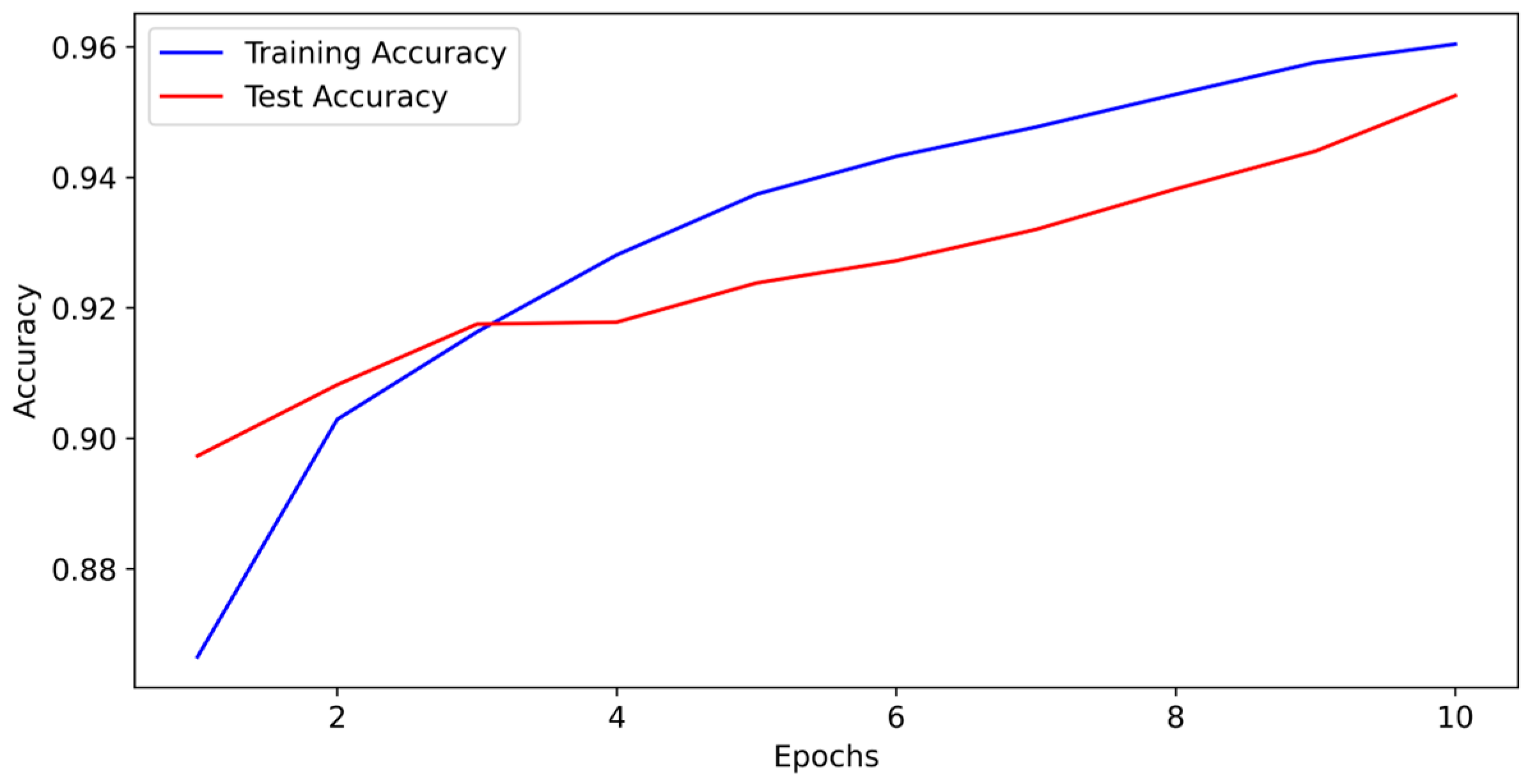
• Training Stage: During the training phase, we used the labeled training dataset of dynagraph cards to train the model. We employed the stochastic gradient descent optimization algorithm and utilized the cross-entropy loss function as the optimization objective for the model. The training dataset was divided into training and test sets, used for monitoring the training progress and model selection [36]. In each training batch, we randomly selected a batch of image samples from the training set and fed them into the model for forward and backward propagation. During the backward propagation process, the model updated its weight parameters based on the gradient information of the loss function. We evaluated the model using the test set, monitoring its accuracy and loss during the training process. We set a total of 10 training epochs, where each epoch corresponds to a complete traversal of the entire training dataset. Throughout the training process, we aimed for the model to learn effective feature representations and exhibit improved accuracy on the test set.
• Testing Stage: In the testing stage, we input the test set images into the model for inference, obtaining classification results and evaluating the model’s performance. The parameters used are consistent with those in the training stage.
• Validation Stage: In the validation stage, we input the validation set images into the model for evaluation, obtaining classification results and evaluating the model’s performance. The parameters used are consistent with those in the training stage.

4.3. Findings and Analysis from the Experiments

In this paper, we will evaluate the model using the test set based on four evaluation metrics: accuracy, ROC curve, confusion matrix, and P-R curve.

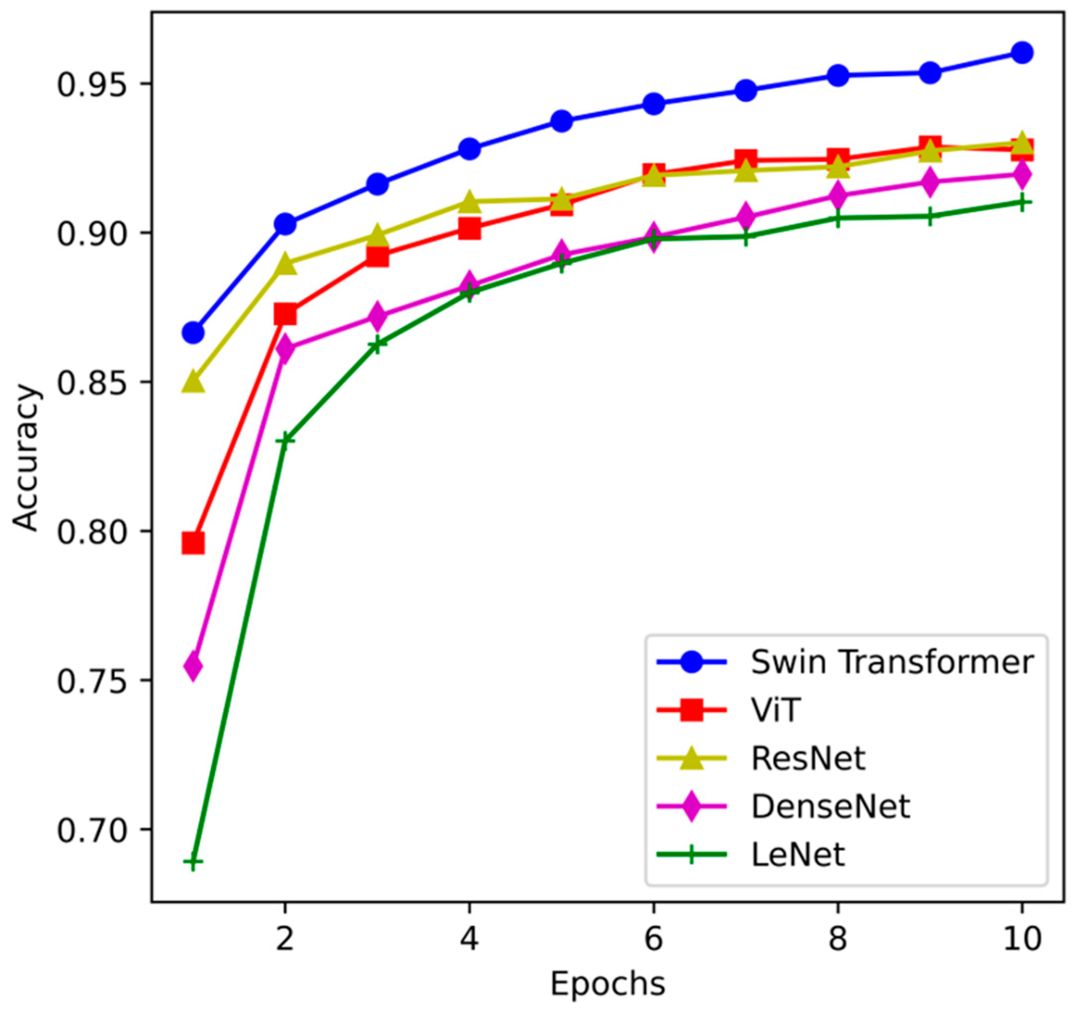
4.3.1. Accuracy

Throughout the model’s training and testing phases, we conducted 10 iterations and generated an accuracy curve based on the achieved accuracy in each iteration, as depicted in Figure 9. The model demonstrated outstanding training performance, with a final training accuracy of 96.04%.

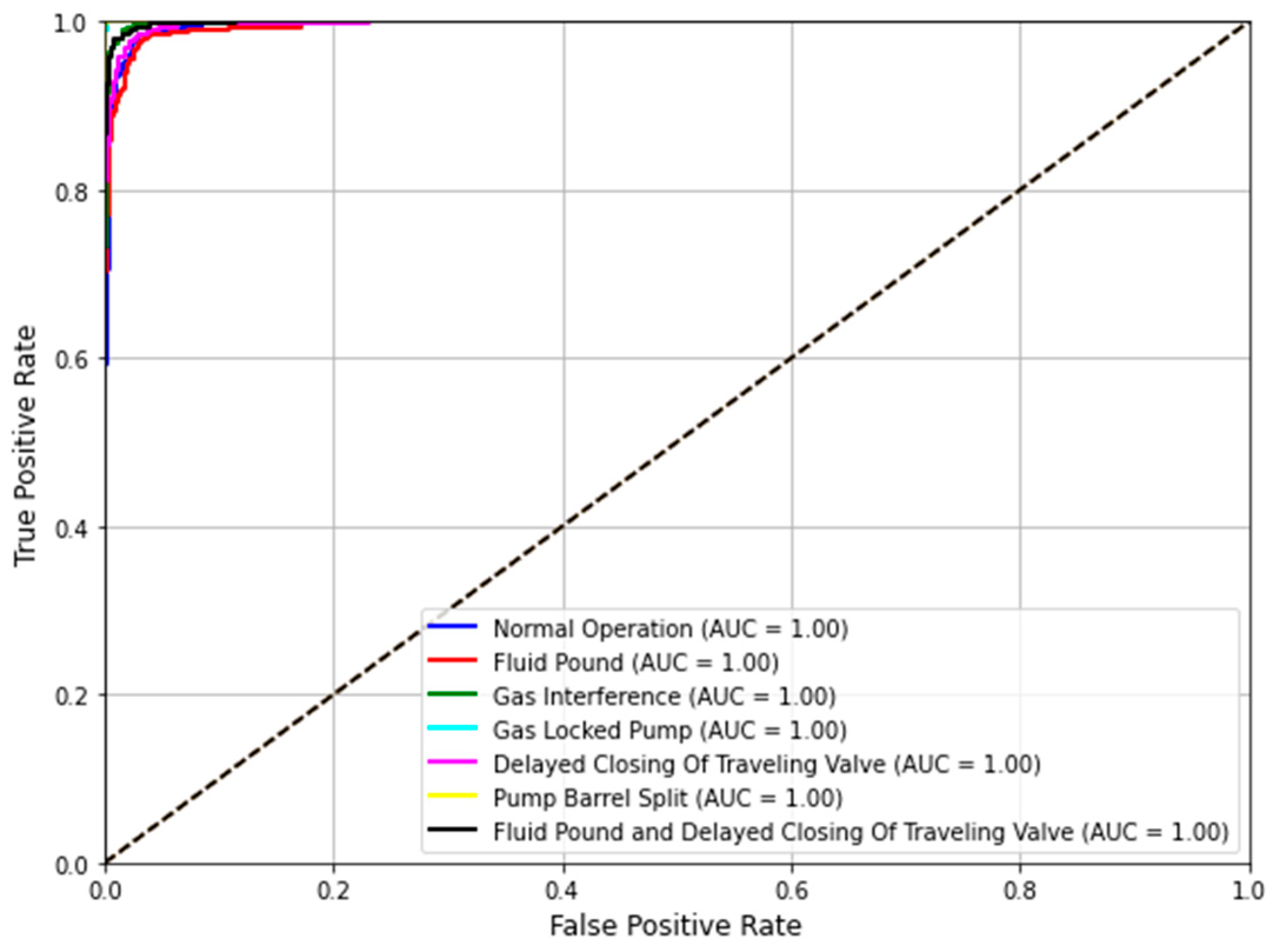
4.3.2. ROC Curve

The receiver operating characteristic (ROC) curve is a widely employed tool in machine learning and statistics for assessing the performance of classification models. It is constructed by plotting the true positive rate (TPR) on the y-axis against the false positive rate (FPR) on the x-axis [37].

To generate the ROC curve, the classification model is applied to predict the samples within the test set, obtaining either predicted probabilities or decision scores for each sample. These scores are then utilized to arrange the samples in descending order. Starting from the lowest threshold, all samples are initially labeled as the negative class, and the TPR and FPR are calculated accordingly.

$$TPR=\frac{TP}{TP+FN}$$

(11)

$$FPR=\frac{FP}{FP+TN}$$

(12)

In this context, TP refers to the count of true positives, which represents the instances correctly predicted as the positive class and which are actually positive. FN corresponds to the count of false negatives, indicating the instances that are incorrectly predicted as the negative class but are actually positive. FP represents the count of false positives, signifying the instances erroneously predicted as the positive class but which are actually negative. Lastly, TN denotes the count of true negatives, which indicates the instances correctly predicted as the negative class and which are actually negative. By gradually decreasing the threshold, the steps are repeated, and the TPR and FPR are calculated for different thresholds. All computed TPR and FPR values are plotted to form the ROC curve.

When the model can perfectly distinguish between positive and negative classes, the curve will pass through the points (0,0) and (1,1), forming a straight line with a unit slope. When the model cannot distinguish between positive and negative classes, the ROC curve will approach the diagonal line. By observing the ROC curve, we can choose an appropriate threshold based on the specific requirements to balance the true positive rate and false positive rate. In general, the larger the area under the curve (AUC), the better the model performance. The Area Under the Curve (AUC) varies between 0.5 and 1, with 0.5 representing a model’s performance equivalent to random guessing, and 1 indicating flawless classification by the model.

We have generated the ROC curves for each class, as depicted in Figure 10. The graphs clearly demonstrate that the classification performance for each class is exceptional, indicating an outstanding model performance.

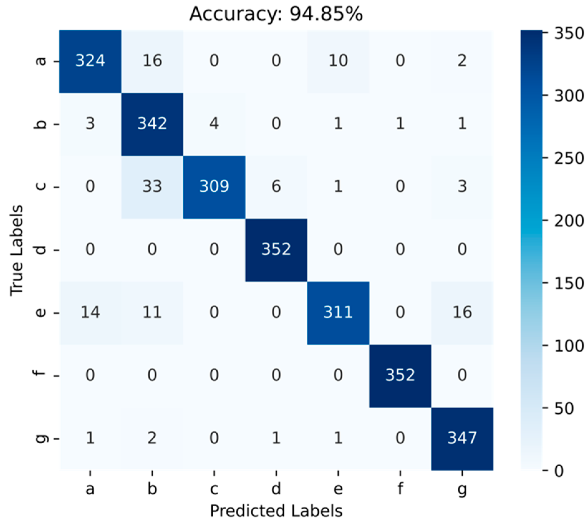
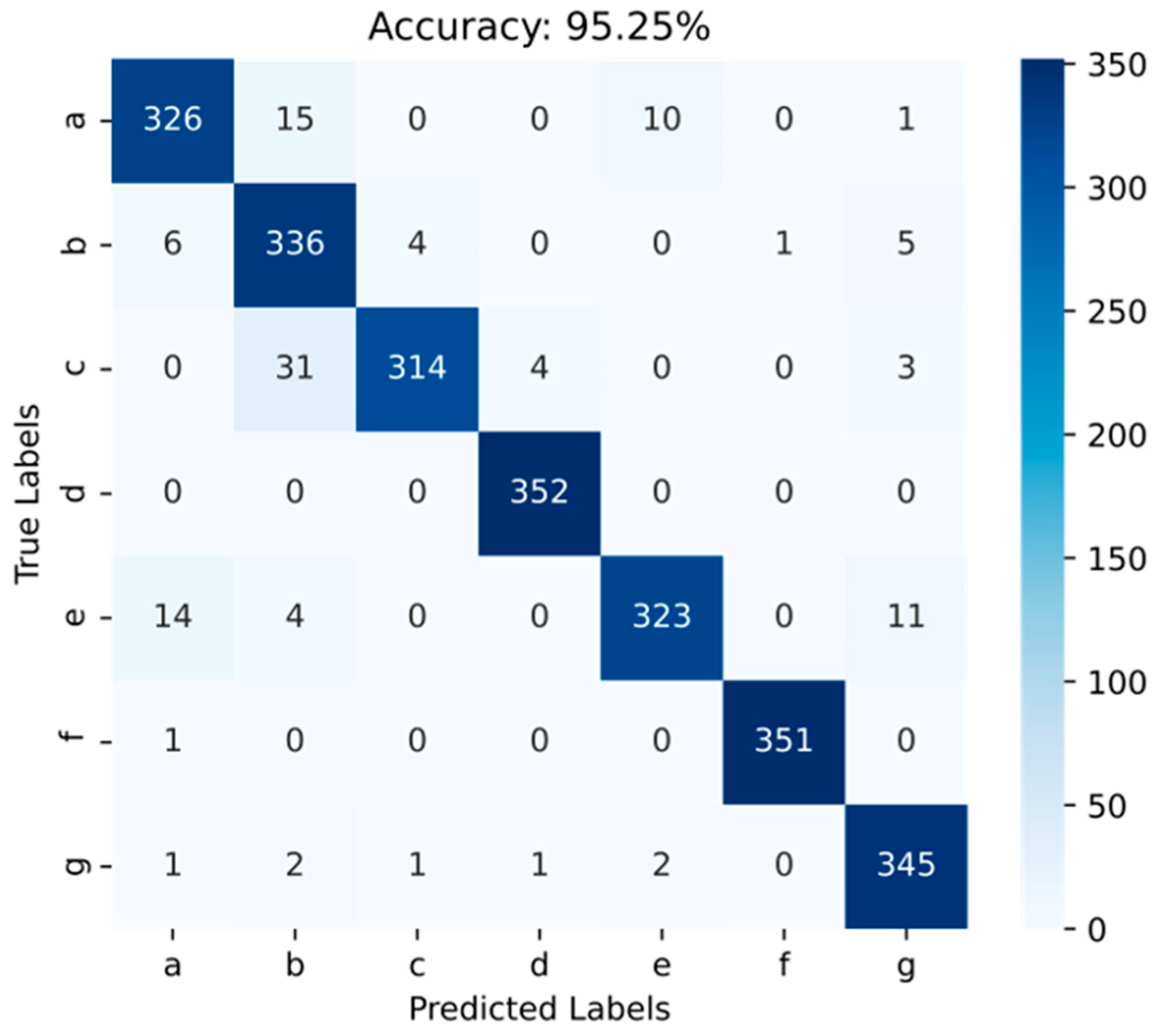
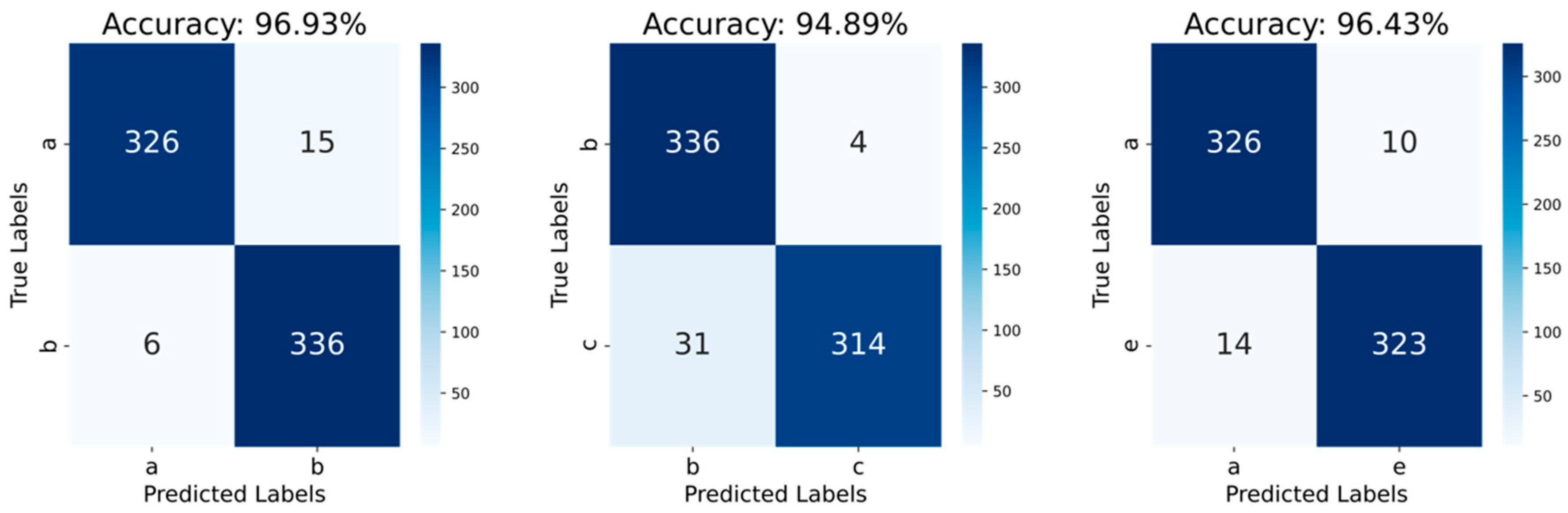
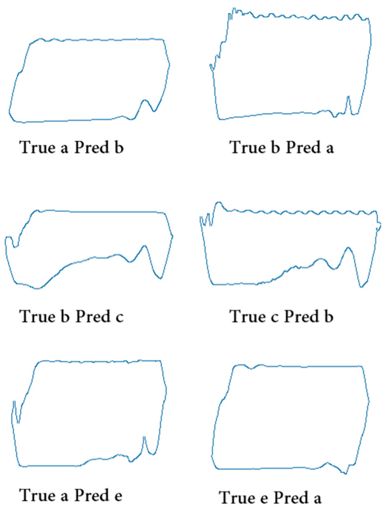
4.3.3. Confusion Matrix

The confusion matrix is a tabular representation commonly employed to assess the performance of a classification model, illustrating the correlation between the model’s predictions and the actual outcomes on a test dataset [38]. It serves as a valuable tool in classification problems, providing a detailed evaluation of the model’s behavior and performance.

The confusion matrix is presented as a two-dimensional table, with rows indicating the actual classes and columns representing the predicted classes made by the model.

Table 1. Confusion matrix.

		Predicted Results
		Positive Example	Negative Example
Real results	Positive example	TP	FN
	Negative example	FP	TN

illustrates an exemplar confusion matrix.

In the confusion matrix, TP represents the correct prediction of positive samples as positive, indicating that the model correctly identifies the true positives. This means that the model successfully classifies positive instances as positive. TN represents the correct prediction of negative samples as negative, indicating that the model correctly identifies the true negatives. This means that the model successfully classifies negative instances as negative. FP represents the model’s incorrect prediction of negative samples as positive, also known as Type I Error, indicating that the model incorrectly identifies actual negatives as positives. FN represents the model’s incorrect prediction of positive samples as negative, also known as Type II Error, indicating that the model incorrectly identifies actual positives as negatives.

Figure 11 displays the confusion matrix for the test dataset, providing a clear depiction of the classification accuracy performance for each class. The matrix reveals that the likelihood of misclassification between classes is minimal, indicating a model with excellent classification capabilities.

It can be observed that there are some incorrect predictions in the classes of Normal Operation, Fluid Pound, Gas Interference, and Delayed Closing of Traveling Valve. We have separately plotted the confusion matrices between these classes, as shown in Figure 12.

From Figure 12, the model demonstrates a classification accuracy exceeding 0.94 for the classes of Normal Operation, Fluid Pound, Gas Interference, and Delayed Closing of Traveling Valve. This indicates that the Swin Transformer model is capable of accurately distinguishing similar waveform patterns under different working conditions, and it exhibits excellent performance.

When we selected some dynagraph cards and compared them, as shown in Figure 13, we found that there were some incorrect predictions. Particularly notable is that in the classes of Normal Operation, Fluid Pound, Gas Interference, and Delayed Closing of Traveling Valve, the waveform patterns of the dynagraph cards may exhibit similarities, especially under certain specific operating conditions. This makes it challenging for the model to accurately differentiate between different classes in these similar waveforms.

The dynagraph card data may contain some noise, which could interfere with the model’s learning process. This noise can lead to erroneous biases in the model’s predictions for similar waveforms, consequently affecting its classification performance.

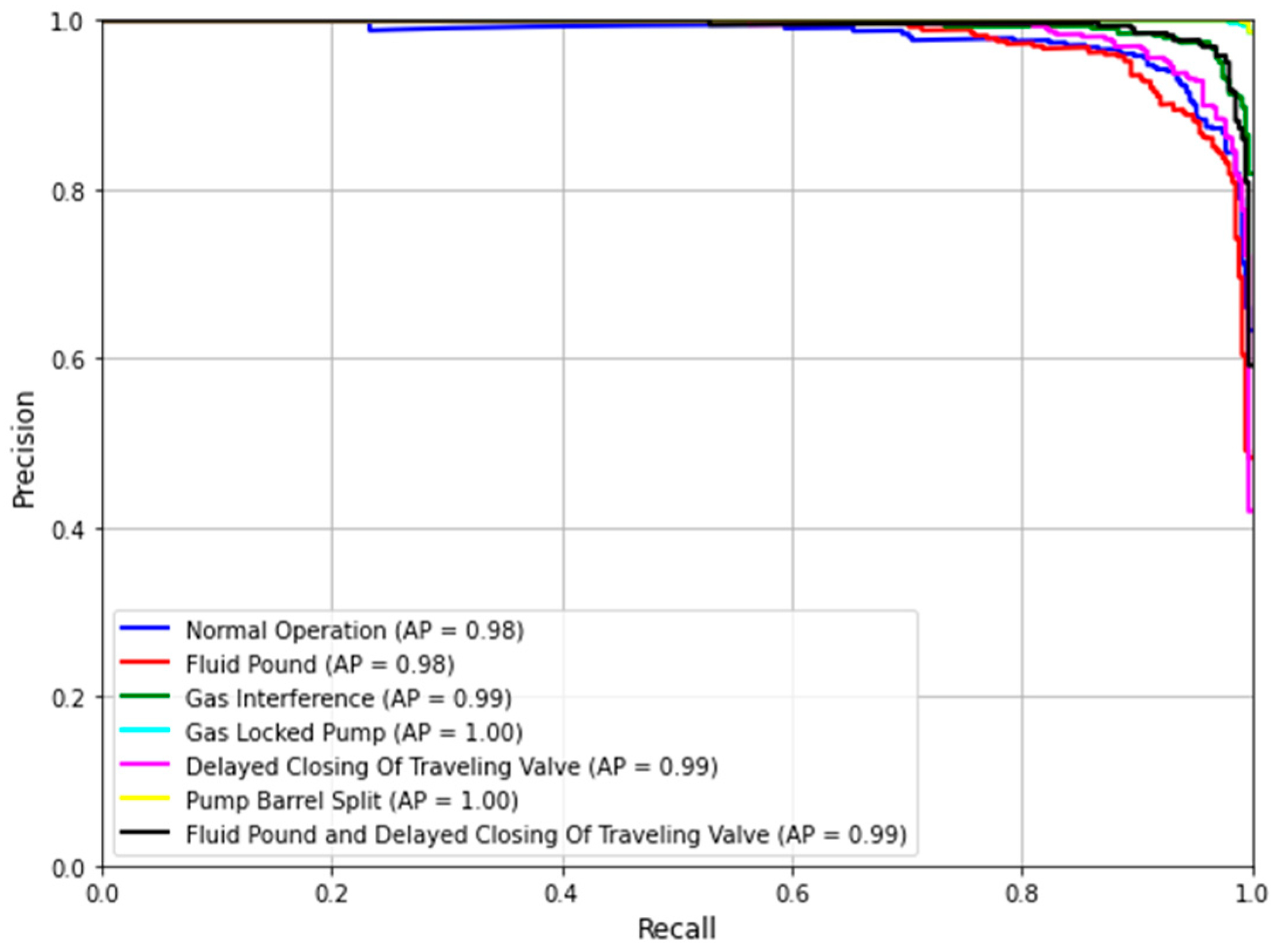
4.3.4. P-R Curve

The precision–recall (P-R) curve is a widely adopted approach for evaluating the performance of classification models, particularly when dealing with imbalanced datasets [39]. PR represents “Precision” and “Recall”, two essential metrics in classification evaluation. Precision is the proportion of true positive samples among the samples predicted as positive by the classifier. In other words, it measures the accuracy of positive predictions made by the model. Recall, on the other hand, is the proportion of true positive samples among all the actual positive samples. It gauges the model’s ability to capture all positive instances correctly, without missing any. The P-R curve offers valuable insights into how well a classification model performs, especially in scenarios where class distribution is imbalanced. The calculation formulas are as follows:

$$Precision=\frac{TP}{TP+FP}$$

(13)

$$Recall=\frac{FP}{FP+TN}$$

(14)

In this context, TP represents the count of true positives, which signifies the instances correctly predicted as the positive class. FP refers to the count of false positives, representing the instances incorrectly predicted as the positive class. FN represents the count of false negatives, indicating the instances that were incorrectly predicted as the negative class. Firstly, the classification model is used to predict the samples in the test set, and the probabilities or confidences of each sample are calculated based on the predictions. Secondly, the samples in the test set are sorted based on their probabilities or confidences. Starting from the sample with the highest probability or confidence, each sample is added to the positive set one by one, and the precision and recall are calculated at each step. Finally, the precision and recall values are plotted on a coordinate system to form the PR curve.

Average precision (AP) is a performance metric utilized to assess information retrieval systems, object detection, classification models, and various other tasks. It takes values between 0 and 1, where higher values correspond to superior model performance. A higher AP means that the model can maintain a higher precision at different recall levels.

$$AP=\sum _n(R_n-R_{n-1})P_n$$

(15)

We have generated the PR curves for each class, as illustrated in Figure 14. Observing the graph, it becomes evident that the curves for each class exhibit a well-balanced nature, with average precision values exceeding 0.98. This observation indicates that the model performs exceptionally well in terms of detecting incorrect classes and overall model performance.

4.4. Comparative Experimental Analysis

4.4.1. Model Performance Comparison

To establish the superiority of our proposed model, we conducted a comparative analysis with common image classification models, namely ResNet50 [40], DenseNet121 [41], LeNet [42], and ViT models. All models were trained and tested on the same schematic dataset used in this study, using identical model parameters and pre-trained weights obtained through transfer learning.

The accuracy curves during the training process are illustrated in Figure 15. Upon completing the final iterations, the training accuracies for each model were as follows: Swin Transformer = 96.04%, ViT = 92.78%, LeNet = 91.03%, DenseNet121 = 91.96%, and ResNet50 = 93.02%. Remarkably, the Swin Transformer model exhibited significantly higher classification accuracy when compared to all other models.

The performance metrics of all models are compared in

Table 2. Comparison of results of the test sets for each model.

	Model	Accuracy	F1 Score	Precision	Recall	ROC AUC	K
Transformer	Swin-T	0.952	0.952	0.954	0.952	0.972	0.923
	ViT	0.944	0.944	0.945	0.944	0.957	0.901
CNN	ResNet	0.912	0.906	0.918	0.915	0.937	0.872
	DenseNet	0.897	0.896	0.902	0.897	0.940	0.885
	LeNet	0.890	0.887	0.898	0.884	0.918	0.862

. It can be observed that the transformer models outperform the CNN models overall. This can be attributed to the following reasons: The transformer model utilizes self-attention mechanisms to capture global information in the schematic diagrams and model the relationships between different parts. This enables the model to better understand the importance and interactions of different features in the schematic diagrams, thereby improving classification accuracy. The self-attention mechanism in the transformer model allows the output at each position to be influenced by other positions, enabling parameter sharing. This characteristic of parameter sharing allows the transformer model to handle schematic diagram data more efficiently, reducing the number of model parameters and computational complexity. Transformer models are typically initialized with parameters from pre-trained models on large-scale datasets, providing better initial representation capabilities. This allows the transformer model to converge and adapt to the schematic diagram classification task more quickly, resulting in improved model performance.

The proposed Swin Transformer model in this paper performs better in addressing the recognition problem among similar but distinct categories of schematic diagrams. By leveraging the influence of self-attention values on image patches, the Swin Transformer model can focus more on informative features that contribute to classification and avoid negative effects caused by the similarity between schematic diagrams. As a result, the Swin Transformer model achieves the best performance in the task of schematic diagram classification.

4.4.2. Model Computational Comparison

When evaluating deep learning models, two important metrics to consider are the number of parameters (Param) and the computational complexity (FLOPs) [43]. Different models exhibit distinct differences in terms of parameter count and computational complexity. Generally, a higher parameter count indicates a higher modeling capacity, but it also increases the computational burden. Similarly, a higher computational complexity requires more computing resources for training and inference. Therefore, when selecting a model, it is crucial to balance the number of parameters and computational complexity to meet the specific requirements of the task while considering the limitations of computing resources [44]. As shown in

Table 3. Comparison of results for each model.

	Model	Param (M)	FLOPs (G)
Transformer	Swin-T	0.38	8.7
	ViT	0.25	743.0
CNN	ResNet	24.5	3.9
	DenseNet	6.69	2.91
	LeNet	0.06	0.005

, we can compare the computational aspects of the given models.

As shown in the table above, among the transformer-based models, the Swin Transformer model has a parameter count of 0.38 M and a computational complexity of 8.7 G FLOPs. On the other hand, the ViT model has a lower parameter count of 0.25 M but a significantly higher computational complexity of 743.0 G FLOPs. This indicates that the ViT model is computationally more expensive and requires larger computational resources compared to the Swin Transformer model.

Among the CNN-based models, the ResNet model has a larger parameter count of 24.51 M but a relatively lower computational complexity of 3.9 G FLOPs. The DenseNet model has a parameter count of 6.69 M, slightly lower than ResNet, and a computational complexity of 2.91 G FLOPs. LeNet, being a very simple model, has the smallest parameter count and computational complexity, with only 0.06 M parameters and 0.005 G FLOPs.

The Swin Transformer has a higher parameter count compared to ViT. This is because the Swin Transformer employs a block-based strategy, dividing the image into smaller blocks and then performing self-attention operations on these blocks, reducing the computational complexity of the model. In contrast, ViT uses a global self-attention mechanism, requiring self-attention operations across the entire image, resulting in higher computational complexity. Although the LeNet model is relatively simple, oilfield dynagraph data typically contain rich information and complex patterns, necessitating a more powerful model to accurately capture these features for effective fault diagnosis. The Swin Transformer offers superior modeling capabilities and performance, contributing to improved diagnostic accuracy, especially when dealing with large-scale dynagraph cards, whereas the simplicity of the LeNet model may not fully leverage these data to achieve the same level of performance. Therefore, for complex tasks like oilfield dynagraph fault diagnosis, the Swin Transformer is more conducive to enhancing diagnostic efficiency and accuracy.

4.5. Model Validation

To assess the applicability of the Swin Transformer model in real oilfield scenarios, we can employ the validation set to evaluate the model’s performance on oilfield instances. Firstly, we preprocess the well test data in the same manner as before and then employ the trained model to make predictions on the data. By comparing the model’s predicted results with the ground truth labels, we generate a confusion matrix to illustrate their relationship, as shown in Figure 16.

Based on the graph, it is evident that the Swin Transformer model attains a prediction accuracy of 94.85% on the validation set. This outstanding performance showcases the model’s robust generalization capability and its excellent suitability for real oilfield field development applications.

5. Conclusions

This research introduces a dynagraph card diagnosis approach using the Swin Transformer, demonstrating its superior performance compared to traditional convolutional neural network methods and ViT methods in dynagraph card condition diagnosis. The experimental results and analysis have led to the following conclusions:

• To address the classification problem of dynagraph cards in the rod pumping system, we have developed a neural network model based on attention mechanisms to achieve the effective identification and classification of Normal Operation, Fluid Pound, Gas Interference, Gas Locked Pump, Delayed Closing of Traveling Valve, Pump Barrel Split, and Fluid Pound and Delayed Closing of Traveling Valve. Compared to previous methods, this approach enables the more efficient and accurate automatic identification of dynagraph cards.
• By utilizing the Swin Transformer model and transfer learning, we introduce a hierarchical window mechanism through the Swin Transformer, which captures local information and details in images more effectively through local window-level attention mechanisms, thus improving the accuracy of condition diagnosis. Transfer learning allows our model to benefit from the pre-trained Swin Transformer model parameters, improving training efficiency and saving time. However, the model to some extent relies on large-scale datasets to achieve better performance.
• Our method demonstrates high accuracy in pumping unit condition diagnosis and holds significant research value for intelligent oilfield development.

Although the Swin Transformer model has achieved remarkable results in dynagraph card diagnostics through transfer learning, its success relies on the support of manually labeled dynagraph card data. This process involves investments in both human resources and finances. In future investigations, we will persist in exploring alternative methodologies to further improve the accuracy of condition diagnosis. Moreover, our future endeavors involve integrating multimodal techniques with pumping system analysis, aiming to accomplish real-time condition diagnosis and the intelligent analysis of oilfield well sites.

References

- Parimontonsakul, M.; Lotongkum, S.; Mularlee, K. A Machine Learning Based Approach to Automate Stratigraphic Correlation through Marker Determination. Improv. Oil Gas Recovery 2023, 7, 1. [Google Scholar]
- Tian, J.; Gao, M.; Li, K.; Zhou, H. Fault Detection of Oil Pump Based on Classify Support Vector Machine. In Proceedings of the 2007 IEEE International Conference on Control and Automation, Guangzhou, China, 30 May–1 June 2007; pp. 549–553. [Google Scholar]
- Li, K.; Gao, X.; Tian, Z.; Qiu, Z. Using the Curve Moment and the PSO-SVM Method to Diagnose Downhole Conditions of a Sucker Rod Pumping Unit. Pet. Sci. 2013, 10, 73–80. [Google Scholar] [CrossRef]
- He, Y.; Liu, Y.; Shao, S.; Zhao, X.; Liu, G.; Kong, X.; Liu, L. Application of CNN-LSTM in Gradual Changing Fault Diagnosis of Rod Pumping System. Math. Probl. Eng. 2019, 2019, 4203821. [Google Scholar] [CrossRef]
- Zhou, X.; Zhao, C.; Liu, X. Application of Cnn Deep Learning to Well Pump Troubleshooting via Power Cards. In Proceedings of the Abu Dhabi International Petroleum Exhibition and Conference, Abu Dhabi, United Arab Emirates, 11–14 November 2019; p. D031S090R004. [Google Scholar]
- Cheng, H.; Yu, H.; Zeng, P.; Osipov, E.; Li, S.; Vyatkin, V. Automatic Recognition of Sucker-Rod Pumping System Working Conditions Using Dynamometer Cards with Transfer Learning and Svm. Sensors 2020, 20, 5659. [Google Scholar] [CrossRef]
- Wibawa, R.; Rosyadi, R.; Nancy, M.; Irfani Hasya Fulki, R. Unlocking the Potential of Unlabeled Data in Building Deep Learning Model for Dynamometer Cards Classification by Using Self-Supervised Learning. In Proceedings of the International Petroleum Technology Conference, Bangkok, Thailand, 1–3 March 2023. [Google Scholar] [CrossRef]
- Zhang, L.; Wu, J.; Zhang, K.; Wang, Z.; Yan, X.; Liu, P.; Wang, Q.; Fan, L.; Yao, J.; Yang, Y. Diagnosis of Pumping Machine Working Conditions Based on Transfer Learning and ViT Model. Geoenergy Sci. Eng. 2023, 226, 211729. [Google Scholar] [CrossRef]
- Dosovitskiy, A.; Beyer, L.; Kolesnikov, A.; Weissenborn, D.; Zhai, X.; Unterthiner, T.; Dehghani, M.; Minderer, M.; Heigold, G.; Gelly, S. An Image Is Worth 16x16 Words: Transformers for Image Recognition at Scale. arXiv 2020, arXiv:2010.11929. [Google Scholar]
- Liu, Z.; Lin, Y.; Cao, Y.; Hu, H.; Wei, Y.; Zhang, Z.; Lin, S.; Guo, B. Swin Transformer: Hierarchical Vision Transformer Using Shifted Windows. In Proceedings of the IEEE/CVF International Conference on Computer Vision, Montreal, BC, Canada, 11–17 October 2021; pp. 10012–10022. [Google Scholar]
- Solodkiy, E.M.; Kazantsev, V.P.; Dadenkov, D.A. Improving the Energy Efficiency of the Sucker-Rod Pump via Its Optimal Counterbalancing. In Proceedings of the 2019 International Russian Automation Conference (RusAutoCon), Sochi, Russia, 8–14 September 2019; pp. 1–5. [Google Scholar]
- Xing, M.; Dong, S. A New Simulation Model for a Beam-Pumping System Applied in Energy Saving and Resource-Consumption Reduction. SPE Prod. Oper. 2015, 30, 130–140. [Google Scholar] [CrossRef]
- Ruset, I.C.; Ketel, S.; Hersman, F.W. Optical Pumping System Design for Large Production of Hyperpolarized Xe 129. Phys. Rev. Lett. 2006, 96, 053002. [Google Scholar] [CrossRef] [PubMed]
- Gibbs, S.G. A General Method for Predicting Rod Pumping System Performance. In Proceedings of the SPE Annual Technical Conference and Exhibition? Denver, CO, USA, 2 October 1977; p. SPE-6850-MS. [Google Scholar]
- Xu, P.; Xu, S.; Yin, H. Application of Self-Organizing Competitive Neural Network in Fault Diagnosis of Suck Rod Pumping System. J. Pet. Sci. Eng. 2007, 58, 43–48. [Google Scholar] [CrossRef]
- Gibbs, S.G. Predicting the Behavior of Sucker-Rod Pumping Systems. J. Pet. Technol. 1963, 15, 769–778. [Google Scholar] [CrossRef]
- Feng, Z.-M.; Guo, C.; Zhang, D.; Cui, W.; Tan, C.; Xu, X.; Zhang, Y. Variable Speed Drive Optimization Model and Analysis of Comprehensive Performance of Beam Pumping Unit. J. Pet. Sci. Eng. 2020, 191, 107155. [Google Scholar] [CrossRef]
- Boguslawski, B.; Boujonnier, M.; Bissuel-Beauvais, L.; Saghir, F.; Sharma, R.D. IIoT Edge Analytics: Deploying Machine Learning at the Wellhead to Identify Rod Pump Failure. In Proceedings of the SPE Middle East Artificial Lift Conference and Exhibition, Manama, Bahrain, 28–29 November 2018; p. D021S004R001. [Google Scholar]
- Yavuz, F.; Lea, J.F.; Garg, D.; Oetama, T.; Cox, J.; Nickens, H. Wave Equation Simulation of Fluid Pound and Gas Interference. In Proceedings of the SPE Oklahoma City Oil and Gas Symposium/Production and Operations Symposium, Oklahoma City, OK, USA, 16–19 April 2005; p. SPE-94326-MS. [Google Scholar]
- Allison, A.P.; Leal, C.F.; Boland, M.R. Solving Gas Interference Issues with Sucker Rod Pumps in the Permian Basin. In Proceedings of the SPE Artificial Lift Conference and Exhibition-Americas, The Woodlands, TX, USA, 28–30 August 2018. [Google Scholar] [CrossRef]
- Brauers, H.; Braunger, I.; Jewell, J. Liquefied Natural Gas Expansion Plans in Germany: The Risk of Gas Lock-in under Energy Transitions. Energy Res. Soc. Sci. 2021, 76, 102059. [Google Scholar] [CrossRef]
- Juch, A.H.; Watson, R.J. New Concepts in Sucker-Rod Pump Design. J. Pet. Technol. 1969, 21, 342–354. [Google Scholar] [CrossRef]
- Nickens, H.; Lea, J.F.; Cox, J.C.; Bhagavatula, R.; Garg, D. Downhole Beam Pump Operation: Slippage and Buckling Forces Transmitted to the Rod String. J. Can. Pet. Technol. 2005, 44, 5. [Google Scholar] [CrossRef]
- Chua, L.O.; Roska, T. The CNN Paradigm. IEEE Trans. Circuits Syst. I Fundam. Theory Appl. 1993, 40, 147–156. [Google Scholar] [CrossRef]
- Kuo, C.-C.J. Understanding Convolutional Neural Networks with a Mathematical Model. J. Vis. Commun. Image Represent. 2016, 41, 406–413. [Google Scholar] [CrossRef]
- Strubell, E.; Ganesh, A.; McCallum, A. Energy and Policy Considerations for Deep Learning in NLP. arXiv 2019, arXiv:1906.02243. [Google Scholar]
- Zhang, Q.; Zhu, S.-C. Visual Interpretability for Deep Learning: A Survey. Front. Inf. Technol. Electron. Eng. 2018, 19, 27–39. [Google Scholar] [CrossRef]
- Shaw, P.; Uszkoreit, J.; Vaswani, A. Self-Attention with Relative Position Representations. arXiv 2018, arXiv:1803.02155. [Google Scholar]
- Rawat, W.; Wang, Z. Deep Convolutional Neural Networks for Image Classification: A Comprehensive Review. Neural Comput. 2017, 29, 2352–2449. [Google Scholar] [CrossRef]
- Abbasi, S.F.; Ahmad, J.; Tahir, A.; Awais, M.; Chen, C.; Irfan, M.; Siddiqa, H.A.; Waqas, A.B.; Long, X.; Yin, B.; et al. EEG-based neonatal sleep-wake classification using multilayer perceptron neural network. IEEE Access 2020, 8, 183025–183034. [Google Scholar] [CrossRef]
- Han, K.; Wang, Y.; Chen, H.; Chen, X.; Guo, J.; Liu, Z.; Tang, Y.; Xiao, A.; Xu, C.; Xu, Y. A Survey on Vision Transformer. IEEE Trans. Pattern Anal. Mach. Intell. 2022, 45, 87–110. [Google Scholar] [CrossRef] [PubMed]
- Hatamizadeh, A.; Yin, H.; Heinrich, G.; Kautz, J.; Molchanov, P. Global Context Vision Transformers. In Proceedings of the International Conference on Machine Learning, Honolulu, HI, USA, 23–29 July 2023; pp. 12633–12646. [Google Scholar]
- Russakovsky, O.; Deng, J.; Su, H.; Krause, J.; Satheesh, S.; Ma, S.; Huang, Z.; Karpathy, A.; Khosla, A.; Bernstein, M. Imagenet Large Scale Visual Recognition Challenge. Int. J. Comput. Vis. 2015, 115, 211–252. [Google Scholar] [CrossRef]
- Weiss, K.; Khoshgoftaar, T.M.; Wang, D. A Survey of Transfer Learning. J. Big Data 2016, 3, 9. [Google Scholar] [CrossRef]
- Zhuang, F.; Qi, Z.; Duan, K.; Xi, D.; Zhu, Y.; Zhu, H.; Xiong, H.; He, Q. A Comprehensive Survey on Transfer Learning. Proc. IEEE 2020, 109, 43–76. [Google Scholar] [CrossRef]
- Ho, Y.; Wookey, S. The Real-World-Weight Cross-Entropy Loss Function: Modeling the Costs of Mislabeling. IEEE Access 2019, 8, 4806–4813. [Google Scholar] [CrossRef]
- Bradley, A.P. The Use of the Area under the ROC Curve in the Evaluation of Machine Learning Algorithms. Pattern Recognit. 1997, 30, 1145–1159. [Google Scholar] [CrossRef]
- Rahman, M.M.; Davis, D.N. Addressing the Class Imbalance Problem in Medical Datasets. Int. J. Mach. Learn. Comput. 2013, 3, 224. [Google Scholar] [CrossRef]
- Davis, J.; Goadrich, M. The Relationship between Precision-Recall and ROC Curves. In Proceedings of the 23rd International Conference on Machine Learning, Pittsburgh, PA, USA, 25–29 June 2006; pp. 233–240. [Google Scholar] [CrossRef]
- Targ, S.; Almeida, D.; Lyman, K. Resnet in Resnet: Generalizing Residual Architectures. arXiv 2016, arXiv:1603.08029. [Google Scholar]
- Iandola, F.; Moskewicz, M.; Karayev, S.; Girshick, R.; Darrell, T.; Keutzer, K. Densenet: Implementing Efficient Convnet Descriptor Pyramids. arXiv 2014, arXiv:1404.1869. [Google Scholar]
- Islam, M.R.; Matin, A. Detection of COVID 19 from CT Image by the Novel LeNet-5 CNN Architecture. In Proceedings of the 23rd International Conference on Computer and Information Technology (ICCIT), Dhaka, Bangladesh, 19–21 December 2020; pp. 1–5. [Google Scholar]
- Markovic, D.; Nikolic, B.; Brodersen, R. Analysis and Design of Low-Energy Flip-Flops. In Proceedings of the International Symposium on Low Power Electronics and Design, Huntington Beach, CA, USA, 6–7 August 2001; pp. 52–55. [Google Scholar] [CrossRef]
- Zhan, Z.-H.; Liu, X.-F.; Gong, Y.-J.; Zhang, J.; Chung, H.S.-H.; Li, Y. Cloud Computing Resource Scheduling and a Survey of Its Evolutionary Approaches. ACM Comput. Surv. (CSUR) 2015, 47, 1–33. [Google Scholar] [CrossRef]