Multiobjective Energy Consumption Optimization of a Flying–Walking Power Transmission Line Inspection Robot during Flight Missions Using Improved NSGA-II

Abstract

In order to improve the flight efficiency of a flying–walking power transmission line inspection robot (FPTLIR) during flight missions, an accurate energy consumption model is constructed, and a multiobjective optimization approach using the improved NSGA-II is proposed to address the high energy consumption and long execution time. The energy consumption model is derived from the FPTLIR kinematics to the motor dynamics, with the key parameters validated using a test platform. A multiobjective optimization model is proposed that considers many constraints related to the FPTLIR during missions, offering a comprehensive analysis of the energy consumption and execution time. The NSGA-II algorithm is improved by integrating the Cauchy variation operator and the simulated annealing algorithm, which is used to construct the multiobjective optimization approach. Simulation and experimental results demonstrate that the proposed model accurately predicts the energy consumption of the FPTLIR across different paths and flight conditions with an average relative error ranging from 0.76% to 3.24%. After optimization, energy savings of 5.33% and 5.01% are achieved for on-line and off-line missions, respectively, while maintaining the shortest execution time at the given energy level. The energy consumption optimization approach significantly improves the flight efficiency of the system, providing a reference for analyzing and optimizing energy consumption of inspection robots.

1. Introduction

Power transmission lines play a vital role in the transmission of electrical energy, which is essential for economic development and the functioning of human life. However, these lines are susceptible to corrosion and wear and tear damage. Regular inspections are required to avoid potential hazards. As power grids develop, the length of transmission lines is rapidly increasing [1,2]. To improve efficiency and safety, intelligent and automated inspection robots are replacing traditional manual inspections [3].

Currently, these robots can be classified into three categories: flight-mode inspection robots [4,5,6], crawling-mode inspection robots [7,8,9,10], and hybrid-mode inspection robots [11,12,13,14]. Flight-mode inspection robots offer greater flexibility and faster mission completion but have shorter endurance due to higher energy consumption [15]. Crawling-mode inspection robots move along the power lines, providing better stability and lower energy consumption. However, they require manual assistance to land on and off power lines [16]. Hybrid-mode inspection robots incorporate the combined capabilities of flight and crawling to perform inspections that are durable, energy-saving, safe, and autonomous [17,18]. By switching between flight and crawling modes, the robots can achieve longer endurance and perform more effective inspections. These inspection robots rely on built-in lithium-ion batteries for limited power. The growing range of robot functions and the increasing number of inspection tasks have resulted in higher energy requirements during missions. Therefore, overcoming the energy challenge Is crucial for enabling these robotic systems to perform large-scale, long-distance inspections [19].

To improve the endurance and inspection efficiency of the inspection robot, a comprehensive analysis and optimization of its energy demand is crucial. The main focus of this paper is to analyze the energy consumption of the FPTLIR during its flight missions since their energy consumption is higher compared to that of travelling missions, which can be compared to that of rotary-wing unmanned aerial vehicles (UAVs). There are currently two methods to achieve this. The first method involves constructing a model of the UAV’s energy consumption and optimizing its relevant parameters to minimize energy consumption during flight. These models typically include various aspects such as flight speed, attitude control, sensors, and communication systems [20,21,22]. The second method involves reducing energy consumption and extending the mission time of the UAV through rational trajectory planning and movement strategies within the defined trajectory [23,24].

Previous studies have classified the energy consumption modeling of UAVs into two types: the black-box method and the white-box method [25]. Regarding the black-box method, Krystian Góra et al. [26] proposed a technique that uses machine learning algorithms to construct a UAV energy consumption model based on test data obtained under different payloads, thereby improving the accuracy of energy consumption prediction. This approach eliminates the need to analyze the intricate design principles of UAVs, thereby reducing model complexity. However, it requires extensive data support and high precision in experimental measurements. Abeywucjrama et al. [27] analyzed the effects of UAV ground power consumption, communication, hovering, and vertical and horizontal motion on energy consumption by quantifying these factors and proposed a more comprehensive UAV energy consumption model based on battery performance parameters. The proposed model can be more easily used for energy-efficient planning of UAV missions, but its lack of transparency makes it difficult to identify errors and flaws, hindering debugging and improvement. Prasetia et al. [28] proposed a black-box model to predict the energy consumption of UAVs based on their missions. The model automatically collects motion data and uses regression analysis to estimate the energy consumption of the UAVs. The paper takes into account the transition phase of the UAV flight, including acceleration and deceleration in horizontal motion, to make the model more accurate and complete. However, the model requires significant computational resources for training and inference, which demands high-performance equipment and high-precision data support. In general, the black-box method uses data-driven machine learning or statistical models to estimate UAV energy consumption without relying on detailed physical modeling or parametric analysis. This adaptive approach accommodates different operating scenarios and workload conditions but requires significant time and resources for data acquisition and pre-processing, while failing to capture the interrelationships within the model.

Regarding the white-box method, Yacef et al. [29] developed a quadrotor UAV energy consumption model by integrating rotor dynamics and battery electronics. They used polynomial interpolation to determine the rotor efficiency function, which improved the accuracy of the model. However, this approach does not consider aerodynamics and lacks practical experimental validation. Xinhong Dai et al. [30] developed a comprehensive rotor UAV propulsion energy consumption model that considers variations in the thrust-to-weight ratio under different speed and direction change conditions. This model provides a more realistic representation of propulsion energy consumption during actual flight scenarios. However, the proposed model is challenging as it involves a non-convex programming problem, making it difficult to obtain an optimal solution. Hua Yan et al. [31] derived a model for UAV flight energy consumption that incorporates the UAV acceleration and deceleration rates as a function of duration. The model is presented as a closed-form expression that accounts for the energy consumed during the flight acceleration and deceleration processes. This inclusion improves the reliability and accuracy of the model. However, because as it does not include external factors such as air turbulence, it may be subject to bias in practical applications. In contrast to black-box methods, white-box methods use physical or mathematical models to estimate UAV energy consumption. This approach provides a deeper insight into the inner workings of the model, ensuring better interpretability and adaptability to specific needs and scenarios. It also allows further optimization of UAV parameters to achieve energy savings.

In addition, previous research has presented various optimization methods to minimize the energy consumption of UAVs during flight paths. Li et al. [32] considered propulsion energy consumption as a measure of total energy and introduced a system parameter to balance mission time and maximum flight speed. They also developed an energy-efficient deployment strategy based on trajectory planning to maximize the efficiency of propulsion energy consumption. However, their study does not consider how different combinations of mission time and maximum flight velocity affect the optimization results for a given propulsion energy consumption efficiency. Y.N. et al. [33] proposed an improved path planning method by integrating the classical particle swarm optimization (PSO) algorithm with the deep deterministic policy gradient (DDPG) model. Their objective was to generate an optimal path with minimum energy consumption in complex terrain environments. However, this approach increases complexity and limits practicality for real-world applications. H.G. et al. [34] proposed a set of efficient energy-optimized speed control algorithms to investigate the influence of aerodynamics on the overall energy consumption of UAVs and demonstrated superior optimization performance under stable aerodynamic conditions.

As demonstrated in their series of studies, the collective works of Yazdinejad et al. provided a comprehensive perspective on optimizing complex systems. Their investigations ranged from utilizing optimized fuzzy deep learning for data classification to exploring cost-efficient strategies in software-defined networks [35,36]. Furthermore, they delved into the integration of advanced technologies like blockchain for drone security in IoT and federated learning for drone authentication [37,38]. These studies not only highlight the multifaceted approaches to system optimization but also underscore the importance of security and efficiency in autonomous systems, which are integral to our study’s objectives.

To summarize, as the number of power transmission lines and inspection missions increases, the energy requirements of inspection robots also increase significantly. The energy problem significantly limits the inspection efficiency and endurance of inspection robots. The FPTLIR provides a solution that enhances the autonomy and efficiency of its operation. Compared to travelling inspection missions, the FPTLIR consumes more energy during flight missions. The flight on-line and off-line missions are important preparatory steps for safely and efficiently deploying the FPTLIR to the ground line before starting the inspection process and landing it back on the ground at the end of the inspection. Reducing energy consumption and execution time during flight missions ensures more energy during inspection missions and longer inspection time, which is important for improving the overall efficiency of the inspection. Therefore, conducting a comprehensive analysis and optimization of the FPTLIR’s energy requirements and mission execution time during the flight mission is crucial for improving inspection efficiency and achieving energy savings. This paper aims to address the above issues by proposing a multiobjective optimization approach that considers multiple constraints and integrates an energy consumption model, using the improved NSGA-II algorithm. The objective is to minimize the energy consumption of the system while ensuring the shortest mission execution time at the given energy consumption. The main contributions of this paper are as follows:

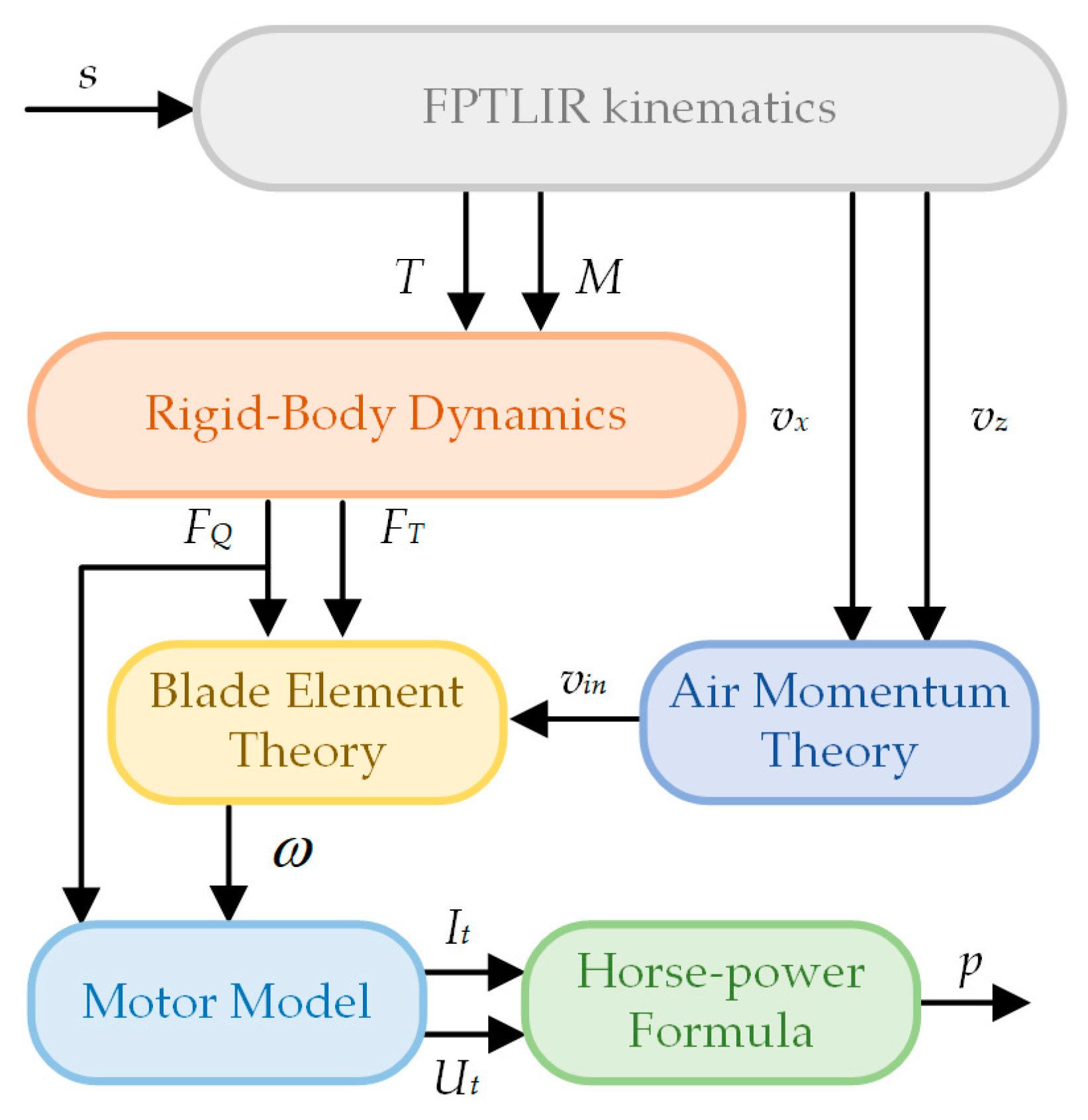
• A mathematical model is constructed to establish a relationship between the mission path and the energy consumption of the FPTLIR. This model takes into account a continuous derivation of the FPTLIR kinematics to the motor dynamics of the end effector and incorporates theories on blade units and aerodynamics. By considering these factors simultaneously, the accuracy and suitability of the model is improved, making it suitable for building a multiobjective optimization model;
• An optimization model is developed with energy consumption and time as objectives, based on the energy consumption model. Complex constraint indices such as stability and safety during the FPTLIR missions are quantified and considered in the model. The influence of the uniform variable velocity flight state phase on energy consumption is also considered. This improves the adaptability of the model to actual mission requirements;
• An optimization approach is proposed for energy consumption and execution time during the FPTLIR’s both on-line and off-line mission paths. The approach uses an improved NSGA-II optimization algorithm that incorporates concepts from the Cauchy variation operator and the simulated annealing algorithm. This improvement improves the robustness and local search capability of the algorithm under complex constraints. In addition, the proposed approach effectively reduces energy consumption and ensures the shortest mission execution time under the corresponding energy consumption.

The rest of this paper is organized as follows. Section 2 gives an overview of the FPTLIR system. Section 3 presents the inspection requirements and the working principle of the FPTLIR. Section 4 constructs an energy consumption model for the flight system, which establishes a relationship between the mission paths and the energy consumption of the FPTLIR. In Section 5, a multiobjective optimization is performed using the improved NSGA-II implemented in MATLAB, followed by an analysis of the optimization results. Section 6 conducts parameter measurement fitting tests and model prediction accuracy validation tests for the energy model using a test platform, followed by validation of the multiobjective optimization results using the Simulink simulation platform. Section 7 discusses the limitations and perspectives of the method. The final section presents relevant conclusions.

2. System Overview

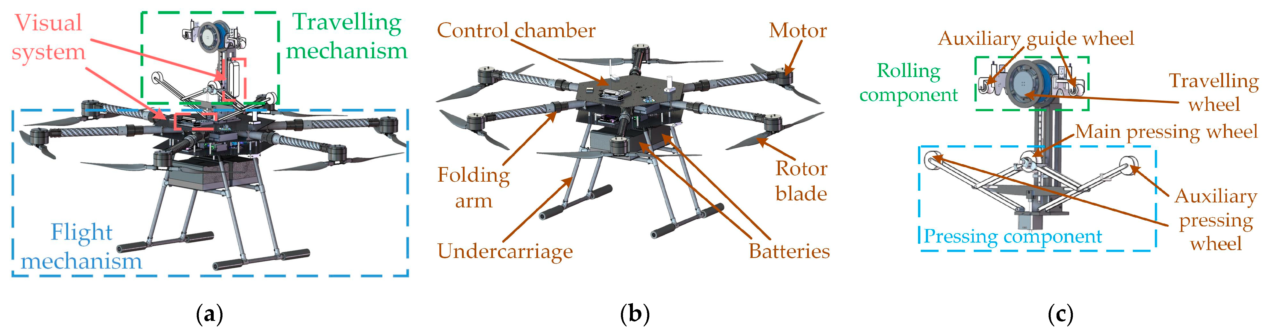
2.1. System Structure

The configuration of the FPTLIR is shown in Figure 1, which consists of two main components: the flight mechanism and the travelling mechanism [39]. The flight mechanism is designed according to a hexacopter UAV, which includes the undercarriage, folding arm, control chamber, motor, and rotor blade. In addition, the travelling mechanism consists mainly of rolling components and pressing components. The rolling component comprises an active travelling wheel and two auxiliary guide wheels, while the pressing component includes a main pressing wheel and two auxiliary pressing wheels. Moreover, two lithium–polymer batteries are located under the control chamber to adjust the FPTLIR’s center of gravity for improved flight stability.

2.2. Hardware Integration

The FPTLIR is equipped with two lithium batteries that power its various systems for normal operation. These systems include the flight system, travelling and pressing system, vision system, and other sensors, as shown in Figure 2. The flight system primarily executes the flight function of the FPTLIR to accomplish missions both on-line and off-line. The flight component serves as the driving unit of the flight system, generating the lift for the FPTLIR by rotating the rotor motors in both clockwise and counterclockwise directions to drive the blades, which has an integrated electronic velocity controller. GPS is the position sensor used to obtain the position information of the FPTLIR. The data transmitter is a device that enables the transmission of flight data. The flight controller serves as the control unit of the flight system and contains sensors such as barometers, accelerometers, and others. It analyzes pre-set flight state data and converts them into velocity control commands transmitted to the Electronic Speed Controller (ESC), which controls the speed of the rotor motors. After completing the on-line mission, the FPTLIR relies on rolling components to hang onto the power line. The FPTLIR uses an STM32 microcontroller to control the travelling motor that drives the active travelling wheel, allowing it to move along the power lines. The STM32 can also control the pressing motor to adjust the force between the main pressing wheel, power line, and rolling component to prevent slippage during travel on power lines. The machine’s vision system plays an important role in identifying and detecting power lines and fixtures. It consists of two cameras that capture images, a vision processor that processes the image data, and an image transmitter that facilitates transmission back to the host computer.

This paper focuses on the energy consumption and execution time of the FPTLIR during flight missions. In this case, the flight system operates normally while the traveling and pressing system is in standby mode, requiring only minimal energy supply. It is important to mention that the energy usage of the vision system is quite low compared to the energy requirements of flight missions. Therefore, in the following sections, the static energy consumption is used to estimate the energy usage of the travelling and pressing systems, together with the vision system.

3. Operational Criteria

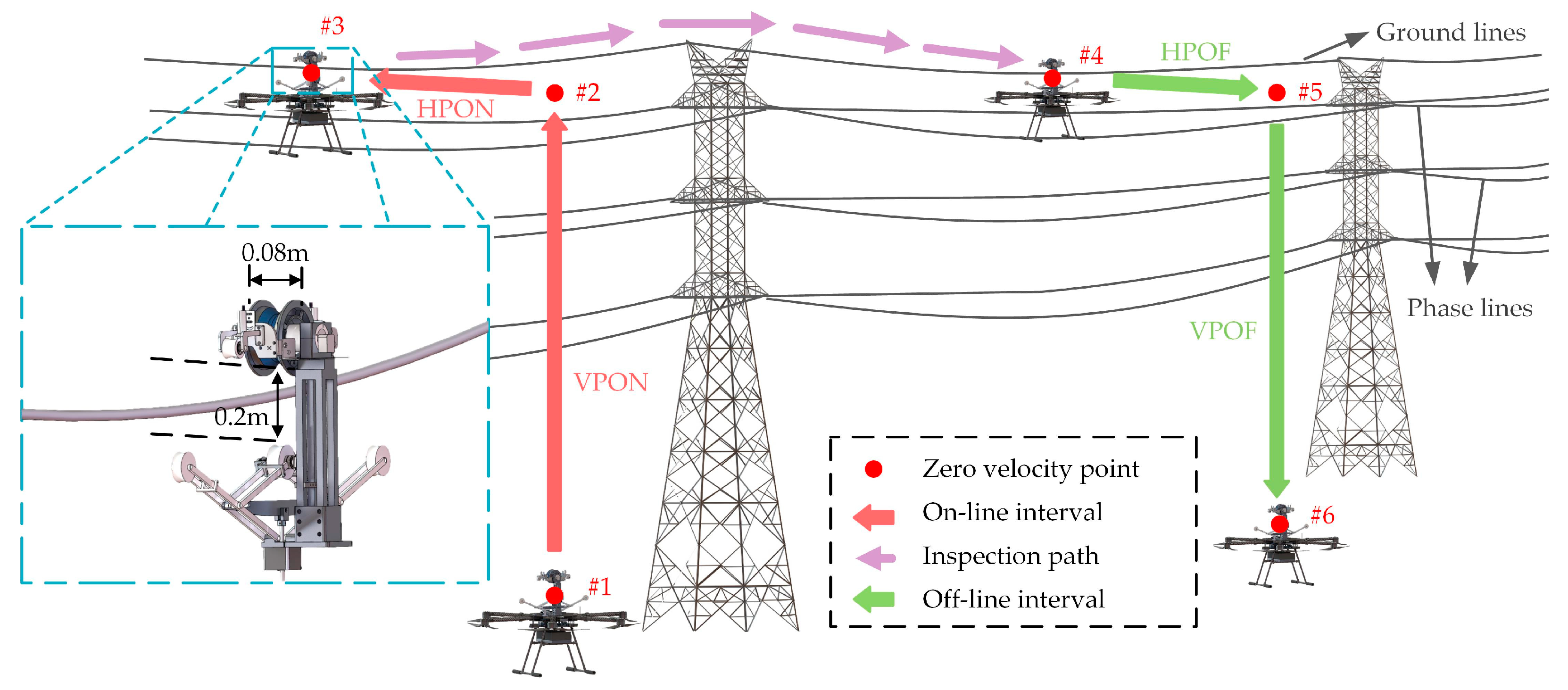
3.1. Working Conditions

Power transmission lines are commonly installed in a variety of terrains and natural environments, leading to a complex and diverse operational setting for the FPTLIR. The tower is a key structure that supports the cables required for power transmission. The levels of transmission lines, tower types, voltage levels, terrain characteristics, and other factors can influence parameters such as the vertical spacing of the transmission line and the height of the lowest point of the ground line. These parameter variations directly affect the energy consumption of the FPTLIR during missions. Therefore, the FPTLIR must have stable flight capabilities and sufficient electrical power to inspect pylons and power lines with varying parameter levels based on the actual requirements. Before each mission, it is necessary to determine the relevant data on the characteristics of these transmission lines.

Table 1. Data on common transmission lines.

Transmission Line Voltage Level (kV)	Tower Height (m)	Vertical Clearance (m)	Ground Wire Height from Ground (m)
110	15–25	2–3	10–20
220	30–40	3–4	20–30
330	35–60	4–5	25–35
550	45–75	5–6	30–40
750	65–100	6–7	40–50
1000	75–120	7–8	45–55

lists some common data for reference.

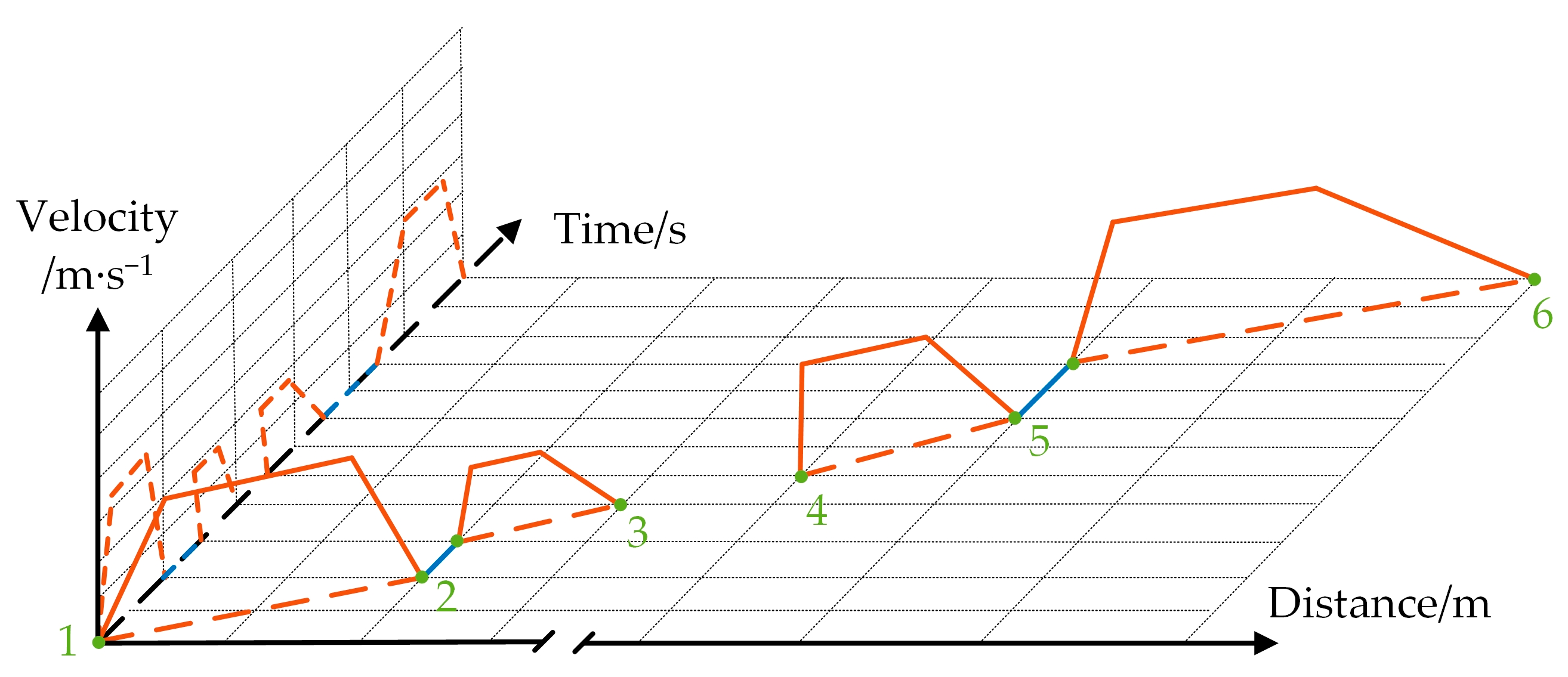
3.2. Mission Path Planning

The landing point for the FPTLIR flight on-line and off-line missions is the lowest point along the ground line of the transmission line. It is important to consider potential electromagnetic interference from the phase lines under the ground lines when planning the mission path. This requires selecting safe vertical and horizontal flight trajectories and adjusting distances based on parameters such as transmission line height. The complete flight missions of the FPTLIR involves two mission intervals: an on-line interval (#1, 2, 3) and an off-line interval (#4, 5, 6). The on-line interval includes three zero-speed Points (#1), (#2), and (#3) where the robot hovers, and the off-line interval consists of three zero-speed Points (#4), (#5), and (#6). Figure 3 shows the operational path of the FPTLIR, which includes four path intervals within these mission intervals: vertical path interval on-line (VPON), horizontal path interval on-line (HPON), horizontal path interval off-line (HPOF), and vertical path interval off-line (VPOF).

The FPTLIR takes off vertically from a secure ground Point (#1) and ascends to Point (#2), determined by the parameters of the currently inspected transmission line. At Point (#2), the vertical positional accuracy error is maintained within ±0.1 m to ensure that the ground line remains safely positioned between the active walking wheel and the main pressure wheel. After briefly hovering, the FPTLIR continues to fly horizontally towards the ground line until it reaches Point (#3). At Point (#3), it is important to ensure that the ground line is aligned with the notch of the active travelling wheel and is slightly lower than the wheel. Therefore, the horizontal position error should be maintained within ±0.04 m, which is equivalent to the width of the notch on the active travelling wheel. The FPTLIR flies down a very short distance and lands on the power line, after which it turns on the travelling system and starts walking along the power line for inspection work. Upon completion of the multi-stage inspection mission, the travelling system is switched off, and the flight system is activated. The FPTLIR will ascend a short distance, detach from the power lines, and hover at Point (#4). Afterward, the FPTLIR flies backward horizontally towards Point (#5). At this point, the position accuracy should be within ±0.04 m to ensure landing in the safe landing zone. After a short hover period at this position, the FPTLIR descends vertically until reaching a secure landing spot at Point (#6), allowing for a maximum allowable error of −0.1 m. Among them, the flight distance during the stages of landing on and detaching from power lines is extremely short and the hovering time at Points (#2) and (#4) is very short, resulting in negligible energy consumption. Therefore, we will exclude the energy consumption analysis during these stages.

4. Energy Consumption Modeling

4.1. Subsystem Model

An inertial reference frame $\{{\mathit{e}}_{\mathbf{1}},{\mathit{e}}_{\mathbf{2}},{\mathit{e}}_{\mathbf{3}}\}$ is initially established, followed by consideration of the fuselage of the FPTLIR as a rigid body to establish a rigid coordinate system $\{{\mathit{b}}_{\mathbf{1}},{\mathit{b}}_{\mathbf{2}},{\mathit{b}}_{\mathbf{3}}\}$, with the origin positioned at the center of gravity. Here, ${\mathit{b}}_{\mathbf{1}}$ and ${\mathit{b}}_{\mathbf{2}}$ denote the forward and upward directions of the FPTLIR, respectively, while ${\mathit{b}}_{\mathbf{3}}$ can be determined using the right-hand rule. Figure 4 shows the coordinate system and force analysis of the FPTLIR, while its rigid-body dynamics equations in 3D space are presented as Equations (1)–(3).

$$m\ddot{\mathit{s}}={\mathit{T}}_{n}R{\mathit{e}}_{\mathbf{3}}-mg{\mathit{e}}_{\mathbf{3}}-\frac{1}{2}\rho S_E‖\dot{\mathit{s}}‖\dot{\mathit{s}}$$

(1)

$$J\dot{\mathbf{\Omega }}={\rm M}-\mathbf{\Omega }\times J\mathbf{\Omega }$$

(2)

$$\dot{R}=R\widehat{\mathbf{\Omega }}$$

(3)

where $m$ is the mass of the FPTLIR, ${\mathit{T}}_n$ is the net thrust of the FPTLIR, $R$ is the rotation matrix of the rigid-body coordinate system mapped to the inertial reference system, $g$ is the acceleration of gravity, $\rho$ is the density of the air at $25 ℃$, $S_E$ is the equivalent planar area of the fuselage ($S_E$ is equal to $S_{HE}$ for horizontal flight of the FPTLIR, and is equal to and $S_{VE}$ for vertical flight), $\mathit{s}$ is the path position of the FPTLIR in the inertial coordinate system $\left\{\mathit{e}\right\}$, $J$ is the inertia matrix and $J=diag[I_x,I_y,I_z]$, and $\mathbf{\Omega }\in {ℝ}^3$ is the angular velocity of the FPTLIR in the rigid-body coordinate system. Operator $\wedge$ is defined as follows: for any $x,y\in {ℝ}^3$, there exists $\widehat{x}y=x\times y$. The operator $\vee$ is the inverse of operator $\wedge$.

The net thrust and combined moment required for the FPTLIR to follow a given path ${\mathit{s}}_{\mathit{g}}$ can be determined using Equations (4) and (5), respectively.

$${\mathit{T}}_{\mathit{n}\mathit{g}}=m{\ddot{\mathit{s}}}_{\mathit{g}}+mg{\mathit{e}}_{\mathbf{3}}+\frac{1}{2}\rho S_E‖{\dot{\mathit{s}}}_{\mathit{g}}‖{\dot{\mathit{s}}}_{\mathit{g}}$$

(4)

$${\mathit{M}}_{\mathit{g}}=J{\dot{\mathbf{\Omega }}}_{\mathit{g}}+{\mathbf{\Omega }}_{\mathit{g}}\times J{\mathbf{\Omega }}_{\mathit{g}}$$

(5)

where ${\mathbf{\Omega }}_{\mathit{g}}={(R_g^T{\dot{R}}_g)}^{\vee }$, and the derivation of ${\mathbf{\Omega }}_{\mathit{g}}$ yields ${\dot{\mathbf{\Omega }}}_{\mathit{g}}={({\dot{R}}_g^T{\dot{R}}_g+R_g^T{\ddot{R}}_g)}^{\vee }$. As the thrust direction of the FPTLIR always aligns with the ${\mathit{b}}_{\mathbf{3}\mathit{g}}$ axis in the rigid-body coordinate system, it can be inferred that ${\mathit{b}}_{\mathbf{3}\mathit{g}}={\mathit{T}}_{\mathit{n}\mathit{g}}/‖{\mathit{T}}_{\mathit{n}\mathit{g}}‖$. Similarly, since the velocity direction aligns with the ${\mathit{b}}_{\mathbf{1}\mathit{g}}$ axis, it can be deduced that ${\mathit{b}}_{\mathbf{1}\mathit{g}}={\dot{\mathit{s}}}_{\mathit{g}}/‖{\dot{\mathit{s}}}_{\mathit{g}}‖$. Finally, the application of the right-hand rule leads to the determination of the last axis as ${\mathit{b}}_{\mathbf{2}\mathit{g}}={\mathit{b}}_{\mathbf{3}\mathit{g}}\times {\mathit{b}}_{\mathbf{1}\mathit{g}}$. Thus, the rotation matrix is expressed by Equation (6).

$${\mathit{R}}_{\mathit{g}}=[{\mathit{b}}_{\mathbf{1}\mathit{g}},{\mathit{b}}_{\mathbf{2}\mathit{g}},{\mathit{b}}_{3g}]$$

(6)

After calculating the first and second order derivatives of the rotation velocity matrix, ${\dot{\mathit{R}}}_{\mathit{g}}$ and ${\ddot{\mathit{R}}}_{\mathit{g}}$ can be obtained. Substituting them into Equation (5), the required combined moment ${\mathit{M}}_{\mathit{g}}$ is determined. Through this deduction, the net thrust and combined torque required to achieve the corresponding motion can be obtained from the path. The FPTLIR adjusts the magnitude of the angular velocity of all six propellers to change both the generated thrust and torque accordingly. Neglecting the precision errors due to elastic deformation and friction between blades and fuselage, Equations (7)–(10) demonstrate how the net thrust and the torque are calculated through rigid-body dynamics of the FPTLIR.

$$T_n={\displaystyle \sum _{i=1}^6{F}_{Ti}}$$

(7)

$$M_1=\frac{1}{2}l(-F_{T1}-F_{T3}+F_{T4}+F_{T6})+l(-F_{T2}+F_{T5})$$

(8)

$$M_2=\frac{\sqrt{3}}{2}l(-F_{T1}+F_{T3}+F_{T4}-F_{T6})$$

(9)

$$M_3=F_{Q1}-F_{Q2}+F_{Q3}-F_{Q4}+F_{Q5}-F_{Q6}$$

(10)

where $F_{Ti}$($i=1,\dots ,6$) is the individual thrust generated by each of the six propellers’ rotations. $M_1$, $M_2$, and $M_3$ represent moments around the axes ${\mathit{b}}_{\mathbf{1}}$, ${\mathit{b}}_{\mathbf{2}}$, and ${\mathit{b}}_{\mathbf{3}}$, respectively. The combined moment is denoted as $\mathit{M}=[M_1,M_2,M_3]$. $F_{Qi}$($i=1,\dots ,6$) is the torque produced by each propeller’s rotation. Additionally, $l$ refers to the distance between the center of gravity of the FPTLIR and its propellers’ center.

The thrust and torque of a single power unit of the FPTLIR can be determined by the propeller aerodynamics. The model consists of two components: one based on the blade unit theory, which calculates the propeller’s thrust and torque, and another based on the momentum theory, which calculates the aerodynamics of the propeller inflow. Figure 4 illustrates the force and velocity analyses on the cross-section of the blade. The angle between the blade cross-section’s zero-lift line and the airflow direction is the aerodynamic angle of attack. The lift coefficient is directly proportional to this angle and can be obtained from both the propeller blade’s torsion angle and the incoming flow angle. Following the blade unit theory, Equation (11) is derived to express the lift and drag in a blade section located extremely close to the rotor motor’s axis of rotation.

$$dL=0.5\rho u^{2}ck(\theta (r)-\phi (r))dr,dD=0.5\rho u^{2}c{c}_{d}dr$$

(11)

where $dL$ is the blade unit lift, $u$ is the air inflow velocity, $c$ is the blade chord length, $k$ is the linearity coefficient, $\theta$ is the twist angle of the blade, $\phi$ is the airflow incidence angle ($\theta$ and $\phi$ vary with $r$), $dD$ is the drag, $c_d$ is the drag coefficient (normally the coefficient of drag is considered constant), and $r$ is the radial distance of the blade unit from the rotor motor shaft. The horizontal and vertical components of the FPTLIR’s airspeed can be determined by coordinate transformations, as shown in Equation (12), when the FPTLIR is flying at a given speed.

$$v_x=(V+V_w)R^{-1}{\mathit{e}}_{\mathbf{1}},v_z=(V+V_w)R^{-1}{\mathit{e}}_{\mathbf{3}}$$

(12)

where $v_x$ is the horizontal component of the airspeed relative to the fuselage rigid body, $v_z$ is the vertical component of the airspeed relative to the fuselage rigid body, $V_w$ is the wind speed in the inertial reference frame, $R^{-1}$ is the rotation matrix from the inertial reference system to the rigid-body coordinate system, and $V$ is the flight velocity of the FPTLIR in the inertial coordinate system. As depicted in Figure 4, the airflow incidence angle and the airspeed can be derived from the horizontal and vertical components of the airspeed, which are calculated according to Equation (13).

$$\begin{array}{l}{u}_{pl}(r,\psi )=\omega r+v_x\sin (\psi )\\ u_{pr}(r)=v_{in}+v_z\\ u(r,\psi )=\sqrt{u_{pl}{}^2+u_{pr}{}^2}\\ \phi (r,\psi )={\tan }^{-1}(u_{pr}/u_{pl})\end{array}$$

(13)

where $\omega$ is the angular velocity of the propeller, $v_{in}$ is the air induced velocity, $u_{pl}$ is the horizontal component of the air inflow velocity $u$, $u_{pr}$ is the vertical component of the air inflow velocity $u$, and $\psi$ is the angular position of the propeller blade in the direction of rotation. According to the force analysis shown in Figure 4, the thrust and torque acting on the blade unit cross-section can be calculated using Equation (14).

$$\begin{array}{l}d{F}_T\left(r,\psi \right)=N\left(dL\cos \phi -dD\sin \phi \right)\\ d{F}_Q\left(r,\psi \right)=Nr\left(dL\cos \phi +dD\sin \phi \right)\end{array}$$

(14)

where $N$ is the number of blades of the propeller. Considering that the horizontal component of the airflow incidence velocity typically greatly exceeds its vertical counterpart, and given that the drag force is generally perpendicular to the thrust direction and considerably less than the lift force, it is common practice to ignore the reverse drag component in the calculated torque equation. The determination of the propeller thrust and torque involves integrating the solution and averaging over one rotation cycle of the propeller in Equation (15).

$$\begin{array}{l}{F}_{\mathit{T}}={\displaystyle {\int }_{R_1}^{0.97R_2}{\displaystyle {\int }_0^{2\pi }0.5N\rho u_{pl}^{2}ck(\theta -u_{pr}/u_{pl})}}d\psi dr/(2\pi )\\ F_Q={\displaystyle {\int }_{R_1}^{R_2}{\displaystyle {\int }_0^{2\pi }0.5Nr\rho u_{pl}^{2}c(\phi k(\theta -u_{pr}/u_{pl})+c_d)}}d\psi dr/(2\pi )\end{array}$$

(15)

where $R_1$ is the blade bottom length and $R_2$ is the blade length. It should be noted that the thrust of the paddle element is calculated by integration only up to 97% of the paddle blade length, and the tip losses can be approximated to be negligible in this calculation [40].

The wind has a direct effect on the air-induced velocity of the propeller. Applying the blade unit theory and the principles of the air momentum theory to account for the effect of air-induced velocity on the propeller thrust and torque can improve the accuracy of the flight energy consumption model. In order to determine the air-induced velocity, it is necessary to calculate it using the principles of the air momentum theory. As depicted in Figure 4, Point 1 represents the airflow inlet where the relative velocity, i.e., the total air velocity of the FPTLIR, can be obtained by summing up both horizontal and vertical components of air velocities. The airflow is accelerated perpendicular to the plane of propeller rotation, resulting in distinct induced velocities at Point 2 (propeller rotation plane) and Point 3 (airflow outlet). Applying the conservation laws for momentum and kinetic energy, it can be seen that the induced velocity at Point 3 is twice as much as that at Point 2. Through this analysis, a relationship between thrust, airflow mass flow, and induced velocity at the propeller rotation plane can be expressed by Equation (16).

$$\begin{array}{l}\dot{m}=\rho \pi R_2{}^2\sqrt{v_x{}^2+{(v_z+v_{in})}^2}\\ F_{\mathit{T}}=\dot{m}{v}_o=2\dot{m}{v}_{in}=2\rho \pi R_2{}^2{v}_{in}\sqrt{v_x{}^2+{(v_z+v_{in})}^2}\end{array}$$

(16)

where $\dot{m}$ is the mass of air flow, $v_{in}$ is the induced velocity at point 2, and $v_o$ is the induced velocity at point 3. The induced velocity at point 2 can be determined by solving expression (17) as presented as follows.

$$v_{in}^4+2v_z{v}_{in}^3+v^2{v}_{in}^2={(F_T/2\rho \pi R_2{}^2)}^2$$

(17)

Brushless DC rotor motors are used as the end-effector to drive the flight system of the FPTLIR, and improvement of the accuracy of the energy consumption model can be achieved by incorporating their dynamics into the modelling process. As the rotor motor is controlled electronically with a fast response time, transient effects are not considered. The equivalent circuit diagram of the rotor motor is illustrated in Figure 4, and its mathematical representation follows a three-parameter model [41,42]. By combining this with a simplified motor model, Equation (18) can be used to calculate main road currents and voltages applied to the rotor motor.

$$\begin{array}{l}{I}_t=F_Q{K}_V+I_0\\ U_t=\frac{\omega }{K_V}+F_Q{K}_V{R}_m\end{array}$$

(18)

where $I_t$ is the dry circuit current input to the rotor motor, $U_t$ is the dry circuit voltage, $F_Q$ is the load torque of the propeller, $K_V$ is the velocity constant of the rotor motor, $I_0$ is the current required by the rotor motor when the load on the rotor motor is zero, and other losses of the rotor motor such as friction losses and magnetic losses are included in the no-load current $I_0$ of the rotor motor. $\omega$ is the angular velocity of the rotor motor and the paddle, and $R_m$ is the resistance of the rotor motor winding. The relationship between the path and the voltage and current of the end effector can be described by the above derivation.

4.2. System Model

Finally, the relationship between path trajectories and the FPTLIR energy consumption is established after a series of modelling derivations. The transfer of relationships between the sub-models is shown in Figure 5.

The power of a single rotor motor can be expressed by Equation (19).

$$p(t)=U_t(t)I_t(t)$$

(19)

where $p(t)$ is the power of a single rotor motor. The total energy consumption of the FPTLIR during the flight time T can be determined by Equation (20).

$$W(t)={\displaystyle {\int }_0^{\mathit{T}}P(t)dt}$$

(20)

where $W(t)$ is the total energy consumed by the FPTLIR during the flight time T, and $P(t)={\displaystyle \sum _{i=1}^6{p}_i(t)}$ signifies the aggregate power generated by all six rotor motors of the FPTLIR.

5. Multiobjective Optimization Approach

5.1. Multiobjective Optimization Modeling

5.1.1. Mission Path Model

The optimization of the FPTLIR flight energy consumption model for multiobjective purposes in both on-line and off-line mission paths consists of two main components: velocity curve optimization and time optimization. The main aim of the velocity curve optimization is to reduce the total energy consumption during mission intervals by adjusting the velocity commands of the FPTLIR in each path interval. The time optimization aims to reduce the total flight duration by adjusting the flight time of the FPTLIR in each mission path interval. This paper mainly focuses on reducing the energy consumption of the system while ensuring the shortest mission execution time under the corresponding energy consumption.

A discrete time dimension is introduced to analyze the integrated optimization problem involving the FPTLIR’s flight velocity curves and mission interval time. This extension transforms the physical network into a high-dimensional physical-spatiotemporal network. Figure 6 shows the spatiotemporal variation of the FPTLIR during on-line and off-line missions and depicts two mission intervals (#1,2,3) and (#4,5,6) comprising six zero-velocity Points (#1)–(#6), along with their corresponding discrete spatiotemporal networks. By discretizing the time T axis, Equation (21) represents the duration of these two mission intervals.

$$T=\{t_x+n\tau |x=0,1;n=0,1,\dots ,M\}$$

(21)

wherein $t_x$, when the subscript $x=0,1$ denotes the initial moments of the flight on-line and flight off-line missions, respectively, $n$ is an integer, and $\tau$ is a tiny time increment. The FPTLIR can arrive at the zero-velocity point or leave the zero-velocity point at any discrete moment on the T-axis. The spatiotemporal path $(i,j,t,t^{\prime })$ represents the FPTLIR leaving from point $i$ at moment $t$ and arriving at point $j$ at moment $t^{\prime }$. It is used to represent the spatiotemporal change process of the FPTLIR during the two mission intervals, and the interval flight time required for the process is $t^{\prime }-t$.

The flight mission path can be established after identifying the power lines and towers that need to be inspected. Based on the spatiotemporal network flight path model, the flight velocity curves are incorporated to represent the relationship between flight time and velocity in the FPTLIR mission interval. As shown in Figure 7, each spatiotemporal path $(i,j,t,t^{\prime })$ from Figure 6 corresponds to different specific flight velocity curves $\left\{v_{ijt{t}^{\prime }}\right|t<x<t^{\prime }\}$, thus forming a three-dimensional coordinate system for the FPTLIR’s flight velocity curve.

It is essential to optimize the flight state of the FPTLIR within each path interval to achieve the objective of energy and time conservation. The four path intervals are divided into state intervals based on different flight states, and the precision of these intervals significantly affects both optimization speed and effectiveness. Increasing the number of state intervals may improve the optimization results, but may lead to frequent flight state transitions that do not meet the stability requirements of the FPTLIR. Therefore, each path interval is divided into three sequential state intervals: acceleration, uniform velocity, and deceleration. Energy-saving and time-saving velocity curves can be generated for mission intervals through multiobjective optimization by optimizing eight flight state commands including vertical acceleration magnitude, vertical acceleration time, vertical uniform velocity time, vertical deceleration magnitude, horizontal acceleration magnitude, horizontal acceleration time, horizontal uniform velocity time, and horizontal deceleration magnitude within each path interval. Combined with the previously discussed energy consumption model, the position trajectories of different flight state intervals in VPON, HPON, HPOF, and VPOF can be represented by Equations (22)–(25), respectively.

$${\mathit{s}}_{\mathbf{vn}\mathbf{1}}(t)=[0,0,\frac{1}{2}{a}_{\mathrm{vn}1}{t}_{\mathrm{vn}1}^2],{\mathit{s}}_{\mathbf{vn}\mathbf{2}}(t)=[0,0,v_{\mathrm{vn}}{t}_{\mathrm{vn}2}],{\mathit{s}}_{\mathbf{vn}\mathbf{3}}(t)=[0,0,v_{\mathrm{vn}}{t}_{\mathrm{vn}3}-\frac{1}{2}{a}_{\mathrm{vn}2}{t}_{\mathrm{vn}3}^2]$$

(22)

$${\mathit{s}}_{\mathbf{hn}\mathbf{1}}(t)=[\frac{1}{2}{a}_{\mathrm{hn}1}{t}_{\mathrm{hn}1}^2,0,0],{\mathit{s}}_{\mathbf{hn}\mathbf{2}}(t)=[v_{\mathrm{hn}}{t}_{\mathrm{hn}2},0,0],{\mathit{s}}_{\mathbf{hn}\mathbf{3}}(t)=[v_{\mathrm{hn}}{t}_{\mathrm{hn}3}-\frac{1}{2}{a}_{\mathrm{hn}2}{t}_{\mathrm{hn}3}^2,0,0]$$

(23)

$${\mathit{s}}_{\mathbf{hf}\mathbf{1}}(t)=[\frac{1}{2}{a}_{\mathrm{hf}1}{t}_{\mathrm{hf}1}^2,0,0],{\mathit{s}}_{\mathbf{hf}\mathbf{2}}(t)=[v_{\mathrm{hf}}{t}_{\mathrm{hf}2},0,0],{\mathit{s}}_{\mathbf{hf}\mathbf{3}}(t)=[v_{\mathrm{hf}}{t}_{\mathrm{hf}3}-\frac{1}{2}{a}_{\mathrm{hf}2}{t}_{\mathrm{hf}3}^2,0,0]$$

(24)

$${\mathit{s}}_{\mathbf{vf}\mathbf{1}}(t)=[0,0,\frac{1}{2}{a}_{\mathrm{vf}1}{t}_{\mathrm{vf}1}^2],{\mathit{s}}_{\mathbf{vf}2}(t)=[0,0,v_{\mathrm{vf}}{t}_{\mathrm{vf}2}],{\mathit{s}}_{\mathbf{vf}3}(t)=[0,0,v_{\mathrm{vf}}{t}_{\mathrm{vf}3}-\frac{1}{2}{a}_{\mathrm{vf}2}{t}_{\mathrm{vf}3}^2]$$

(25)

where ${\mathit{s}}_{\mathit{x}\mathit{y}\mathit{m}}$, ${\mathit{t}}_{\mathit{x}\mathit{y}\mathit{m}}$, ${\mathit{a}}_{\mathit{x}\mathit{y}\mathit{k}}$, and ${\mathit{v}}_{\mathit{x}\mathit{y}}$ are the parameters in the four path intervals VPON, HPON, HPOF, and VPOF. Here, the term $\mathit{s}$ is the path of the interval position, $t$ is the duration of the flight state interval, $a$ is the acceleration of the uniformly variable velocity, and $v$ indicates uniform velocity. The subscript $x=\mathsf{v},\mathsf{h}$ denotes vertical and horizontal paths, respectively; $y=\mathsf{n},\mathsf{f}$ denotes on-line and off-line paths, respectively; $m=1,2,3$ denotes acceleration, uniform velocity, and deceleration intervals, respectively; while $k=1,2$ denotes acceleration and deceleration intervals, respectively.

5.1.2. Constraints and Objective Functions

Based on the design specifications and performance data of the FPTLIR, we carried out a comprehensive evaluation of its working conditions. To meet stability and safety requirements, kinematic constraints such as acceleration and velocity limitations need to be implemented. The maximum achievable horizontal acceleration for the FPTLIR is 10 m/s², while the maximum vertical acceleration is 6 m/s². Equation (26) is the expression of these acceleration constraints.

$$\left\{\begin{array}{l}0<a_{\mathrm{hn}1},a_{\mathrm{hn}2},a_{\mathrm{hf}1},a_{\mathrm{hf}2}\le 10\mathsf{m}/{\mathsf{s}}^2\\ 0<a_{\mathrm{vn}1},a_{\mathrm{vn}2},a_{\mathrm{vf}1},a_{\mathrm{vf}2}\le 6\mathsf{m}/{\mathsf{s}}^2\end{array}\right.$$

(26)

FPTLIR has different upper limits for flight speed in various modes, and Equation (27) represents these limits.

$$\left\{\begin{array}{l}0\le v\le v_{\lim }\\ v_{\lim }=\left\{v_{\mathrm{ascent}\_\max },v_{\mathrm{descent}\_\max },v_{\mathrm{horizontal}\_\max }\right\}\end{array}\right.$$

(27)

where $v$ is the flight velocity of the FPTLIR, $v_{\lim }$ is the maximum velocity limit, the maximum ascent velocity $v_{\mathrm{ascent}\_\max }$ = 10 m/s, the maximum descent velocity $v_{\mathrm{descent}\_\max }$ = 7 m/s, and the maximum horizontal flight velocity $v_{\mathrm{horizontal}\_\max }$ = 16.8 m/s. According to the preceding section, it is evident that the instantaneous velocity of the FPTLIR at both its arrival and departure from the point of zero velocity is 0, which must adhere to the constraints presented in Equation (28).

$$v_{{ijtt}^{\prime }}(t)=v_{{ijtt}^{\prime }}(t^{\prime })=0$$

(28)

The position accuracy metrics should be considered to ensure the success of both on-line and off-line missions. Specifically, these metrics need to be evaluated when the FPTLIR flight reaches the zero-velocity point, and their constraints can be expressed as follows:

$$\left\{\begin{array}{l}\left|S-S_{\mathrm{target}x}\right|\le K_x;(x=1,2,3)\\ K_4\le S-S_{\mathrm{target}4}\end{array}\right.$$

(29)

where $S$ is the total flight distance under the flight path interval, $S_{\mathrm{target}x}$ is the ideal zero-velocity point location distance under different flight path intervals, which is determined by the parameters of the power line to be inspected, $S_{\mathrm{target}1}$ is the ideal vertical flight distance at Point (#2), $S_{\mathrm{target}2}$ is the ideal horizontal flight distance at Point (#3), $S_{\mathrm{target}3}$ is the ideal horizontal flight distance at Point (#5), and $S_{\mathrm{target}4}$ is the ideal vertical flight distance at Point (#6). Correspondingly, $K_x$ is the maximum allowable error, as shown in Figure 3, the maximum allowable errors at Points (#2) and (#3) in the on-line mission interval are $K_1=0.1\mathsf{m}$ and $K_2=0.04\mathsf{m}$, respectively, and the maximum allowable errors at Points (#5) and (#6) in the off-line mission interval are $K_3=0.04\mathsf{m}$ and $K_4=-0.1\mathsf{m}$. The optimization objective of the multiobjective optimization model is to achieve energy and time savings. The optimization model uses the energy consumption index from Section 3 as its objective function, presented in Equation (30).

$$\begin{array}{l}\left\{\begin{array}{l}{f}_{\mathrm{on}1}(a,v,t)=W_1(t)\\ W_1(t)={\displaystyle \sum _{i=1}^3(W_{\mathrm{vn}i}+W_{\mathrm{hn}i})}\end{array}\right.\\ \left\{\begin{array}{l}{f}_{\mathrm{off}1}(a,v,t)=W_2(t)\\ W_2(t)={\displaystyle \sum _{i=1}^3(W_{\mathrm{hf}i}+W_{\mathrm{vf}i})}\end{array}\right.\end{array}$$

(30)

where $W_1$ is the total energy consumption of the FPTLIR in the flight on-line mission interval, $W_2$ is the total energy consumption of the FPTLIR in the flight off-line mission interval, and $W_{\mathrm{vn}i}$, $W_{\mathrm{hn}i}$, $W_{\mathrm{hf}i}$, and $W_{\mathrm{vf}i}$ when subscript $i$ = 1, 2, 3 are the energy consumptions of the FPTLIR in the acceleration, uniformity, and deceleration intervals of the four path intervals of the FPTLIR in the order of priority: the VPON, the HPON, the HPOF, and the VPOF, respectively. The time-saving metric ensures the shortest mission execution time under the corresponding energy consumption in both the on-line and off-line flight intervals as well as meeting the specified time requirements. Equation (31) includes the objective function of the flight time for both on-line and off-line mission intervals, along with the constraints on flight time within these intervals.

$$\begin{array}{l}\left\{\begin{array}{l}{f}_{\mathrm{on}2}(t)={\displaystyle \sum _{i=1}^3(t_{\mathrm{vn}i}+t_{\mathrm{hn}i})}\\ {\displaystyle \sum _{i=1}^3(t_{\mathrm{vn}i}+t_{\mathrm{hn}i})}\le t_{\mathrm{on}}\end{array}\right.\\ \left\{\begin{array}{l}{f}_{\mathrm{off}2}(t)={\displaystyle \sum _{i=1}^3(t_{\mathrm{vf}i}+t_{\mathrm{hf}i})}\\ {\displaystyle \sum _{i=1}^3(t_{\mathrm{vf}i}+t_{\mathrm{hf}i})}\le t_{\mathrm{off}}\end{array}\right.\end{array}$$

(31)

In this case, the total time for the FPTLIR to complete the on-line mission is maximized to $t_{\mathrm{on}}$ = 20 s and the total time to complete the off-line mission is maximized to $t_{\mathrm{off}}$ = 30 s, according to the inspection requirements. The performance indicators mentioned above are quantified as constraints and optimization objectives in the optimization model based on the flight energy model. Each performance index has a distinct focus depending on specific missions. In this paper, the main focus is on the reduction of the mission execution time while ensuring stability and safety indices, position accuracy index, and energy saving.

5.1.3. Optimization Model

To construct a multiobjective optimization model based on the flight energy model, we need to make some assumptions. These are:

• The mission path parameters, FPTLIR performance, and other characteristics are known;
• There are no obstacles or wind disturbances along the FPTLIR’s mission path;
• The power consumption of the onboard auxiliary equipment for the FPTLIR remains constant throughout the mission. This paper aims to address the issue of energy consumption and mission execution time in the FPTLIR during two different mission intervals of on-line and off-line missions.

We establish separate multiobjective optimization models for on-line and off-line mission intervals, considering several indicators such as stability, safety, position accuracy, energy consumption, and time savings. The comprehensive multiobjective optimization model for the on-line mission interval is presented in Equations (32)–(36).

$$\min f(a_{\mathrm{vn}1},t_{\mathrm{vn}1},t_{\mathrm{vn}2},a_{\mathrm{vn}2},a_{\mathrm{hn}1},t_{\mathrm{hn}1},t_{\mathrm{hn}2},a_{\mathrm{hn}2})=\min [f_{\mathrm{on}1}(a,v,t),f_{\mathrm{on}2}(t)]$$

(32)

The objective function is expressed in Equation (33).

$$\begin{array}{l}\left\{\begin{array}{l}{f}_{\mathrm{on}1}(a,v,t)=W_1(t)\\ W_1(t)={\displaystyle \sum _{i=1}^3(W_{\mathrm{vn}i}+W_{\mathrm{hn}i})}\end{array}\right.\\ \left\{\begin{array}{l}{f}_{\mathrm{on}2}(t)={\displaystyle \sum _{i=1}^3\left(t_{\mathrm{vn}i}+t_{\mathrm{hn}i}\right)}\\ {\displaystyle \sum _{i=1}^3\left(t_{\mathrm{vn}i}+t_{\mathrm{hn}i}\right)}\le t_{\mathrm{on}}\end{array}\right.\end{array}$$

(33)

The acceleration constraint is expressed as follows:

$$\left\{\begin{array}{l}0<a_{\mathrm{vn}1},a_{\mathrm{vn}2}\le 6\mathsf{m}/{\mathsf{s}}^2\\ 0<a_{\mathrm{hn}1},a_{\mathrm{hn}2}\le 10\mathsf{m}/{\mathsf{s}}^2\end{array}\right.$$

(34)

The velocity constraint is formulated in Equation (35).

$$\begin{array}{l}{v}_{\mathrm{vn}}-a_{\mathrm{vn}2}{t}_{\mathrm{vn}3}=v_{\mathrm{hn}}-a_{\mathrm{hn}2}{t}_{\mathrm{hn}3}=0\\ \left\{\begin{array}{l}{v}_{\mathrm{vn}}=a_{\mathrm{vn}1}{t}_{\mathrm{vn}1}=a_{\mathrm{vn}2}{t}_{\mathrm{vn}3}\\ 0\le v_{\mathrm{vn}}\le v_{\mathrm{ascent}\_\max }\\ 0<a_{\mathrm{vn}1}{t}_{\mathrm{vn}1}=a_{\mathrm{vn}2}{t}_{\mathrm{vn}3}\le v_{\mathrm{ascent}\_\max }\\ v_{\mathrm{hn}}=a_{\mathrm{hn}1}{t}_{\mathrm{hn}1}=a_{\mathrm{hn}2}{t}_{\mathrm{hn}3}\\ 0\le v_{\mathrm{hn}}\le v_{\mathrm{horizontal}\_\max }\\ 0<a_{\mathrm{hn}1}{t}_{\mathrm{hn}1}=a_{\mathrm{hn}2}{t}_{\mathrm{hn}3}\le v_{\mathrm{horizontal}\_\max }\end{array}\right.\end{array}$$

(35)

The positional accuracy constraints are defined in Equation (36).

$$\left\{\begin{array}{l}{K}_{\mathrm{stop}}=\left|S_1-S_{\mathrm{target}1}\right|<K_1\\ S_1=\frac{1}{2}{a}_{\mathrm{vn}1}{t}_{\mathrm{vn}1}^2+v_{\mathrm{vn}}{t}_{\mathrm{vn}2}+v_{\mathrm{vn}}{t}_{\mathrm{vn}3}-\frac{1}{2}{a}_{\mathrm{vn}2}{t}_{\mathrm{vn}3}^2\\ K_{\mathrm{stop}}=\left|S_2-S_{\mathrm{target}2}\right|<K_2\\ S_2=\frac{1}{2}{a}_{\mathrm{hn}1}{t}_{\mathrm{hn}1}^2+v_{\mathrm{hn}}{t}_{\mathrm{hn}2}+v_{\mathrm{hn}}{t}_{\mathrm{hn}3}-\frac{1}{2}{a}_{\mathrm{hn}2}{t}_{\mathrm{hn}3}^2\end{array}\right.$$

(36)

Similarly, the comprehensive multiobjective optimization model for the off-line mission interval is presented in Equations (37)–(41).

$$\min f(a_{\mathrm{hf}1},t_{\mathrm{hf}1},t_{\mathrm{hf}2},a_{\mathrm{hf}2},a_{\mathrm{vf}1},t_{\mathrm{vf}1},t_{\mathrm{vf}2},a_{\mathrm{vf}2})=\min [f_{\mathrm{off}1}(a,v,t),f_{\mathrm{off}2}(t)]$$

(37)

The objective function is derived as follows:

$$\begin{array}{l}\left\{\begin{array}{l}{f}_{\mathrm{off}1}(a,v,t)=W_2(t)\\ W_2\left(t\right)={\displaystyle \sum _{i=1}^3\left(P_{\mathrm{hf}i}{T}_{\mathrm{hf}i}+P_{\mathrm{vf}i}{T}_{\mathrm{vf}i}\right)}\end{array}\right.\\ \left\{\begin{array}{l}{f}_{\mathrm{off}2}(t)={\displaystyle \sum _{i=1}^3\left(t_{\mathrm{vf}i}+t_{\mathrm{hf}i}\right)}\\ {\displaystyle \sum _{i=1}^3\left(t_{\mathrm{vf}i}+t_{\mathrm{hf}i}\right)}\le t_{\mathrm{off}}\end{array}\right.\end{array}$$

(38)

The acceleration constraint is expressed in Equation (39).

$$\left\{\begin{array}{l}0<a_{\mathrm{hf}1},a_{\mathrm{hf}2}\le 10\mathsf{m}/{\mathsf{s}}^2\\ 0<a_{\mathrm{vf}1},a_{\mathrm{vf}2}\le 6\mathsf{m}/{\mathsf{s}}^2\end{array}\right.$$

(39)

The velocity constraint is defined in Equation (40).

$$\begin{array}{l}{v}_{\mathrm{hf}}-a_{\mathrm{hf}2}{t}_{\mathrm{hf}3}=v_{\mathrm{vf}}-a_{\mathrm{vf}2}{t}_{\mathrm{vf}3}=0\\ \left\{\begin{array}{l}{v}_{\mathrm{hf}}=a_{\mathrm{hf}1}{t}_{\mathrm{hf}1}=a_{\mathrm{hf}2}{t}_{\mathrm{hf}3}\\ 0\le v_{\mathrm{hf}}\le v_{\mathrm{horizontal}\_\max }\\ 0<a_{\mathrm{hf}1}{t}_{\mathrm{hf}1}=a_{\mathrm{hf}2}{t}_{\mathrm{hf}3}\le v_{\mathrm{horizontal}\_\max }\\ v_{\mathrm{vf}}=a_{\mathrm{vf}1}{t}_{\mathrm{vf}1}=a_{\mathrm{vf}2}{t}_{\mathrm{vf}3}\\ 0\le v_{\mathrm{vf}}\le v_{\mathrm{descent}\_\max }\\ 0<a_{\mathrm{vf}1}{t}_{\mathrm{vf}1}=a_{\mathrm{vf}2}{t}_{\mathrm{vf}3}\le v_{\mathrm{descent}\_\max }\end{array}\right.\end{array}$$

(40)

The positional accuracy constraints are expressed as follows:

$$\left\{\begin{array}{l}{K}_{\mathrm{stop}}=\left|S_3-S_{\mathrm{target}2}\right|<K_3\\ S_3=\frac{1}{2}{a}_{\mathrm{hf}1}{t}_{\mathrm{hf}1}^2+v_{\mathrm{hf}}{t}_{\mathrm{hf}2}+v_{\mathrm{hf}}{t}_{\mathrm{hf}3}-\frac{1}{2}{a}_{\mathrm{hf}2}{t}_{\mathrm{hf}3}^2\\ K_4\le K_{\mathrm{stop}}=S-S_{\mathrm{target}4}\\ S_4=\frac{1}{2}{a}_{\mathrm{vf}1}{t}_{\mathrm{vf}1}^2+v_{\mathrm{vf}}{t}_{\mathrm{vf}2}+v_{\mathrm{vf}}{t}_{\mathrm{vf}3}-\frac{1}{2}{a}_{\mathrm{vf}2}{t}_{\mathrm{vf}3}^2\end{array}\right.$$

(41)

In the optimization process of the model, conflicting objective functions make it difficult to find a single optimal solution that minimizes all objectives simultaneously. To address this, each objective should be designed to achieve the optimal solution that satisfies multiple objectives, known as the Pareto optimal solution in multiobjective optimization problems [43]. In this paper, the improved NSGA-II algorithm was employed to solve the Pareto optimal solution.

5.2. Improved NSGA-II

The NSGA-II is a widely used optimization method, which in this paper shows good robustness and convergence when dealing with optimization problems with complex constraints. According to the “no free lunch” theorem, no algorithm can perform optimally on all problems [44,45]. In this paper, the NSGA-II algorithm is improved by adding the Cauchy variation operator and using the concept of a simulated annealing algorithm while trying to retain the advantages of the NSGA-II. These improvements increase the algorithm’s ability to handle complex constraints, increase its robustness, and improve its local search efficiency, making it more suitable for handling the problems in this paper. This is discussed in more detail in the next section.

5.2.1. Genetic Operators

The operators of genetic algorithms encompass selection, crossover, and mutation. However, the polynomial mutation used in the NSGA-II algorithm is not sufficient to solve the Pareto optimal solution frontier optimization problems with complex constraints. This paper introduces Cauchy variation as a random perturbation to improve the algorithm optimization capability. The stochastic variation operator is presented in Equation (42) below.

$${\mathbf{X}}_{i,G+1}=\left\{\begin{array}{l}{\mathbf{X}}_{i,G}+({\mathbf{X}}^{\vartheta }-{\mathbf{X}}^{\zeta })\cdot C(0,1),d<0.5\\ {\mathbf{X}}_{i,G}+({\mathbf{X}}^{\vartheta }-{\mathbf{X}}^{\zeta })\cdot \sigma ({\eta }_m),\mathrm{others}\end{array}\right.$$

(42)

where ${\mathbf{X}}^{\vartheta }$ and ${\mathbf{X}}^{\zeta }$ are the upper and lower bounds of the variable, $\vartheta \in [0,1]$ is the random number, $C(0,1)$ is the random number obeying the standard Cauchy distribution, and ${\eta }_m$ is the polynomial coefficient of variation.

5.2.2. Local Search using Achievement Scalar Function

The Achievement Scalar Function (ASF) is employed as the evaluation function for local search. It is constructed by using a reference point $\overline{z}$ and a weighting vector $\mathit{\delta }$, which is scalarized to multiple targets. This approach guarantees that some targets which are not dominant in the maximum scalarized value are searched. Equation (43) is the formal representation of this function.

$$\left\{\begin{array}{l}\min f(x)=\max {\mathit{\delta }}_i(f_i(x)-{\overline{z}}_i)+\xi {\displaystyle \sum _{i=1}^m{\mathit{\delta }}_i}(f_i(x)-{\overline{z}}_i),x\in D\\ {\mathit{\delta }}_i=({\delta }_1,{\delta }_2\dots ,{\delta }_k)\\ {\delta }_k=1/(z_i{}^{\max }-z_i{}^{\min })\\ {\overline{z}}_i=\underset{e=1}{\overset{N}{\min }}{f}_i(x_e)\end{array}\right.$$

(43)

where $f(x)$ is the objective function, $D$ is the definition domain of the decision variables, ${\mathit{\delta }}_i$ is the set of parameters used to adjust the weight of each objective function, ${\delta }_k$ is the normalization factor to ensure that the weight of each objective function is within a certain range, $z_i{}^{\max }$ and $z_i{}^{\min }$ are the maximum and minimum values of each objective function, respectively, $f_i(x)$ is the objective function, and the coefficients $\xi$ are any extremely small positive numbers. The algorithm uses the Metropolis criterion to decide whether to accept a suboptimal solution from the parent generation as the initial value for the next generation of the population. This decision is based on an acceptance probability, which can be calculated by Equation (44).

$$P=\left\{\begin{array}{l}1,F(X_{\mathrm{new}})<F(X_{\mathrm{old}})\\ \exp (-\frac{F(X_{\mathrm{new}})-F(X_{\mathrm{old}})}{B{T}_c},F(X_{\mathrm{new}})\ge F(X_{\mathrm{old}})\end{array}\right.$$

(44)

where $P$ is the acceptance probability, $F(X_{\mathrm{new}})$ is the child ASF value, $F(X_{\mathrm{old}})$ is the parent ASF value, $B$ is the Boltzmann constant, and $T_c$ is the current temperature.

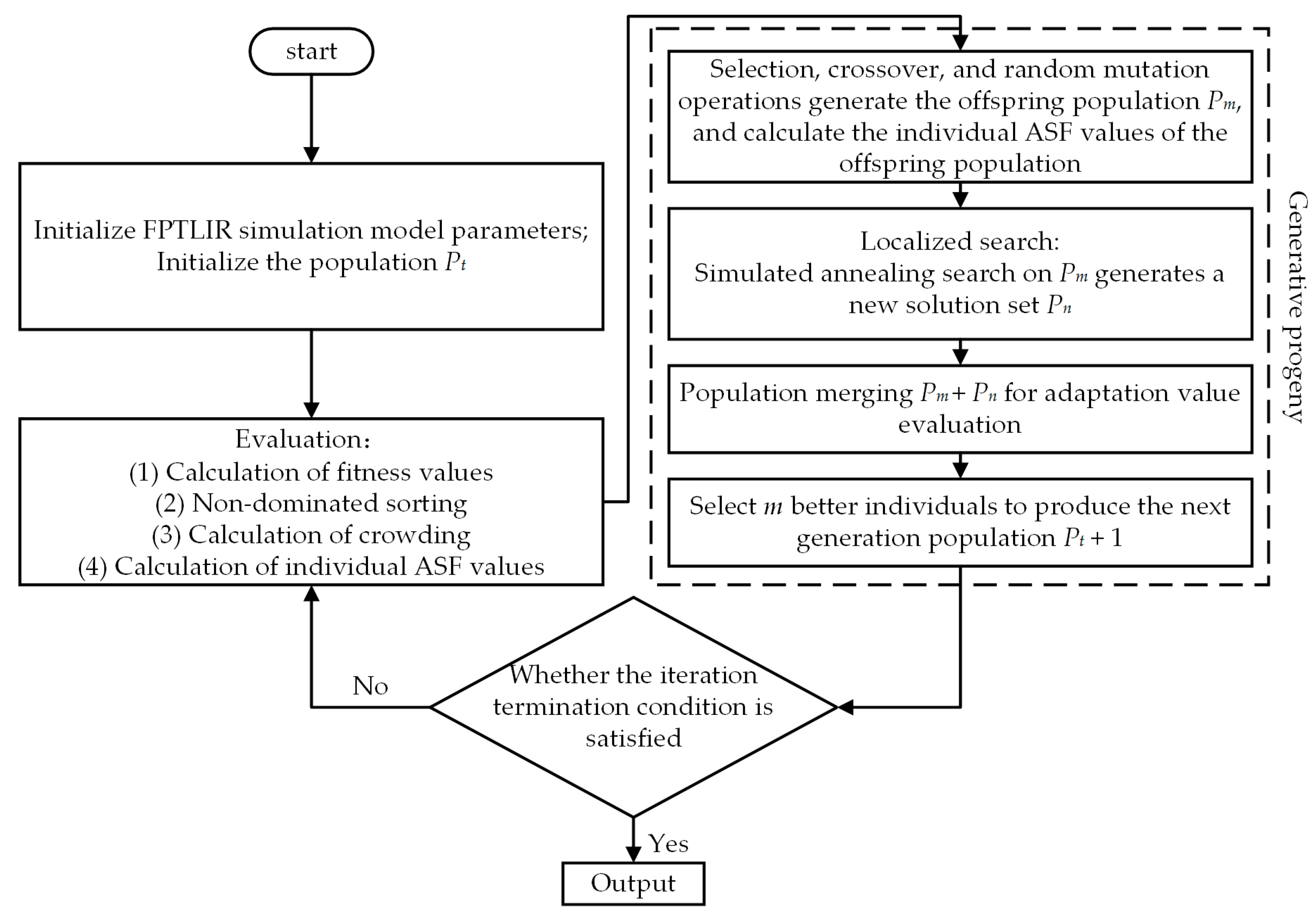
5.2.3. Algorithm Flow

The improved NSGA-II algorithm was used to optimize the FPTLIR’s energy consumption and mission execution time during flight on- and off-line mission paths. The algorithm flowchart is shown in Figure 8.

The algorithm flow is shown as follows:

• Input the parameters of the multiobjective optimization model based on flight energy consumption, including acceleration and velocity constraints, mission interval time constraints, etc. Set algorithm parameters such as iteration number, initial population size, crossover and mutation probabilities, initial temperature, decay coefficient, and final temperature. Initialize the population and calculate objective functions;
• Calculate fitness values for parental individuals using non-dominated sorting and crowding degree calculation methods before calculating the ASF values;
• Generate offspring population $P_m$ by performing crossover and random mutation operations on paternal individuals while also calculating the ASF values for offspring individuals;
• Perform simulated annealing search on the offspring population $P_m$ to compare the parent and offspring ASF values before determining whether to incorporate the new solution set $P_n$ using the Metropolis criterion or to merge with the parent;
• Use the selection operation to determine whether the termination condition or maximum evolutionary generation limit has been reached before outputting results or returning to Step 2.

Algorithm 1 lists the pseudocode of the main process.

Algorithm 1 Improved NSGA-II Algorithm

% Input: Flight energy model parameters and constraints, population size N, % maximum generations T, crossover probability Pc, mutation probability Pm, % initial temperature T0, cooling rate alpha, final temperature Tf % Output: Optimized solution set for energy consumption and mission time % Initialize population for i = 1:N   population(i) = initialize_individual();   [objectives(i), constraints(i)] = evaluate(population(i)); end % Begin evolution t = 0; while t < T   [fronts, ranks] = fast_nondominated_sort(population); % Fast non-dominated sorting   distances = crowding_distance(fronts); % Crowding distance calculation   parents = binary_tournament_selection(population, ranks, distances, Pc); % Selection   children = crossover_and_mutation(parents, Pm); % Crossover and mutation   [objectives_children, constraints_children] = evaluate(children); % Evaluate offspring   [population, ranks] = merge_and_sort(population, children); % Merge and sort   population = elite_selection(population, ranks, distances, N); % Elite selection based on crowding distance   population = asf_local_search(population); % Local search with ASF   population = simulated_annealing(population, T0, alpha); % Simulated annealing decision   T0 = alpha * T0; % Update temperature   t = t + 1; % Increment generation counter end % Output the final solution set optimized_set = population(ranks == 1); % Select the non-dominated set

5.3. Numerical Results of the Algorithm

This paper is based on the actual tower line parameters of 750 KV, where the vertical distance between the lowest point of the ground line and the take-off point of the FPTLIR is 50 m. Additionally, a horizontal distance of 6 m is maintained between the take-off point of the FPTLIR and the plane defined by the ground line during both on-line and off-line missions. The algorithm used in this research was implemented using MATLAB, with optimization results being exported for analysis. Several representative generations were selected to compare convergence effects and optimization results. Figure 9 shows these optimization results over different generations.

It can be observed that the population distributions of the multiobjective optimization for on-line and off-line missions are different in the 1st, 10th, 30th, and 50th generations in Figure 9. As the number of generations increases, both missions show a similar evolutionary pattern in terms of optimization results. In the first generation, the chromosome distribution is more dispersed with some chromosomes positioned further away from the boundary. In addition, the number of chromosomes does not reach the predetermined number of 50, which nevertheless validates the effectiveness of our improved algorithm. By the 10th generation, there is a significant increase in both the quantity and quality of chromosomes, which gradually show regularity and are distributed along the pareto bounds; however, a uniform distribution has not yet been achieved at this stage. By the 30th generation, chromosomes are relatively evenly distributed on Pareto bounds. From the 30th generation to the 50th generation, no significant improvement is observed, indicating convergence of the algorithm by the 30th generation.

Each data point corresponds to a specific combination of flight state command values and energy consumption over time in Figure 9.

Table 2. The flight state commands.

Flight On-Line			Flight Off-Line
Velocity Command	Shortest Flight Time	Post-Optimized	Velocity Command	Shortest Flight Time	Post-Optimized
$a_{\mathrm{vn}1}$	6.00 m/s2	2.17 m/s2	$a_{\mathrm{hf}1}$	10.00 m/s2	0.84 m/s2
$t_{\mathrm{vn}1}$	1.67 s	3.03 s	$t_{\mathrm{hf}1}$	0.77 s	1.41 s
$t_{\mathrm{vn}2}$	3.33 s	4.84 s	$t_{\mathrm{hf}2}$	0	3.99 s
$a_{\mathrm{vn}2}$	6.00 m/s2	2.68 m/s2	$a_{\mathrm{hf}2}$	10.00 m/s2	1.80 m/s2
$a_{\mathrm{hn}1}$	10.00 m/s2	0.35 m/s2	$a_{\mathrm{vf}1}$	6.00 m/s2	0.26 m/s2
$t_{\mathrm{hn}1}$	0.78 s	2.99 s	$t_{\mathrm{vf}1}$	1.17 s	11.56 s
$t_{\mathrm{hn}2}$	0	4.01 s	$t_{\mathrm{vf}2}$	5.96 s	9.88 s
$a_{\mathrm{hn}2}$	10.00 m/s2	2.29 m/s2	$a_{\mathrm{vf}2}$	6.00 m/s2	2.40 m/s2

presents the optimized flight state commands that satisfy all relevant requirements and constraints for both on-line and off-line missions, resulting in the shortest possible flight time and minimum energy consumption. Simulation results and plots have been analyzed to arrive at these commands.

The velocity curves of FPTLIR before and after optimization for both on-line and off-line mission intervals can be obtained from the flight state command. These are shown in Figure 10a and Figure 10b, respectively. Comparing the velocity curves before and after optimization, it can be seen that the FPTLIR performs the acceleration and deceleration actions with smaller acceleration and operates at a lower flight velocity after optimization, considering both the flight energy consumption and time constraints. Based on the simulation results and the 50th generation optimization outcomes, it is determined that the optimal energy consumption for completing the on-line mission in a minimum time of 8.22 s amounts to 1.3750 × 10⁵ J. After optimization, the shortest total time for completing the on-line mission with a minimum energy consumption of 1.3017 × 10⁵ J is found to be 17.77 s, resulting in a significant reduction in energy consumption of about 5.33%. The optimum energy consumption for completing the off-line mission in a minimum time of 9.84 s is estimated to be 1.3667 × 10⁵ J. After optimization, it is found that the total time required to complete the off-line mission with a minimum energy consumption of 1.2983 × 10⁵ J is about 28.78 s, resulting in an effective reduction in energy consumption of about 5.01%. Thus, the objective of reducing the energy consumption of the system and ensuring the shortest mission execution time for the corresponding energy consumption is achieved.

6. Simulation and Test Results

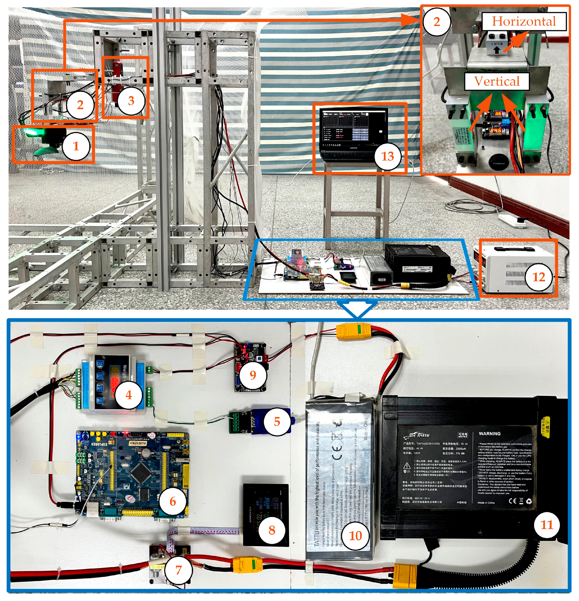
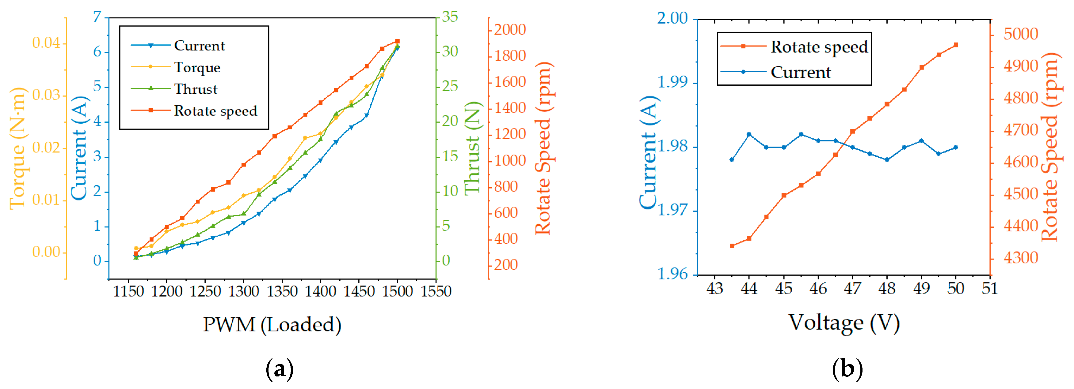
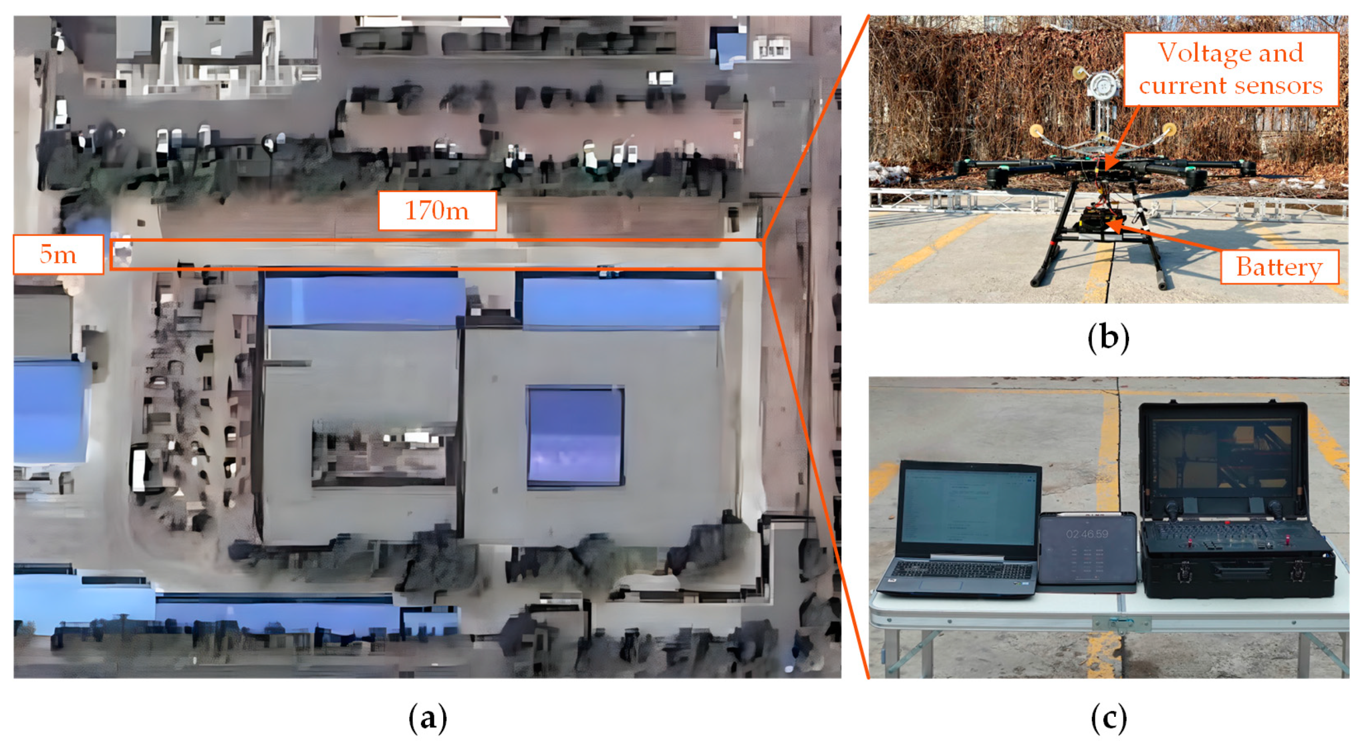
6.1. Parameter Measurement Tests

To determine each model parameter and refine the FPTLIR energy consumption, a test platform was independently designed and built as shown in Figure 11.

The test platform uses an STM32 development board to control both the rotor motor and the blade speed using the PWM signal output from the electronic speed controller. The test platform follows the actual FPTLIR installation method with the rotor motor and blade mounted vertically downwards. A single horizontally mounted parallel beam force sensor is used to measure the thrust generated by the rotor motor and blade rotation, while torque is measured and calculated using two vertically mounted force sensors symmetrically positioned on either side of the rotor motor. A non-contact tachometer is used to measure the speed of both the rotor motor and the blades. Dedicated voltage and current detectors are used for voltage and current measurements, respectively. The power supply for the rotor motor and the electronic speed controller can be either a constant voltage DC power supply or a battery power supply, depending on the actual requirements, with all test data collected and recorded by the upper computer. Detailed design parameters of each sensor in the test platform are listed in

Table 3. Parameters of test platform sensor.

Name	Model	Measuring Range	Precision
Parallel beam force transducer	DLPXL-150	0–30 kg	±0.009 kg
Non-contact tachometer	UT372	10–9999.9 rpm	±0.3 rpm
Current and voltage detector	DT24PW	0–100 A 0–240 V	±0.1 A ±0.01 V

.

To simplify the analysis, we assume that the test platform bracket is stationary and neglect the small deformation caused by the rotation of the rotor motor and paddle. This means that we assume that both the rotor motor and the paddle are in a hovering rotational state. Under this test condition, we can consider $v=v_x=v_z=0$ as the airspeed of the FPTLIR and obtain data under different PWM signals as shown in Figure 12a. Based on these measured data under specified conditions (including load conditions) and combining these with Equation (15), we calculate and fit average values for $k$ to be 5.081 rad⁻¹ and $c_d$ to be 0.005.

In the case where the rotor motor operates without propeller blades and rotates under normal conditions, a series of data was measured, as shown in Figure 12b. Using this data and employing the fitting calculation with the formula $K_V=\omega /U_m$, the speed of the rotor motor is determined to be 100 rpm/V. From Figure 12b, it can be seen that at different voltage values, $I_0$ remains approximately constant at 1.98 A. The comprehensive design parameters and measurement parameters of the FPTLIR are finally obtained as listed in

Table 4. Design parameters and measurement parameters of FPTLIR.

Parameter	Value	Unit
$\mathrm{Chord}\mathrm{length}c(r)$	0.065–0.127r	m
$\mathrm{Twist}\mathrm{angle}\theta (r)$	0.451–1.098r	rad
Air density $\rho$	1.169	kg/m3
Propeller blade number $N$	1
$\mathrm{Length}\mathrm{of}\mathrm{blade}\mathrm{base}{R}_1$	0.073	m
$\mathrm{Length}\mathrm{of}\mathrm{blade}\mathrm{tip}{R}_2$	0.342	m
Linear parameter $k$	5.081	rad−1
$\mathrm{Resistance}\mathrm{coefficient}{c}_d$	0.005
$\mathrm{Motor}\mathrm{resistance}{R}_m$	0.2	Ω
$\mathrm{Zero}\mathrm{load}\mathrm{current}{I}_0$	1.98	A
$\mathrm{Motor}\mathrm{velocity}\mathrm{constant}{K}_V$	100	rpm/V
Rotor location $l$	0.821	m
Mass $m$	38	kg
$\mathrm{Horizontal}\mathrm{equivalent}\mathrm{plate}\mathrm{area}{S}_{HE}$	0.157	m2
$\mathrm{Vertical}\mathrm{equivalent}\mathrm{plate}\mathrm{area}{S}_{VE}$	0.444	m2
$\mathrm{Moment}\mathrm{of}\mathrm{inertia}\mathrm{x}{I}_x$	5.8	kg·m2
$\mathrm{Moment}\mathrm{of}\mathrm{inertia}\mathrm{y}{I}_y$	5.8	kg·m2
$\mathrm{Moment}\mathrm{of}\mathrm{inertia}\mathrm{z}{I}_z$	8.5	kg·m2

.

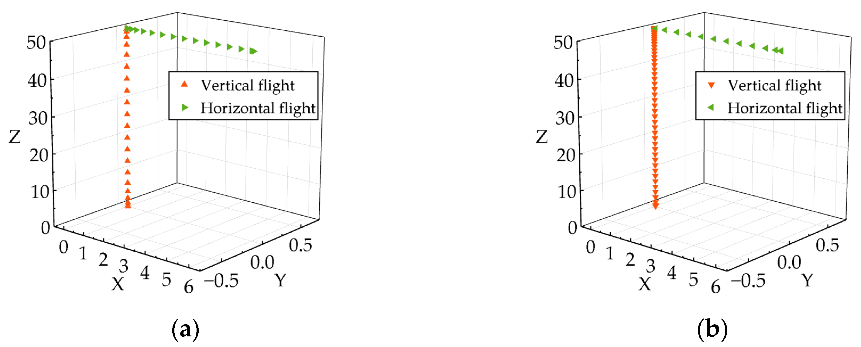
6.2. Flight Mission Path Simulation

The Simulink platform is used to validate flight mission paths, energy consumption, and execution time through simulation tests. Figure 13 shows the simulation model. The model consists of five modules: path command, position controller, attitude controller, rotor motor hybrid controller, and flight dynamics. The path command module converts the input FPTLIR flight path command into the current position; the position control module transforms the current position of the FPTLIR into an attitude control command; the attitude control module employs a traditional PID control algorithm to control the attitude of the FPTLIR; the rotor motor hybrid control module decodes the output of the attitude control module into individual rotor motor control commands; and finally, the flight dynamics module includes a dynamic model representing the FPTLIR’s behavior during flight as discussed in the previous sections. The simulation model uses the optimized path parameters, which are obtained from the improved speed curve, to generate the corresponding task path and energy consumption–time curves.

The flight mission paths of the FPTLIR for the on-line and off-line missions are shown in Figure 14a and Figure 14b, respectively, in the inertial reference system. The simulation model generates corresponding 3D trajectories by recording trajectory points at 0.5 s intervals, thereby representing the magnitude of velocity through the density of trajectory points. Initially, the FPTLIR hovers at Point (#1) with coordinates (0,0,0), then rises vertically to reach Point (#2) with coordinates (0,0,49.9058). It then transitions to horizontal forward flight and finally arrives at Point (#3) with coordinates (5.9655,0,49.9058). The FPTLIR then performs a horizontal backward flight from Point (#4) with coordinates (6.0000,0,50.0000) to Point (#5) with coordinates (0.0361,0,50.0000), before finally reaching its destination at Point (#6) with coordinates (0.0361,0,0.0764). The results show that the FPTLIR effectively responds to input commands and successfully completes flight missions while meeting stability, safety, positional accuracy, and other relevant indicators and constraints.

Correspondingly, Figure 15a,b depict the energy consumption profiles of the optimized flight during on-line and off-line simulations, respectively. The results indicate that the FPTLIR completes the on-line mission in a total time of 17.81 s with a corresponding energy consumption of 1.3188 × 10⁵ J. Compared to the actual numerical calculations, we observe a time error of only 0.22% and an energy consumption error of only 1.31%. Similarly, for the off-line mission, the FPTLIR achieves it within a total time of 28.92 s while consuming approximately 1.2735 × 10⁵ J of energy, resulting in negligible errors compared to the actual numerical calculations (time error: 0.49%, energy consumption error: 0.19%). The proposed energy model and optimization method demonstrate consistency and accuracy in predicting and optimizing the energy consumption and mission execution time of the FPTLIR during a mission, closely matching the actual observations.

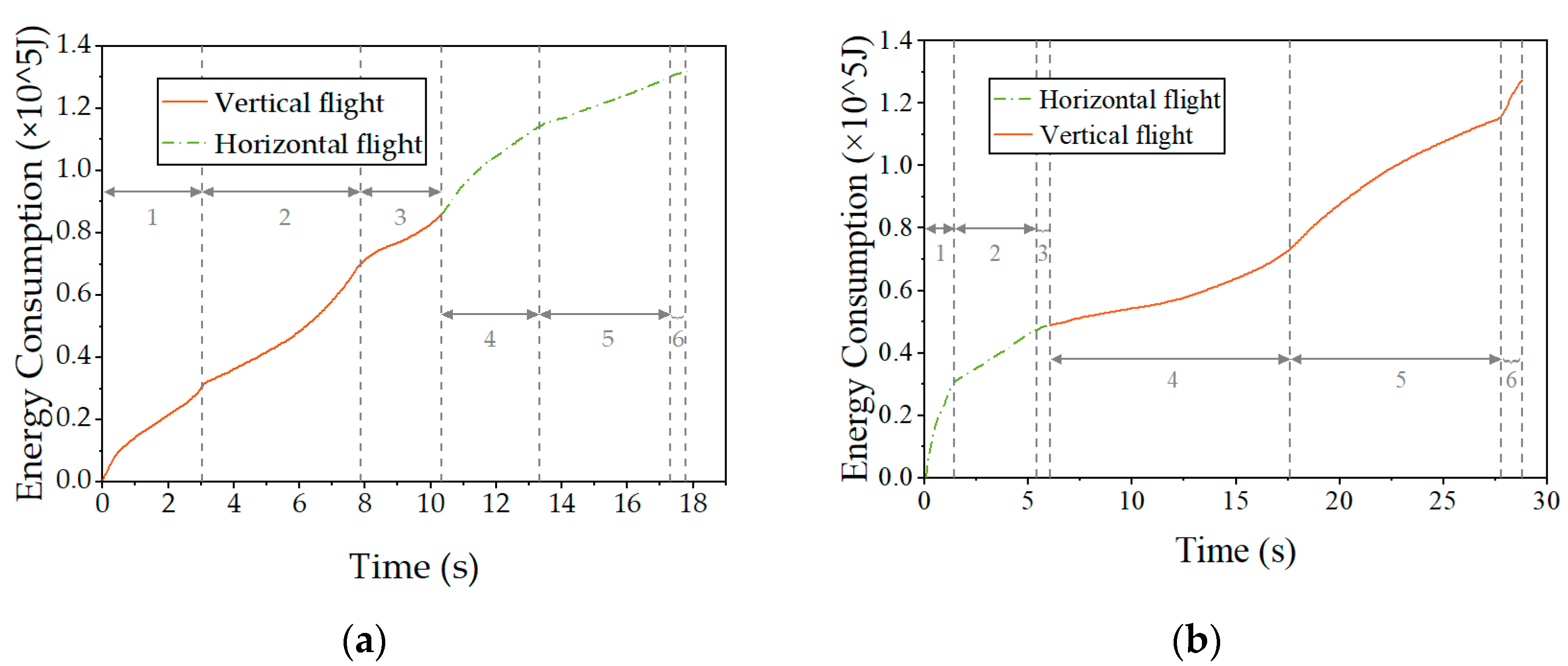
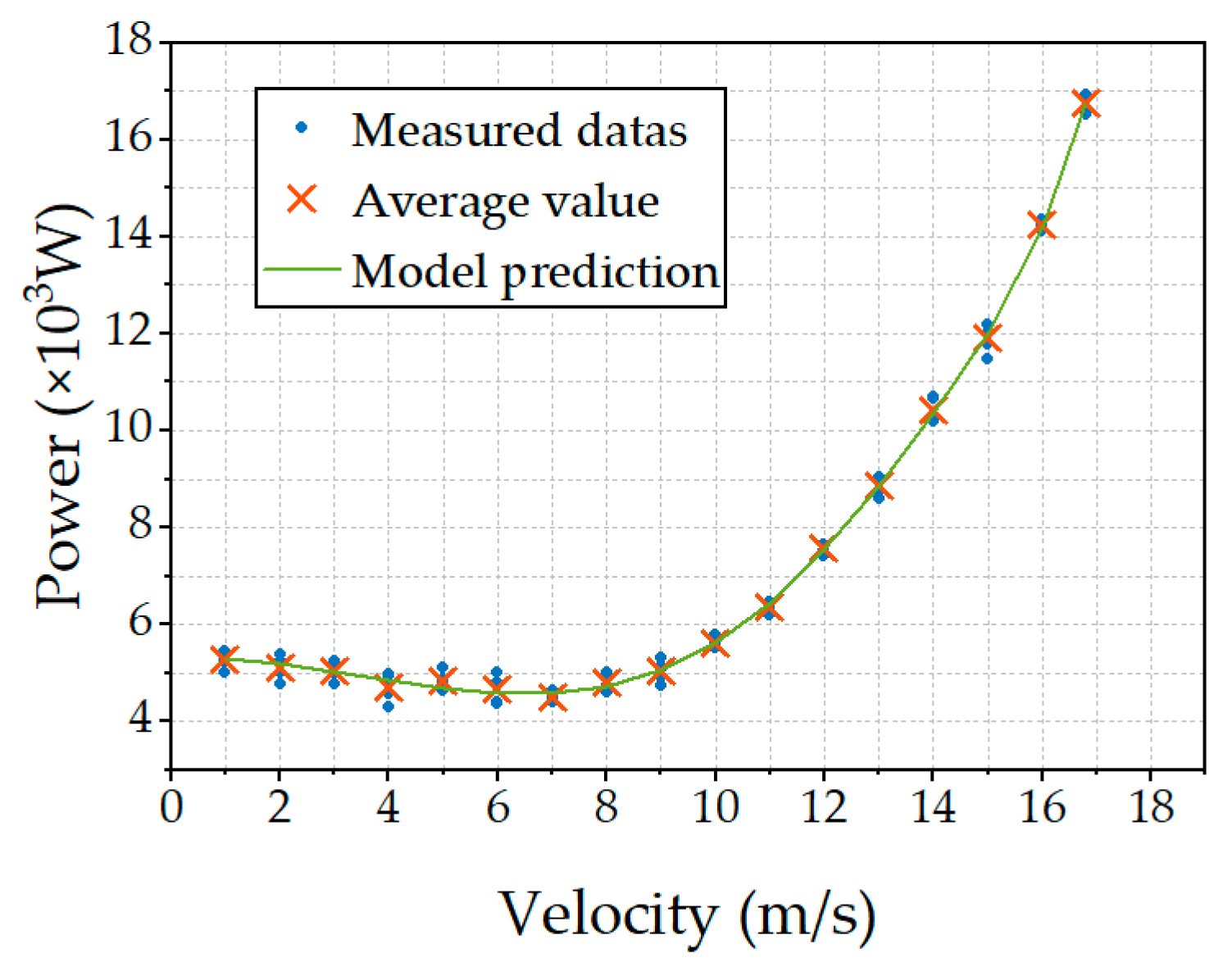
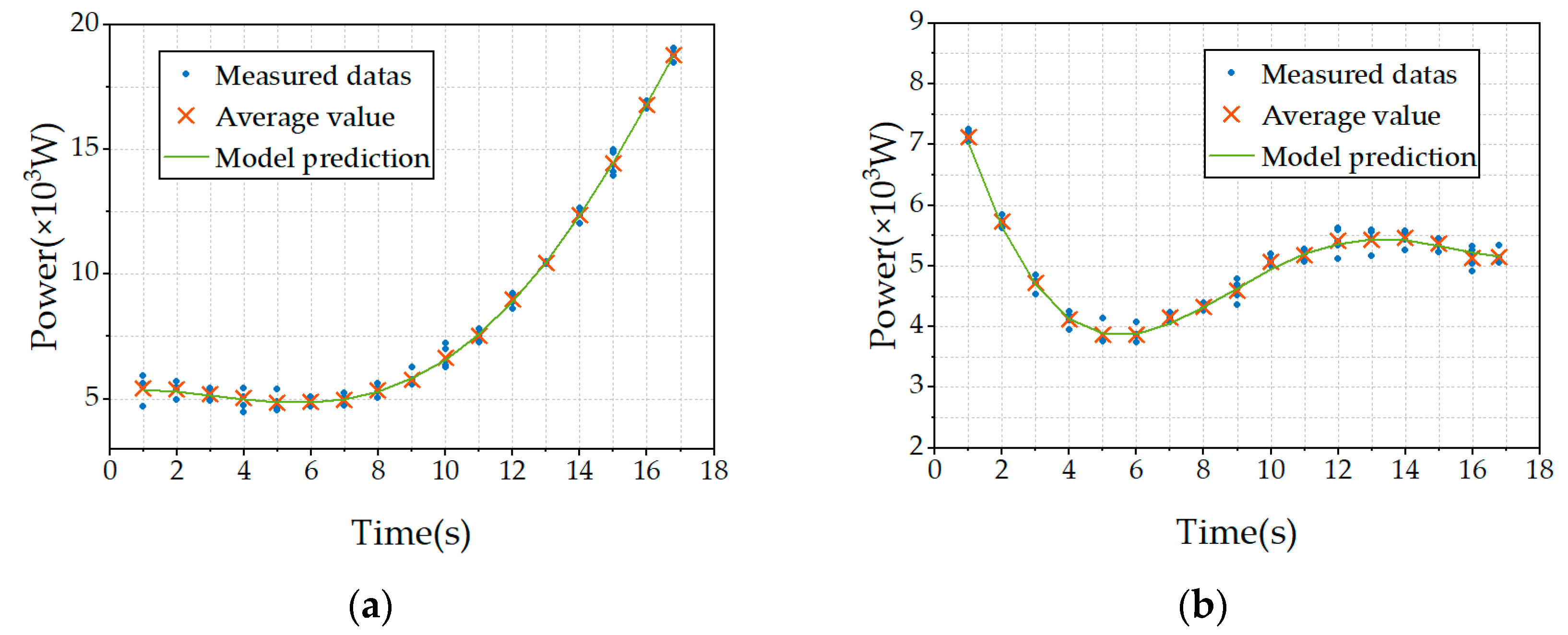
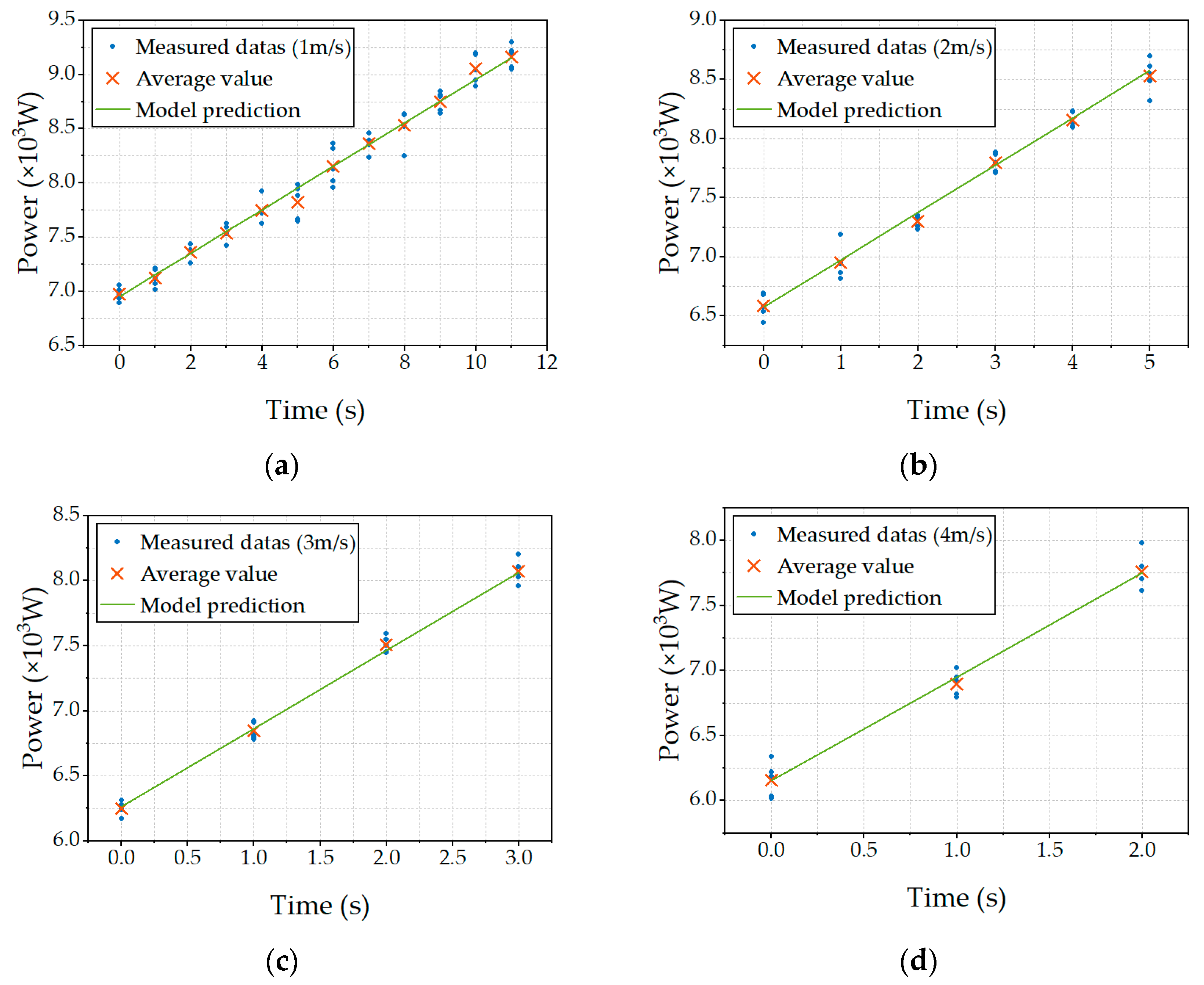
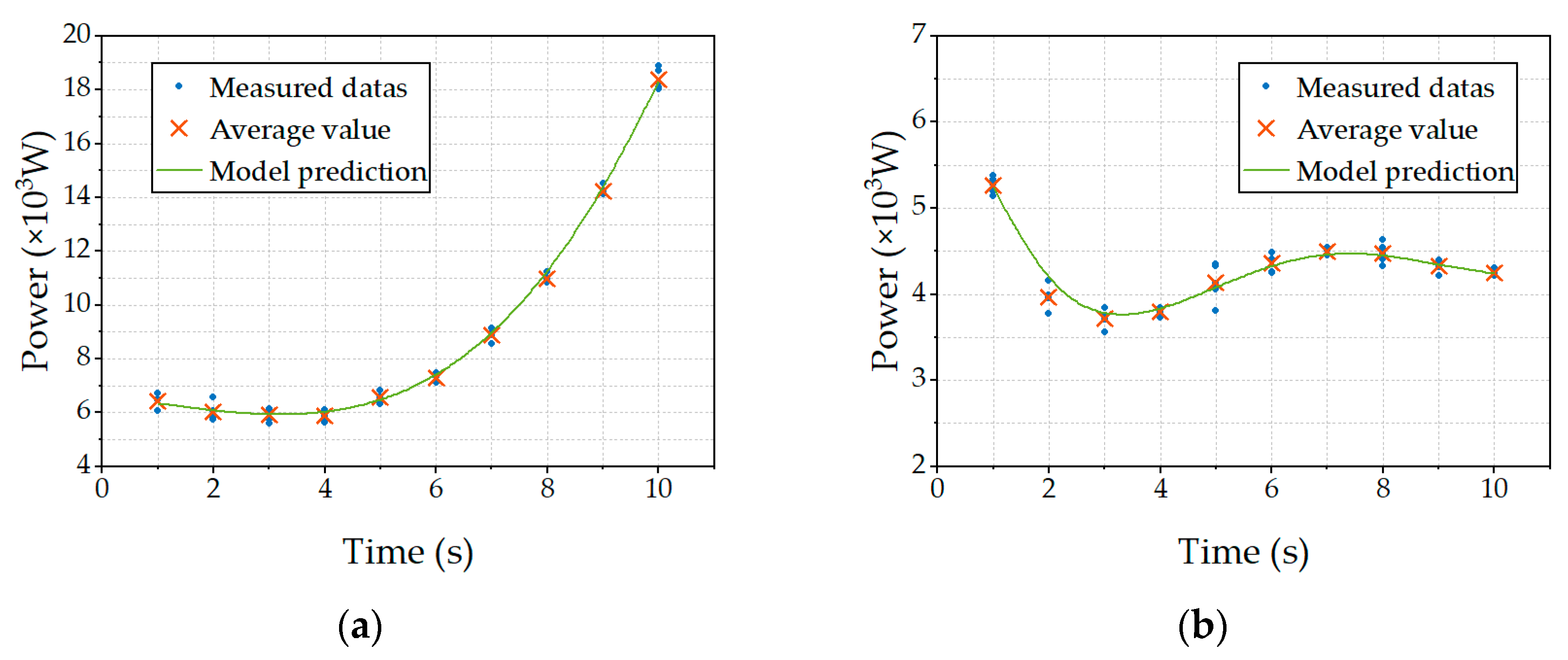
6.3. Energy Consumption Model Validation Tests

To verify the accuracy of the flight system energy consumption model under real flight conditions, a test platform has been independently developed, as shown in Figure 16. The platform is equipped with a Pixhawk 4 flight controller, a current sensor, and a voltage sensor. The current sensor has a measurement error of ±0.9%, while the voltage sensor’s measurement error is mainly due to the voltage divider with a tolerance of 0.1%. Both the current and voltage sensors have a data acquisition frequency of 1 Hz, allowing for one data measurement per second.

Under the control of the Pixhawk 4 flight controller, various flight commands were executed on the FPTLIR to measure, record, and analyze related data using an upper computer interface. Specifically, system power was measured by recording the output current and voltage of the FPTLIR’s battery during static, horizontal, and vertical flight states under the actual route conditions. Experimental data were then compared with model prediction data to verify model accuracy.

As part of the preparatory work prior to line inspections, the flight on-line and off-line missions are usually chosen to be carried out in a relatively stable external environment in order to ensure safety and reliability. When performing the validation tests for the energy consumption model, it is important to simulate the actual outdoor environment during the flight mission as closely as possible. The test site was strategically located between buildings with no obstructions along the flight path to minimize the influence of external factors on the FPTLIR. A constant ambient temperature of 25 °C was maintained throughout the test period. Initially, a static test was performed with a normal communication link between the FPTLIR and the ground computer, with the propeller not turning, resulting in a quiescent system state. In this state, the total power consumption of the FPTLIR remained stable at 29.7 W, including all open components and sensors. Subsequent experimental measurements ignored the power consumption in this static state.

The first flight test involved horizontal constant velocity flights, where FPTLIR flew in straight lines at a fixed altitude of 4 m. Starting from a hovering state at 0 m/s, the velocity was gradually increased in increments of 1 m/s until it reached 16.8 m/s. Each speed level was maintained for 5 s, with data collected every second. Due to site constraints, the tests were completed in batches. Figure 17 shows the instantaneous power measurements at different horizontal speeds and average power values over each 5 s period, together with the corresponding prediction curves based on the energy consumption model of the flight systems. From Figure 17, it can be seen that the power of the FPTLIR shows a decreasing and then increasing trend with increasing speed during horizontal flights at uniform velocities. The average error in predicting the power of the FPTLIR under such conditions is calculated to be approximately 0.1553 × 10³ W with an average relative error rate of approximately 2.56%.

The second flight test consisted of several horizontal forward flights at variable velocities. During the test, the FPTLIR was first accelerated in a straight line at a fixed altitude of 4 m. The speed was gradually increased from 0 m/s (hover) to 16.8 m/s with an acceleration of 1 m/s². The speed was then gradually reduced with a deceleration of 1 m/s². The test was repeated five times. Figure 18a,b shows the instantaneous power measurements during both the acceleration and deceleration phases, as well as the average power values for all five trials and the corresponding prediction curves based on the energy consumption model of the flight systems. For power prediction during the acceleration phase, there is an average error of 0.2114 × 10³ W with an average relative error of 3.24%. For power prediction during the deceleration phase, there is an average error of 0.0988 × 10³ W with an average relative error of 2.03%.

The third flight test involved several vertical constant velocity flights, where the FPTLIR ascended at a steady rate of 1 m/s, 2 m/s, 3 m/s, and 4 m/s within the height range of 4 m to 16 m. Each velocity was repeated five times for testing purposes. Figure 19 shows the instantaneous power measurements at different vertical velocities, together with the average power value obtained from five trials and the corresponding prediction curves based on the energy consumption model of the flight systems. The initial phase from ground level to 4 m altitude served as an acceleration and deceleration stage for ensuring appropriate test velocities and safe landing speeds for the FPTLIR. For power prediction at uniform ascent velocities of 1 m/s, 2 m/s, 3 m/s, and 4 m/s, the average errors are found to be 0.0879 × 10³ W, 0.0831 × 10³ W, 0.0551 × 10³ W, and 0.0971 × 10³ W respectively. The corresponding average relative errors are found to be approximately at levels of 1.08%, 1.11%, 0.76%, and 1.41%.

The fourth flight test involved several vertical variable velocity flights, where the FPTLIR’s velocity was gradually increased from 0 m/s (hovering state) to 10 m/s with an acceleration of 1 m/s². Subsequently, the velocity was gradually reduced with a deceleration of 1 m/s² and repeated for five trials. Figure 20a,b shows the instantaneous power measurements during both the acceleration and deceleration states, together with the average power value obtained from five trials and the corresponding prediction curves based on the energy consumption model of the flight system. For power prediction during acceleration, there is an average error of 0.1914 × 10³ W with an average relative error of 2.43%. Similarly, for power prediction during deceleration, there is an average error of 0.0774 × 10³ W with an average relative error of 1.83%.

The model shows satisfactory performance in predicting the power of the FPTLIR over different flight paths and operational states. It is observed that the model has a higher prediction bias during horizontal flight when compared to vertical flight. This is due to the air disturbance caused by the forward motion and mutual interference of the airflow between the rotors, which affects the accuracy of the momentum theory when applied to horizontal flight.

7. Discussion

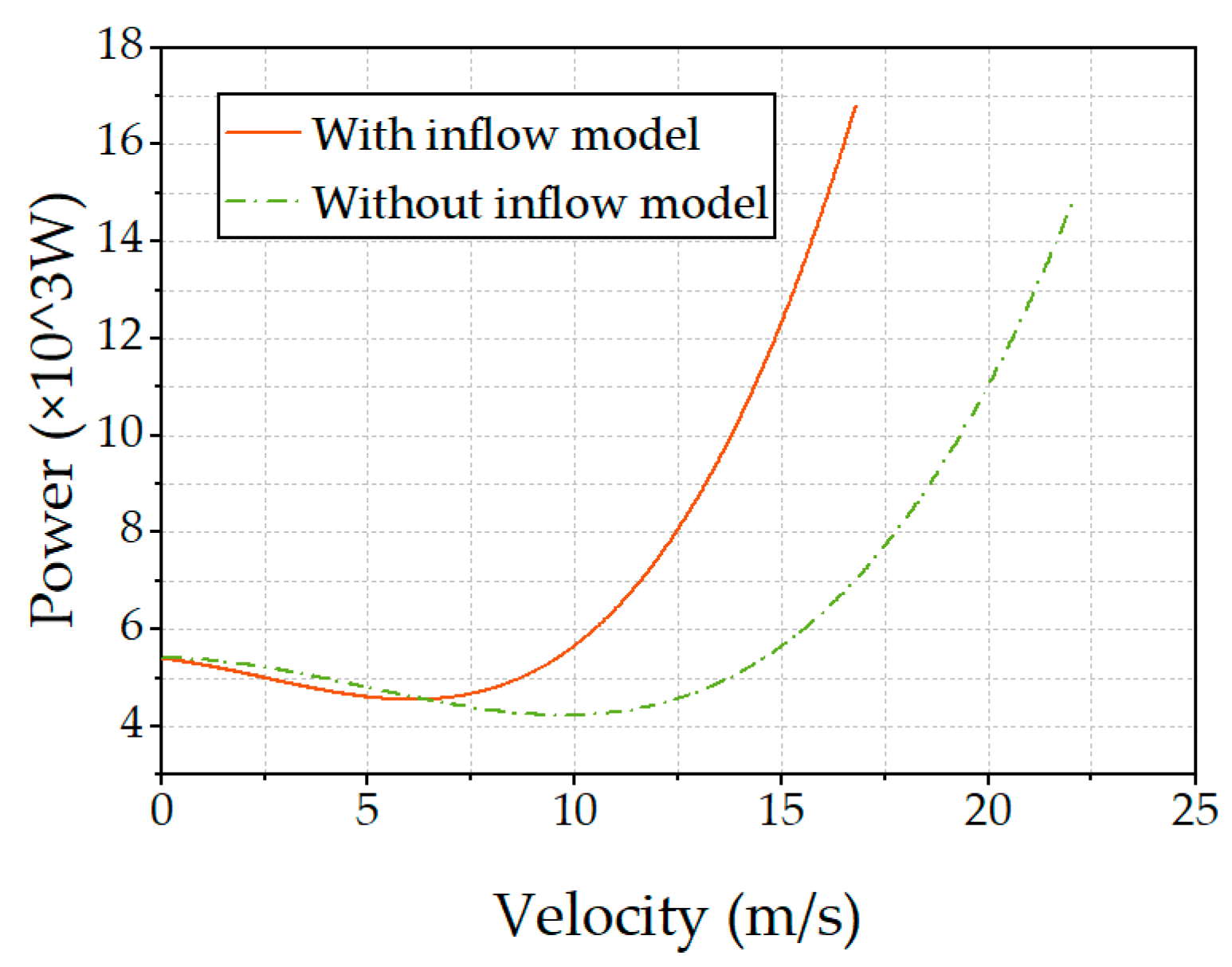
7.1. Effect of the Key Parameters on Energy Modeling

Taking the relationship between horizontal flight velocity and the FPTLIR power as an example, Figure 21 shows a comparison of the full energy model with the simplified model that neglects propeller aerodynamics. From Figure 21, it can be seen that the FPTLIR power does not change monotonically with increasing velocity, but shows an initial decrease followed by an increase. Through analysis, it is observed that several factors contribute to this condition. Firstly, as the flight velocity increases, the power consumption decreases as the incoming velocity perpendicular to the propeller’s plane of rotation increases, resulting in an increase in thrust. This effect is more pronounced at lower FPTLIR velocities. Once the power consumption of the FPTLIR reaches its minimum point, the increase in forward velocity results in a quadratic increase in airframe drag with respect to velocity. This has a negative effect on the FPTLIR performance, particularly at higher velocities, and subsequently results in increased power consumption. As the velocity increases, the pitch angle of the FPTLIR also increases, resulting in an increase in the power required to maintain vertical force equilibrium, again with a greater effect at high velocities. Figure 21 shows that neglecting propeller aerodynamics results in significant errors in the estimation of the model performance. This leads to an overestimation of energy consumption at low velocities and an underestimation at high velocities. In addition, deviations are observed in both the velocities corresponding to minimum FPTLIR power and maximum achievable velocities. As the application of the FPTLIR in complex natural environments continues to expand, it is particularly important to analyze in depth the effects of aerodynamic and environmental factors (especially wind) on its energy consumption and flight dynamics. Future research will analyze the FPTLIR in more complex environments, which will improve the applicability and accuracy of the model.

7.2. Comparison of Different Algorithms

To validate the superiority of the improved NSGA-II algorithm in solving the FPTLIR mission path energy–time optimization problem, a series of experiments was conducted using the improved NSGA-II algorithm, the standard NSGA-II algorithm, and the MOPSO algorithm to primarily compare their convergence, coverage, solution diversity, and computational efficiency. All algorithms were implemented in MATLAB with consistent basic parameter settings and runtime environment on a computer equipped with an Intel (R) Core (TM) i5-7300HQ processor. During the experiment, each optimization algorithm was executed multiple times to calculate average values for relevant performance metrics. Common metrics such as Generational Distance (GD), which measures the distance between solutions generated by the algorithm and the true Pareto front, are used to assess convergence; the mean Hypervolume (HV), which considers both the distance and volume between solutions in the frontier, serves as a metric for characterizing coverage of the Pareto frontier; the size of the Pareto frontier indicates the number of solutions within it and demonstrates solution diversity; runtime is used to measure computational efficiency. The performance metrics at different iterations are listed in

Table 5. The performance metrics at different iterations.

	Iterations	1	10	20	30	40	50
Algorithm/Parameter
Improved NSGA-II	GD	0.131	0.042	0.018	0.006	0.007	0.004
	Mean HV	0.542	0.727	0.784	0.899	0.972	0.989
	Pareto front size	35	44	49	52	50	50
	Running time (s)	0.846	4.225	7.624	12.342	17.563	22.364
Standard NSGA-II	GD	0.216	0.124	0.101	0.086	0.057	0.036
	Mean HV	0.421	0.542	0.692	0.684	0.724	0.821
	Pareto front size	21	33	42	39	41	45
	Running time (s)	0.692	3.964	6.017	8.117	12.031	16.247
MOPSO	GD	0.203	0.152	0.128	0.093	0.059	0.057
	Mean HV	0.433	0.494	0.511	0.753	0.724	0.805
	Pareto front size	22	29	36	43	41	43
	Running time (s)	0.765	3.721	5.924	8.214	11.220	15.434

.

Comparing the results in Table 5, it can be seen that the improved NSGA-II algorithm has a lower GD value compared to both the standard NSGA-II algorithm and the MOPSO algorithm, indicating better convergence accuracy. Furthermore, based on the higher mean HV and Pareto front size values, it can be seen that the improved NSGA-II algorithm has a better uniformity and distribution quality of solutions in the objective space. Consequently, it is more suitable for multiobjective optimization problems with complex constraints, such as those presented in this paper. The comparison of running time shows that the improved NSGA-II algorithm requires a longer running time for the same number of iterations due to the increased complexity. However, despite this longer duration, its significant advantages compensate for this additional time cost when solving the complex multiobjective optimization problems discussed here. A comprehensive analysis of these results leads to the conclusion that the improved NSGA-II algorithm is not optimal in all cases, but it shows significant advantages when dealing with the complex multiobjective optimization problems discussed in this paper.

7.3. Limitations and Future Work

The voltage of the battery supplying power to the FPTLIR gradually decreases during mission execution, resulting in consequential variations in its performance and subsequent impact on energy consumption. This paper primarily focuses on modeling the energy demand side of the FPTLIR during mission paths; however, it does not fully consider the influence of battery voltage variations. Therefore, future studies should include variations in battery-related parameters to better understand their impact on the FPTLIR energy consumption.

In addition, considering the complexity of multiobjective optimization models based on flight energy models, we chose to study only the simplest sequence of flight state transition times when dividing path intervals by flight states. However, the precision with which state intervals are partitioned has a significant effect on optimization effectiveness and speed. As the partitioning accuracy increases, optimization effectiveness improves but at the cost of increased optimization time. In future research, these two effects should be comprehensively considered to moderately improve the precision of state interval partitioning to better optimize the FPTLIR energy consumption.

The computational efficiency of algorithms is also crucial for real-time application scenarios. In particular, for real-world applications that require rapid response and decision making, the complexity of the algorithm and the time required for optimization become factors that cannot be ignored. With this in mind, future research will focus on deploying the methods in this paper in real-time application scenarios and improving the computational efficiency of the NSGA-II algorithm to meet the demands of practical applications. In addition, given the specificity and complexity of transmission line inspection, exploration of algorithm customization for specific application scenarios will be pursued to ensure more efficient and accurate optimization results, thereby providing a more effective and reliable technical solution in the field of transmission line inspection.

8. Conclusions

In this paper, a multiobjective optimization approach is proposed using the improved NSGA-II algorithm. This approach considers various constraints and flight states during the FPTLIR flight missions, using the derived energy consumption model as the objective function. The main objective is to minimize the energy consumption of the system and ensure the shortest mission execution time under corresponding energy consumption, while satisfying the constraints.

• A mathematical model of system-level energy consumption was derived. The relationship between the mission path and energy consumption of the FPTLIR was established by progressively deriving from the FPTLIR kinematics to end-effector motor dynamics, making the model more suitable for constructing the multiobjective optimization model. The incorporation of the blade unit theory and aerodynamic analysis improved the accuracy of the energy consumption model. The prediction accuracy of the energy consumption model is further improved by using a self-built test platform to measure and fit the energy consumption model parameters. After experimental validation in different paths and flight states, the model showed good performance with an average relative error ranging from 0.76% to 3.24% compared to actual power predictions;
• A multiobjective optimization model was constructed based on the energy consumption model, considering energy consumption and execution time under the flight mission path. The adaptability to real mission requirements was improved by quantifying the stability, safety, and other relevant constraints of the FPTLIR during mission execution, along with integrating the analysis of energy consumption in complex flight states;
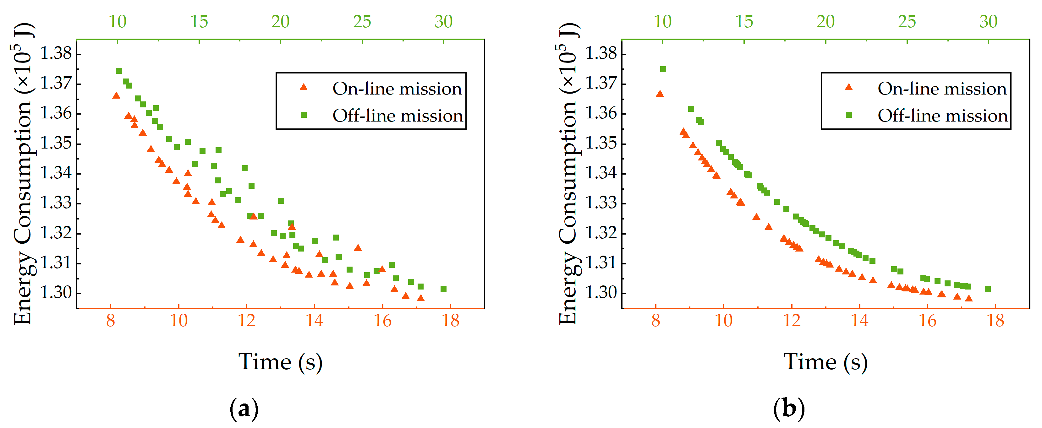
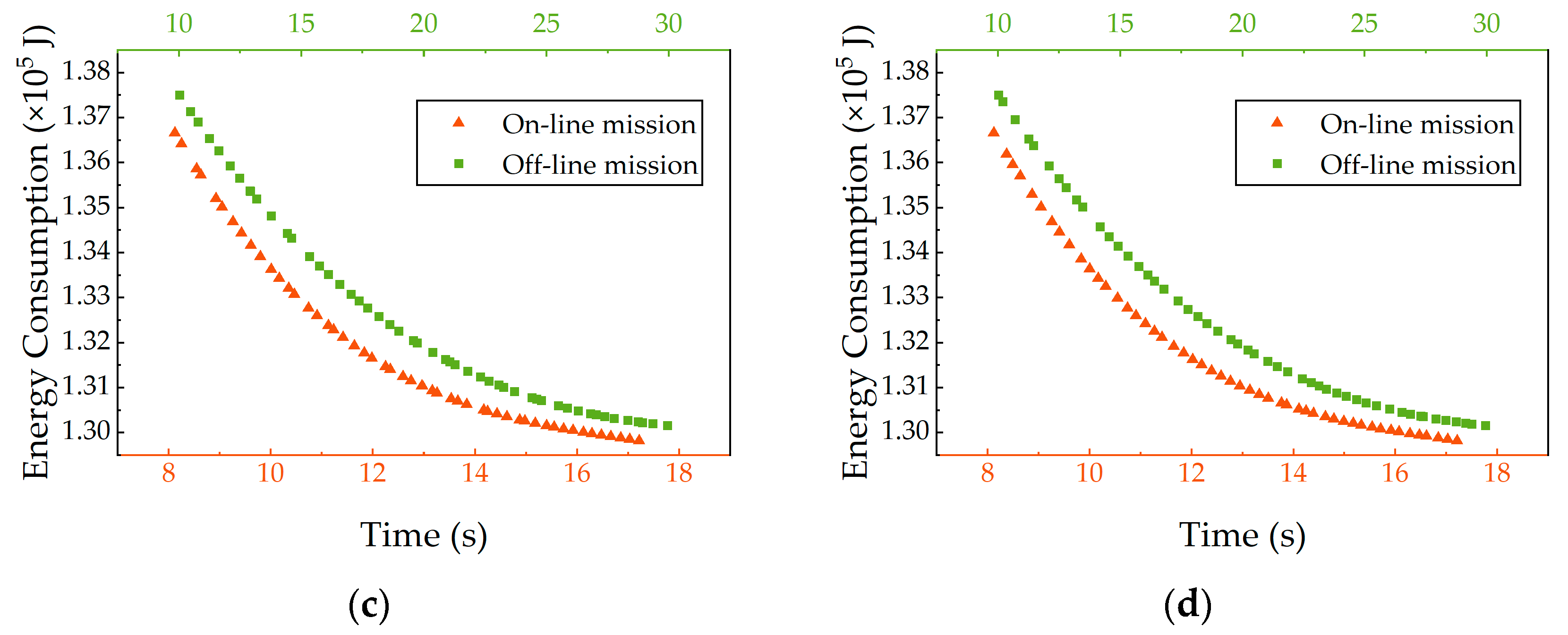
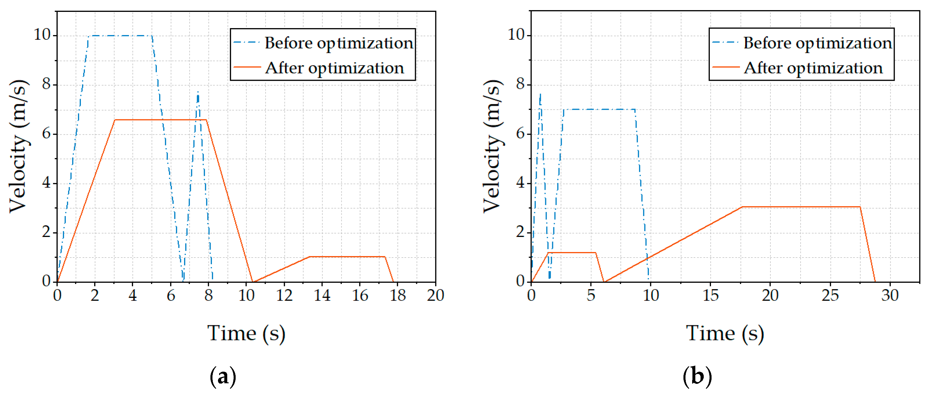
• An optimization approach based on the improved NSGA-II algorithm was proposed to optimize the energy consumption and mission execution time of the FPTLIR during flight missions. The NSGA-II optimization algorithm was improved by incorporating the Cauchy variation operator and integrating the principles of simulated annealing, thereby improving its robustness and local search capability in complex constraint scenarios. The optimal energy consumption for completing the on-line mission in the shortest time of 8.22 s was determined as 1.3750 × 10⁵ J. Following optimization, the shortest total time for completing the on-line mission with the lowest energy consumption of 1.3017 × 10⁵ J was determined as 17.77 s, saving 5.33% of energy consumption. Similarly, for completing off-line missions within a minimal timeframe of 9.84 s, the optimal energy consumption was found to be 1.3667 × 10⁵ J. After optimization, the shortest time for completing the off-line mission was 28.78 s with the minimum energy consumption of 1.2983 × 10⁵ J, saving 5.01% of energy consumption. The proposed optimization approach effectively minimized energy consumption while ensuring minimal mission execution times at corresponding energy consumption levels, thereby improving the overall system flight efficiency.

References

1. Hu, Y.; Wen, B.; Ye, Y.; Yang, C. Multi-Defect Detection Network for High-Voltage Insulators Based on Adaptive Multi-Attention Fusion. Appl. Sci. 2023, 13, 13351. [Google Scholar] [CrossRef]
2. Yang, L.; Fan, J.; Liu, Y.; Li, E.; Peng, J.; Liang, Z. A Review on State-of-the-Art Power Line Inspection Techniques. IEEE Trans. Instrum. Meas. 2020, 69, 9350–9365. [Google Scholar] [CrossRef]
3. Menendez, O.; Auat Cheein, F.A.; Perez, M.; Kouro, S. Robotics in Power Systems: Enabling a More Reliable and Safe Grid. IEEE Ind. Electron. Mag. 2017, 11, 22–34. [Google Scholar] [CrossRef]
4. Foudeh, H.A.; Luk, P.; Whidborne, J. Application of Norm Optimal Iterative Learning Control to Quadrotor Unmanned Aerial Vehicle for Monitoring Overhead Power System. Energies 2020, 13, 3223. [Google Scholar] [CrossRef]
5. Cantieri, A.; Ferraz, M.; Szekir, G.; Antônio Teixeira, M.; Lima, J.; Schneider Oliveira, A.; Aurélio Wehrmeister, M. Cooperative UAV–UGV Autonomous Power Pylon Inspection: An Investigation of Cooperative Outdoor Vehicle Positioning Architecture. Sensors 2020, 20, 6384. [Google Scholar] [CrossRef] [PubMed]
6. Guan, H.; Sun, X.; Su, Y.; Hu, T.; Wang, H.; Wang, H.; Peng, C.; Guo, Q. UAV-Lidar Aids Automatic Intelligent Powerline Inspection. Int. J. Electr. Power Energy Syst. 2021, 130, 106987. [Google Scholar] [CrossRef]
7. Liu, Y.; Shi, J.; Liu, Z.; Huang, J.; Zhou, T. Two-Layer Routing for High-Voltage Powerline Inspection by Cooperated Ground Vehicle and Drone. Energies 2019, 12, 1385. [Google Scholar] [CrossRef]
8. Fan, F.; Wu, G.; Wang, M.; Cao, Q.; Yang, S. Multi-Robot Cyber Physical System for Sensing Environmental Variables of Transmission Line. Sensors 2018, 18, 3146. [Google Scholar] [CrossRef]
9. Yue, X.; Feng, Y.; Jiang, B.; Wang, L.; Hou, J. Automatic Obstacle-Crossing Planning for a Transmission Line Inspection Robot Based on Multisensor Fusion. IEEE Access 2022, 10, 63971–63983. [Google Scholar] [CrossRef]
10. Gonçalves, R.S.; Carvalho, J.C.M. A Mobile Robot to Be Applied in High-Voltage Power Lines. J. Braz. Soc. Mech. Sci. Eng. 2015, 37, 349–359. [Google Scholar] [CrossRef]
11. Alhassan, A.B.; Zhang, X.; Shen, H.; Xu, H. Power Transmission Line Inspection Robots: A Review, Trends and Challenges for Future Research. Int. J. Electr. Power Energy Syst. 2020, 118, 105862. [Google Scholar] [CrossRef]
12. Miralles, F.; Hamelin, P.; Lambert, G.; Lavoie, S.; Pouliot, N.; Montfrond, M.; Montambault, S. LineDrone Technology: Landing an Unmanned Aerial Vehicle on a Power Line. In Proceedings of the 2018 IEEE International Conference on Robotics and Automation (ICRA), Brisbane, QLD, Australia, 21–25 May 2018; pp. 6545–6552. [Google Scholar]
13. Wang, H.; Li, E.; Yang, G.; Guo, R. Design of an Inspection Robot System with Hybrid Operation Modes for Power Transmission Lines. In Proceedings of the 2019 IEEE International Conference on Mechatronics and Automation (ICMA), Tianjin, China, 4–7 August 2019; pp. 2571–2576. [Google Scholar]
14. Bian, J.; Hui, X.; Zhao, X.; Tan, M. A Novel Development of Robots with Cooperative Strategy for Long-Term and Close-Proximity Autonomous Transmission-Line Inspection. In Proceedings of the 2019 International Conference on Robotics and Automation (ICRA), Montreal, QC, Canada, 20–24 May 2019; pp. 1898–1904. [Google Scholar]
15. Morbidi, F.; Cano, R.; Lara, D. Minimum-Energy Path Generation for a Quadrotor UAV. In Proceedings of the 2016 IEEE International Conference on Robotics and Automation (ICRA), Stockholm, Sweden, 16–21 May 2016; pp. 1492–1498. [Google Scholar]
16. Chang, W.; Yang, G.; Yu, J.; Liang, Z.; Cheng, L.; Zhou, C. Development of a Power Line Inspection Robot with Hybrid Operation Modes. In Proceedings of the 2017 IEEE/RSJ International Conference on Intelligent Robots and Systems (IROS), Vancouver, BC, Canada, 24–28 September 2017; pp. 973–978. [Google Scholar]
17. Li, Z.; Tian, Y.; Yang, G.; Li, E.; Zhang, Y.; Chen, M.; Liang, Z.; Tan, M. Vision-Based Autonomous Landing of a Hybrid Robot on a Powerline. IEEE Trans. Instrum. Meas. 2023, 72, 3501711. [Google Scholar] [CrossRef]
18. Shen, H.; Zhang, X.; Alhassan, A.B.; Xu, H.; Zhang, X.; Huang, W. Research on the Adaptive Control Method of Pre-Landing for High Voltage Transmission Line Inspection Robot Based on Multi-Body Transfer Matrix Method. In Proceedings of the 2020 10th Institute of Electrical and Electronics Engineers International Conference on Cyber Technology in Automation, Control, and Intelligent Systems (CYBER), Xi’an, China, 10–14 October 10 2020; pp. 312–317. [Google Scholar]
19. Zhang, T.; Dai, J. Electric Power Intelligent Inspection Robot: A Review. J. Phys. Conf. Ser. 2021, 1750, 012023. [Google Scholar] [CrossRef]
20. Yang, Z.; Xu, W.; Shikh-Bahaei, M. Energy Efficient UAV Communication with Energy Harvesting. IEEE Trans. Veh. Technol. 2020, 69, 1913–1927. [Google Scholar] [CrossRef]
21. Zeng, Y.; Zhang, R. Energy-Efficient UAV Communication with Trajectory Optimization. IEEE Trans. Wirel. Commun. 2017, 16, 3747–3760. [Google Scholar] [CrossRef]
22. Beigi, P.; Rajabi, M.S.; Aghakhani, S. An Overview of Drone Energy Consumption Factors and Models; Springer: Geneva, Switzerland, 2022. [Google Scholar]
23. Jia, G.; Li, C.; Li, M. Energy-Efficient Trajectory Planning for Smart Sensing in IoT Networks Using Quadrotor UAVs. Sensors 2022, 22, 8729. [Google Scholar] [CrossRef] [PubMed]
24. Hong, D.; Lee, S.; Cho, Y.H.; Baek, D.; Kim, J.; Chang, N. Least-Energy Path Planning with Building Accurate Power Consumption Model of Rotary Unmanned Aerial Vehicle. IEEE Trans. Veh. Technol. 2020, 69, 14803–14817. [Google Scholar] [CrossRef]
25. Wu, M.; Chen, W.; Tian, X. Optimal Energy Consumption Path Planning for Quadrotor UAV Transmission Tower Inspection Based on Simulated Annealing Algorithm. Energies 2022, 15, 8036. [Google Scholar] [CrossRef]
26. Góra, K.; Smyczyński, P.; Kujawiński, M.; Granosik, G. Machine Learning in Creating Energy Consumption Model for UAV. Energies 2022, 15, 6810. [Google Scholar] [CrossRef]
27. Abeywickrama, H.V.; Jayawickrama, B.A.; He, Y.; Dutkiewicz, E. Comprehensive Energy Consumption Model for Unmanned Aerial Vehicles, Based on Empirical Studies of Battery Performance. IEEE Access 2018, 6, 58383–58394. [Google Scholar] [CrossRef]
28. Prasetia, A.S.; Wai, R.-J.; Wen, Y.-L.; Wang, Y.-K. Mission-Based Energy Consumption Prediction of Multirotor UAV. IEEE Access 2019, 7, 33055–33063. [Google Scholar] [CrossRef]
29. Yacef, F.; Rizoug, N.; Degaa, L.; Bouhali, O.; Hamerlain, M. Energy Efficiency Path Planning for a Quadrotor Aerial Vehicle. Trans. Inst. Meas. Control 2021, 014233122110585. [Google Scholar] [CrossRef]
30. Dai, X.; Duo, B.; Yuan, X.; Tang, W. Energy-Efficient UAV Communications: A Generalized Propulsion Energy Consumption Model. IEEE Wirel. Commun. Lett. 2022, 11, 2150–2154. [Google Scholar] [CrossRef]
31. Yan, H.; Chen, Y.; Yang, S.-H. New Energy Consumption Model for Rotary-Wing UAV Propulsion. IEEE Wirel. Commun. Lett. 2021, 10, 2009–2012. [Google Scholar] [CrossRef]
32. Li, B.; Na, Z.; Lin, B. UAV Trajectory Planning from a Comprehensive Energy Efficiency Perspective in Harsh Environments. IEEE Netw. 2022, 36, 62–68. [Google Scholar] [CrossRef]
33. Na, Y.; Li, Y.; Chen, D.; Yao, Y.; Li, T.; Liu, H.; Wang, K. Optimal Energy Consumption Path Planning for Unmanned Aerial Vehicles Based on Improved Particle Swarm Optimization. Sustainability 2023, 15, 12101. [Google Scholar] [CrossRef]
34. Gao, H.; Lee, W.; Li, W.; Han, Z.; Osher, S.; Poor, H.V. Energy-Efficient Velocity Control for Massive Numbers of Rotary-Wing UAVs: A Mean Field Game Approach. In Proceedings of the GLOBECOM 2020—2020 IEEE Global Communications Conference, Taipei, Taiwan, 7–11 December 2020; pp. 1–6. [Google Scholar]
35. Yazdinejad, A.; Dehghantanha, A.; Parizi, R.M.; Epiphaniou, G. An Optimized Fuzzy Deep Learning Model for Data Classification Based on NSGA-II. Neurocomputing 2023, 522, 116–128. [Google Scholar] [CrossRef]
36. Yazdinejad, A.; Parizi, R.M.; Dehghantanha, A.; Srivastava, G.; Mohan, S.; Rababah, A.M. Cost Optimization of Secure Routing with Untrusted Devices in Software Defined Networking. J. Parallel Distrib. Comput. 2020, 143, 36–46. [Google Scholar] [CrossRef]
37. Yazdinejad, A.; Parizi, R.M.; Dehghantanha, A.; Karimipour, H.; Srivastava, G.; Aledhari, M. Enabling Drones in the Internet of Things with Decentralized Blockchain-Based Security. IEEE Internet Things J. 2021, 8, 6406–6415. [Google Scholar] [CrossRef]
38. Yazdinejad, A.; Parizi, R.M.; Dehghantanha, A.; Karimipour, H. Federated Learning for Drone Authentication. Ad Hoc Netw. 2021, 120, 102574. [Google Scholar] [CrossRef]
39. Zhang, J.; Lei, J.; Qin, X.; Li, B.; Li, Z.; Li, H.; Zeng, Y.; Song, J. A Fitting Recognition Approach Combining Depth-Attention YOLOv5 and Prior Synthetic Dataset. Appl. Sci. 2022, 12, 11122. [Google Scholar] [CrossRef]
40. Johnson, W. Helicopter Theory; Courier Corporation: Chelmsford, MA, USA, 2012; ISBN 0-486-13182-3. [Google Scholar]
41. Lawrence, D.; Mohseni, K. Efficiency Analysis for Long Duration Electric MAVs. In Proceedings of the Infotech@Aerospace, Arlington, VA, USA, 26–29 September 2005. [Google Scholar]
42. Lundström, D.; Amadori, K.; Krus, P. Validation of Models for Small Scale Electric Propulsion Systems. In Proceedings of the 48th AIAA Aerospace Sciences Meeting Including the New Horizons Forum and Aerospace Exposition, Orlando, FL, USA, 4–7 January 2010. [Google Scholar]
43. Li, H.; Zhang, Q. Multiobjective Optimization Problems with Complicated Pareto Sets, MOEA/D and NSGA-II. IEEE Trans. Evol. Comput. 2009, 13, 284–302. [Google Scholar] [CrossRef]
44. Verma, S.; Pant, M.; Snasel, V. A Comprehensive Review on NSGA-II for Multi-Objective Combinatorial Optimization Problems. IEEE Access 2021, 9, 57757–57791. [Google Scholar] [CrossRef]
45. Orosz, T.; Rassõlkin, A.; Kallaste, A.; Arsénio, P.; Pánek, D.; Kaska, J.; Karban, P. Robust Design Optimization and Emerging Technologies for Electrical Machines: Challenges and Open Problems. Appl. Sci. 2020, 10, 6653. [Google Scholar] [CrossRef]
Figure 1. Schematic diagram of FPTLIR structure: (a) complete machine structure; (b) flight mechanism; (c) travelling mechanism.
Applsci 14 01637 g001
Figure 2. Schematic diagram of FPTLIR system.
Applsci 14 01637 g002
Figure 3. The mission paths of FPTLIR.
Applsci 14 01637 g003
Figure 4. Schematic diagram of system dynamics model.
Applsci 14 01637 g004
Figure 5. Integrated system energy consumption model block diagram.
Applsci 14 01637 g005
Figure 6. Flight path diagram based on space–time network.
Applsci 14 01637 g006
Figure 7. Space–time state network diagram considering FPTLIR’s flight velocity curve.
Applsci 14 01637 g007
Figure 8. Flowchart of the FPTLIR multiobjective optimization algorithm based on improved NSGA-II.
Applsci 14 01637 g008
Figure 9. Optimization results of the improved NSGA-II algorithm with different algebras: (a) the 1st generation; (b) the 10th generation; (c) the 30th generation; (d) the 50th generation.
Applsci 14 01637 g009aApplsci 14 01637 g009b
Figure 10. Comparison of velocity curves before and after optimization. (a) Flight on-line mission interval; (b) flight off-line mission interval.
Applsci 14 01637 g010
Figure 11. Test platform for parameter determination of flight system energy consumption model: (1) motor, rotor blade, and internal electronic governor 80A-FOC; (2) parallel beam force sensor; (3) non-contact tachometer; (4) force transmission module; (5) RS485 communication protocol to USB module; (6) STM32 control board; (7) voltage and current detector; (8) voltage and current detector bluetooth transmitter; (9) transformer module; (10) 6S battery (11) 12S battery; (12) direct current (DC) regulated power supply; (13) upper computer.
Applsci 14 01637 g011
Figure 12. Collection data of the test platform. (a) Rotor motor with load test bench data diagram; (b) test bench data diagram of rotor motor without load.
Applsci 14 01637 g012
Figure 13. The simulation model of FPTLIR.
Applsci 14 01637 g013
Figure 14. Flight mission paths of simulation results. (a) Flight on-line mission path; (b) flight off-line mission path.
Applsci 14 01637 g014
Figure 15. Flight energy consumption curve of simulation results. (a) Flight on-line energy consumption curve (123 and 456 are acceleration, uniform, and deceleration stages of vertical and horizontal flights); (b) Flight off-line energy consumption curve (123 and 456 are the acceleration, uniform, and deceleration stages of horizontal and vertical flights, respectively).
Applsci 14 01637 g015
Figure 16. Schematic diagram of the test sites and test equipment. (a) Test sites; (b) flying–walking power transmission line inspection robot; (c) upper computer.
Applsci 14 01637 g016
Figure 17. The power of FPTLIR flying at different constant velocities horizontally.
Applsci 14 01637 g017
Figure 18. The power of FPTLIR flying at uniform variable velocity horizontally. (a) At uniform acceleration; (b) at uniform deceleration.
Applsci 14 01637 g018
Figure 19. The power of FPTLIR flying at different constant velocities vertically. (a) 1 m/s; (b) 2 m/s; (c) 3 m/s; (d) 4 m/s.
Applsci 14 01637 g019
Figure 20. The power of FPTLIR flying at uniform variable velocity vertically. (a) At uniform acceleration; (b) at uniform deceleration.
Applsci 14 01637 g020
Figure 21. Relationship between power and forward velocities.
Applsci 14 01637 g021