Abstract
The current time-domain solution methods for the wavefield equations of a single medium do not apply to the wavefield equations of shallow water seismic with a fluid–elastomer coupling. To solve this problem, based on the explicit central difference method and implicit Newmark method, the explicit–explicit method, implicit–implicit method, and explicit–implicit method time-domain expressions for the local solution are derived, and the time-domain expressions for the explicit and implicit methods in the global solution are derived.The stability and computational efficiency of different time-domain solving methods for the shallow water seismic wavefield equations are theoretically analyzed. The numerical results are compared with the simulation data from the multiphysics field simulation software COMSOL 6.0, and the numerical stability, computational efficiency and accuracy of the different solving methods are also analyzed theoretically. The results show that the implicit method in the global solution is relatively optimal among the methods proposed in this paper, which ensures numerical stability at the larger step size for improving the computational efficiency and considers the higher computational efficiency and accuracy.
1. Introduction
In the shallow water, the vibrations and radiated noises of sailing ships propagate to the seafloor through seawater, stimulating seismic waves. Since undersea seismic waves carry useful target information as a complement to sound waves in water, they have attracted much attention in recent years in underwater target check detection [1,2], target identification [3], and acoustic fuzing of mines [4]. However, submarine seismic wave tests require a lot of human and material resources, so the numerical prediction of the shallow submarine seismic wave field has become an effective way to study its characteristics [5,6]. The high-precision and high-efficiency submarine seismic wave field prediction is of great significance for the application of research on submarine seismic waves.
Acquiring shallow seafloor seismic wavefields requires the time-domain solution of the wavefield equation. Currently, scholars mainly focus on the time-domain solution methods for the single fluid or elastomer fluctuation equation. However, the submarine seismic wavefield equation is obtained by coupling the fluid acoustic pressure fluctuation equation and the elastomer displacement equation, which introduces a coupling term compared with the single equation. Therefore, the single equation solution method is not fully applicable to the solution of the coupled equations. For a single fluid fluctuation equation or elastomer fluctuation equation, both system equations can be expressed by the system mass matrix and stiffness matrix without considering damping, and the only difference lies in the field variables to be solved, which are generally the sound pressure for the fluid fluctuation equation and the displacement for the elastomer fluctuation equation. The classical methods for solving the system equations include the explicit center difference method and the implicit Newmark method [7], based on which scholars have conducted a series of research studies. For the fluid problem, Zhu Changyun [8] and others compared the performance of the explicit central difference method and the implicit Newmark method for the two-dimensional fluctuation equations with a simple example. The results show that the stability of the implicit Newmark method is better than that of the explicit method. However, the accuracy of the explicit method is higher than that of the Newmark method within the stabilization step of the explicit method, and the analysis is not convincing and representative in the simulation of ocean acoustic waves because the example is too simple. Zampieri et al. [9] combined the explicit Newmark method with the isogeometric discretization method for acoustic wave problems with absorbing boundary conditions and analyzed the stability of the method. Although the accuracy and efficiency of the method are better than the finite difference method and the finite element method in some structural acoustics and wave propagation studies, the isogeometric discretization method is severely limited by the size of the discretized mesh and the interpolating polynomial order, which need to be simulated several times to choose the appropriate values. In addition, how to configure the parameters of the isogeometric discretization method is yet to be researched for the elastic wave problems similar to the shallow water seismic waves. For the elastomer problem, Zhou [10] and others proposed a weighted velocity Newmark method to suppress the pseudo-oscillation phenomenon in the dynamic structural rupture problem. However, the selection of the weights is not sufficiently theoretical supported. Yi Ji [11] and others proposed a bisecting step generalized central difference method for general dynamics problems, but it is complicated to solve the relevant parameters for multiple degrees of freedom. The time step is divided into two steps, greatly increasing the computational volume. For the fluid–elastomer coupling problem, Zhaolong [12] and others, based on the theory of saturated porous media, the fluid and elastic solid equilibrium equations decoupled into a single medium equilibrium equation of motion. They used explicit methods to solve the equations and achieve a large-scale simulation of ground vibration of the sea, but the text does not give a specific formula for solving the problem, and the essence of the equation for a single medium is also the solution of the equations. The coupled fluid–elastomer problem is widely studied in the fields of dam protection [13], prediction of ground cracks [14], marine physical exploration [15], and so on. However, scholars have not given specific time-domain solution formulas, and most of the attention is paid to the displacement field in the elastomer.
The methods for obtaining the time-domain submarine seismic wave field induced by acoustic sources in shallow water include experimental methods and numerical simulations. Because of the high cost of experiments for acquiring submarine seismic waves induced by acoustic sources in shallow water, the difficulty of their implementation, and the uncontrollable boundary conditions, numerical prediction of the wave fields has become an effective means of acquiring them. The study of submarine seismic waves focuses on surface waves propagating along the fluid–elastomer interface, so it is more necessary to focus on solving the wave field equations of both fluid and elastomer media simultaneously. It is also necessary to consider computational accuracy and efficiency, so it is necessary to propose a time-domain solution method that considers computational accuracy, efficiency, and stability concerning these characteristics.
In this paper, for the shallow water seismic wave field equation, based on the classical explicit central difference method and implicit Newmark method, we derive the iterative expressions of the field variables of the equation under different solving forms from two perspectives of local and global solving of the equation. Then, we compare them with the COMSOL data to ascertain the accuracy and efficiency of the different methods, analyze the stability of the methods with different time steps, and give the optimal method for the solving the shallow water seismic wave field equation.
2. Research on the Method of Solving the Shallow Water Seismic Wave Field Equation
2.1. Shallow Water Seismic Wave Field Equation
The shallow water seismic wave field equation consists of two parts: fluid and elastomer, and its expression is [16]
where , denote the mass and stiffness matrices of the system, subscripts ‘f’ and ‘s’ denote the fluid and elastomer, respectively, is the fluid–elastomer coupling matrix, is the acoustic pressure field variable in the fluid, is the displacement field variable in the elastomer, and is the acoustic source load in the fluid. The corner scale T denotes the matrix transpose, and the superscript ‘··’ denotes the quadratic differentiation to time.
In the fluid, the unit mass matrix and the stiffness matrix are
where is the elastomer cell index, is the total number of elastomer cells, is the elastomer cell region, is the elastomer cell shape function, the elasticity tensor and the displacement–strain relationship matrix are
where , are Lamé coefficients.
2.2. Partial Solution Method
Rewrite Equation (1) in the form of a system of equations
The partial solution is defined as solving Equations (6a) and (6b) using time-domain methods, respectively.
Based on the explicit central difference method and implicit Newmark method, there are three kinds of partial solution methods: the explicit–explicit method, implicit–implicit method, and hybrid explicit–implicit method, and the specific solution process is as follows:
1. Explicit–Explicit Method (EEM)
The explicit–explicit method refers to the explicit integration method for both the fluctuation equations in the fluid and elastomer regions. The center difference method is applied to Equations (6a) and (6b), respectively, with the expressions
where is the time step, the subscript n is the time, and n+1 is to perform a time step, e.g., .
As an example, the fluctuation equations in the fluid region, the first three equations of Equation (7), give a specific procedure for calculating the sound pressure field.
can be found from Equations (7b) and (7c). We have
Substituting Equation (7b) into Equation (7a) gives
where is a unit matrix of the same size as the fluid mass matrix.
Combining the given initial conditions, Equations (8) and (9), the sound pressure field in the fluid can be found.
The fluctuation equations in the elastomer region are calculated by the same procedure as for the fluid. The final simplification of Equation (7) yields the expression for the sound pressure and displacement field as
where is a unit matrix of the same size as the elastomer mass matrices.
2. Implicit–Implicit Method (IIM)
The implicit–implicit method is the implicit integration method for the fluctuation equations in the fluid and elastomer regions. The implicit Newmark method is used for Equations (6a) and (6b), respectively, with the expressions
From Equation (11c), we have
Substituting Equation (12) into Equation (11a), we obtain
Similarly, according to Equation (11d,f), we have
Equations (13) and (14) can be abbreviated as
Among them,
When calculating Equation (15), firstly, we need to replace in Equation (15b) with that in Equation (15a) to obtain and then obtain , and then we substitute it into Equation (15a) to obtain . Finally, we use and in Equation (11) to achieve the iterative calculation step by step.
It is worth noting that in Equation (15b) cannot be used to replace Equation (15a) because it not only involves the generalized inverse solution of the non-square matrix but also when the initial value is set to zero; since is a large and sparse matrix, the result of iterative computation of the loading term is prone to be all zeros. Since , are usually positive definite, the inverse of , does not encounter the singularity problem.
The implicit Newmark method is unconditionally stable when , . In this case, the expression for the iterative calculation of the sound pressure and displacement field variables after the simplification of Equation (15) is
where
3. Explicit–Implicit Mixed Method (EIM)
The explicit–implicit mixed method is an explicit method for the fluctuation equations in the fluid region and an implicit method for the fluctuation equations in the elastomer region.
In problems related to wave propagation in fluid media, the explicit method for the fluid domain is a reasonable choice. For the elastomer region, the center difference method is usually less suitable, as the low-frequency component is usually dominant in its structural dynamic response, allowing for a larger time-invariant time from computational accuracy considerations. The time step size depends mainly on the accuracy requirements for unconditionally stable implicit methods. The expression for the explicit–implicit hybrid method is given by
where , are parameters related to the integration accuracy and stability.
Equation (18) is transformed to obtain the expression of sound pressure and displacement field as
2.3. Global Solution Methods
The global solution is a direct solution to Equation (1). According to Equation (1), it can be seen that the coefficient matrices of the field variables are asymmetric, and symmetrization is required to facilitate the solution. According to the symmetry of , , , , two approaches can be used to symmetrize Equation (1).
Method 1: Substitute Equation (6b) into Equation (6a), and then multiply the left and right sides of Equation (6b) by the same , and there are
Method 2: Substitute Equation (6a) into Equation (6b), and then multiply the left and right sides of Equation (6a) by the same , and we have
The difference between Method 1 and Method 2 is that the symmetry treatment of the replacement variables is different when transforming Equation (1), where Method 1 replaces , and the calculation involves the inverse of the elastomer mass matrix, and Method 2 replaces , and the calculation involves the inverse of the fluid stiffness matrix. Although Equation (21) is formally more complex than Equation (20), the calculation of Equation (21) is superior according to the later analysis.
Since only the upper surface boundary of the considered fluid region is a free surface boundary condition, which usually does not have zero frequency, the inverse of does not present a singularity problem.
Using to denote the field variables of the fluid and elastomer, to denote the acoustic source loading term, and , to denote the coefficient matrices of the field variables, respectively, Equations (20) and (21) can be simplified as
The global solution of Equation (1) can be achieved by solving Equation (22) using the central difference method and the implicit Newmark method. The two methods yield the expression
In summary, the schematic diagram for solving the shallow water seismic wavefield equations using the method of this paper is shown in Figure 1.
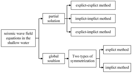
Figure 1.
Schematic diagram of solving the shallow water seismic wavefield equation.
The stability, computational accuracy and computational efficiency of the above methods are analyzed through case studies.
3. Calculation Simulation and Analysis
The calculation model of shallow water seismic wave field is shown in Figure 2. The horizontal distance of the fluid region is 200 m, the depth is 60 m, the density of the medium is 1000 kg/, and the speed of sound in the fluid is 1500 m/s; the horizontal distance of the elastic region is the same as that of the fluid region, the depth is 100 m, the density of the medium is 2300 m/s, the longitudinal wave speed is 3500 m/s, and the transverse wave speed is 1800 m/s. The sound source is located in the center of the fluid area (see solid dot in Figure 2), and a sine wave signal with a frequency of 25 Hz is used. The discretization is performed using a regular quadrilateral grid with a size of 10 m. The upper boundary of the fluid is a free surface boundary, and the rest of the boundary of the fluid–elastomer area is set as an Infinite Element Boundary (IEB) (see Figure 2). Given the simulation time and time step, the COMSOL 6.0 simulation results under the same simulation conditions are used as the “comparison solution”, and the five solution methods described in this paper are compared to compare with them to analyze the performance of this paper’s method.
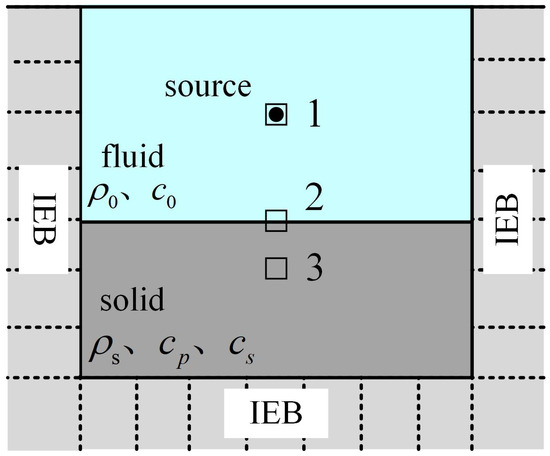
Figure 2.
Schematic diagram of the shallow water seismic wave field calculation model.
The three receiving points are shown as □ in Figure 2, where receiving point 1 is located at the sound source position. The field variables are expressed in terms of acoustic pressure, receiving point 2 is located directly below receiving point 1 at the fluid–elastomer coupling interface. The field variables are expressed in terms of acoustic pressure and displacement, respectively, and receiving point 3 is located at a depth of 40 m of the elastomer directly below receiving point 2, and the field variables are expressed in terms of displacement. The field variables are expressed in terms of displacements. In the following, the global explicit method is abbreviated as GEM, and the global implicit method is abbreviated as GIM for ease of description.
3.1. Performance Analysis
3.1.1. Stability
The method above mainly consists of the explicit center difference method and the implicit Newmark method, and the stability of these two methods is analyzed below. The explicit center difference method is a conditionally stable algorithm, and its stability conditions are [17]
where is the spectral radius, i.e., the maximum eigenvalue of the matrix, is the maximum intrinsic vibration frequency of the system, and can be obtained using the eigenvalues of the coefficient matrix.
According to the simulation conditions, the stability conditions of Equation (1), Equations (20) and (21) are calculated as , and , respectively. It can be seen that the stability of the equations in the two symmetrized forms is the same, which also reflects that symmetrizing the coefficient matrices of Equation (1) does not change the stability of the original equations from the side.
For the implicit Newmark method, when , , this method is unconditionally stable. Therefore, the unconditionally stable Newmark method is used in implicit numerical simulations.
In summary, the stability requirement of the explicit center difference method under the given conditions is about , while the implicit Newmark method is unconditionally stable, and the time step depends on the accuracy requirement.
3.1.2. Computational Efficiency
Among the partial solution methods, for the explicit–explicit method, such as Equation (10), since and are diagonal matrices, solving the inverse matrices and only needs to take the inverse of the original matrix elements, which makes the iterative solution of the field variables of linear complexity, and thus this method is the fastest; for the implicit–implicit method, such as Equation (15), it is necessary to solve and , which are non-diagonal matrices. Thus, solving the inverse matrix takes more time, plus the two equations of fluid and elastomer are solved separately and iteratively, so this method takes the longest time. For the explicit–implicit method, such as Equation (19), the iterative solution of the fluid acoustic pressure variable is of linear complexity, and the solution of the elastomer displacement field variable is of nonlinear complexity, so the solution speed of this method is located in the middle of the first two methods.
In the global solution method, from Equation (21), it can be seen that the coefficient matrices of the field variables are all non-diagonal arrays, and the solution is of non-linear complexity either by explicit or implicit methods; then, from Equations (23) and (24), it can be seen that the two solution methods need to carry out the multiplication of large matrices once, and ignoring the computation of the matrix summation, the solution time of both of them is comparable, and the later case also proves this conclusion.
3.1.3. Calculation Accuracy Expression
The computational accuracy can be given by the root mean square error (RMSE), whose expression is [18]
where N is the total number of iterations, is the simulation data of COMSOL version 6.0, s is the field variables obtained by simulation using the method in this paper, and i is the numerical index.
3.2. Performance Comparison of Different Methods
When the time is taken as 1 s and the time step is taken as 0.0001 s, the symmetrization equations expressed in Equation (20) do not converge, and the results of Equation (20) for the first 100 time steps are given in Figure 3 and Figure 4, which shows that both the sound pressure and displacement do not converge with time. This is due to the fact that when the matrix is symmetrized, since there are more degrees of freedom in the elastomer than in the fluid, the term in Equation (20) involves the operation of multiple degrees of freedom, which leads to an incomplete symmetry with the term, while the term in Equation (21) has a better symmetry with the term. Therefore, the GEM and GIM in the later study are both calculated using Equation (21).
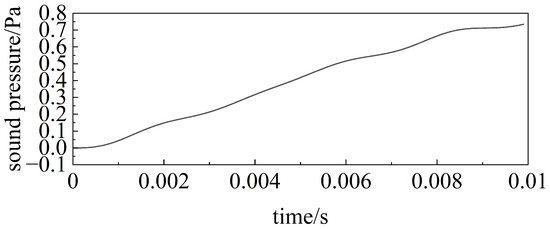
Figure 3.
Calculated results for the first 100 time steps of Equation (20) (sound pressure at reception point 1).
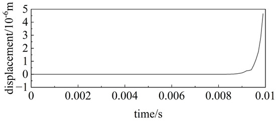
Figure 4.
Calculated results for the first 100 time steps of Equation (20) (displacement at reception point 3).
In order to facilitate the comparative analysis, the same calculation platform is used, the results are normalized, and the root mean square errors of the five methods are shown in Table 1, where represents the sound pressure at the reception point 1 in Figure 2, represents the sound pressure at the reception point 2, represents the displacement at the reception point 2, and represents the displacement at the reception point 4.

Table 1.
Root mean square error at a step size of 0.0001 s.
As can be seen from Table 1, in terms of stability, all five methods are stable because the selected step sizes satisfy the stability conditions of the explicit methods plus the unconditional stability of the implicit methods. In terms of computational accuracy, IIM and GIM have comparable accuracy because both are based on the implicit method of solving; GEM has a higher accuracy than EEM, which indicates that for the explicit method, the global solution accuracy is better than the partial solution because each iteration introduces numerical errors, and the EEM needs to be iterated in two steps (see Equation (10)), whereas the GEM can be iterated in only one step (see Equation (23)), and therefore the cumulative error of GEM is smaller than that of EEM. The accuracy of EEM is basically the same as that of EIM, which indicates that compared with the explicit–explicit method, the explicit–implicit hybrid method does not significantly improve the computational accuracy, which is due to the fact that in each iteration of EIM, the results computed by the explicit method (the first equation of Equation (19)) will be introduced to the implicit method (the second equation of Equation (19)), and the iteration of the two is nested within each other, which makes the advantage of implicit method not obvious. The advantage of the implicit method is not apparent. In terms of computational efficiency, EEM is the fastest. GEM is also an explicit method, but it involves more matrix degrees of freedom than the partial solution and takes nearly twice as long as EEM. The IIM method takes the longest time, which is about twice as long as EEM; this is because according to Equation (19), the implicit solution requires six equations to be iterated at the same time, whereas according to Equation (10), the explicit solution requires only three equations to be iterated at the same time. The time consumed by GEM and GIM is comparable, which indicates that for the global solution, the explicit method has no apparent advantage in terms of computational efficiency, because according to Equations (23) and (24), ignoring the computation of matrix summation, both GEM and GIM need to multiply large matrices once.
In order to more conveniently and intuitively show the results of the wavefield calculations, Figure 5, Figure 6, Figure 7 and Figure 8 give the results of the comparison between the GIM and COMSOL simulations at a time step of 0.0001 s. It can be seen that the field variables at each receiving point calculated by the GIM method are in very good agreement with the “comparison solution”.
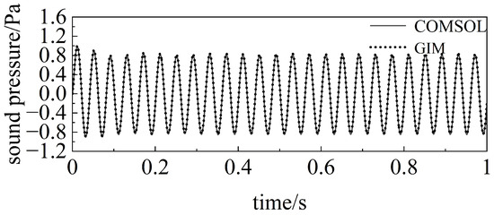
Figure 5.
GIM calculation results for a step size of 0.0001 s (sound pressure at reception point 1).
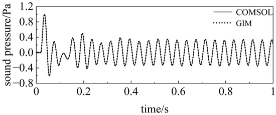
Figure 6.
GIM calculation results for a step size of 0.0001 s (sound pressure at reception point 2).
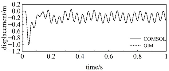
Figure 7.
GIM calculation results for a step size of 0.0001 s (displacement at reception point 2).
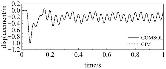
Figure 8.
GIM calculation results for a step size of 0.0001 s (displacement at reception point 3).
The root mean square error of the five methods when the time step is taken as 0.0003 s is shown in Table 2.
Table 2.
Root mean square error at a step size of 0.0003 s.
As can be seen from Table 2, since the step size is chosen close to the stability condition of the explicit method, the errors of EEM, EIM, and GEM with the explicit method increase, while the errors of the unconditional implicit methods IIM and GIM are still close to the “comparative solution”.
When the time step is 0.0004 s, the explicit method is unstable, the EEM and GEM do not satisfy the stability condition of Equation (25), and the results do not converge. Due to the mixing of implicit algorithms in EIM, the results still converge, and their root mean square errors with IIM and GIM are shown in Table 3.
Table 3.
Root mean square error at a step size of 0.0004 s.
As can be seen from Table 3, the computational errors of all three methods increase, but a comparison with the EEM in Table 1 shows that the computational accuracy of GIM at a time step of 0.0004 s is better than that of the EEM at 0.0001 s, and the time consumed is about half of that of the EEM, which at this time can reflect the advantage of the global implicit solving method at larger step sizes. When the time step is taken as 0.001 s, only IIM and GIM converge, and their root mean square errors are shown in Table 4.
Table 4.
Root mean square error at a step size of 0.001 s.
As can be seen from Table 4, the field variable errors at the coupling boundary are significantly larger for GIM compared to GIM with a step size of 0.0001 s. The acoustic pressure error in the fluid increases by 0.02, and the displacement error in the elastomer increases by about orders of magnitude. The increase in the field variable errors in the fluid and the elastomer for GIM compared to EEM with a step size of 0.0001 s is within 0.01, while the elapsed time is reduced by one-fifth.
In summary, for the time-domain solution of the shallow water seismic wave field equations, the implicit method is superior to the explicit method in terms of stability because the stability of the explicit method is limited by the time-step requirement in Equation (25), while the implicit method is unconditionally stable; the explicit method is superior to the implicit method in terms of computational efficiency because the explicit method requires only one equation to iterate for each of the field variables to be solved, e.g., the iteration of the acoustic pressure and displacement is only one equation. In terms of computational efficiency, the explicit method is superior to the implicit method because the explicit method requires only one equation for each field variable to be solved, such as Equation (10). The iteration of acoustic pressure and displacement can be realized with only one equation, whereas the implicit method requires multiple iterations, such as Equation (17). The iteration of each step includes the velocity and acceleration in addition to the field variables to be solved.
4. Conclusions
Based on the classical explicit central difference method and implicit Newmark method, this paper derives the iterative expressions of the field variables of different methods in the form of local and global solutions of the shallow water seismic wavefield equation. The numerical simulation results are verified by comparing them with the COMSOL data, and the conclusions are as follows.
- Stability: The explicit method is conditionally stable, which is more limited by the time step, and the implicit Newmark method is unconditionally stable. Under the guarantee of accuracy, the implicit method of the global solution is the optimal choice both in terms of accuracy and efficiency.
- Computational efficiency: In the global solving method, the explicit and implicit methods are comparable in terms of time consumption. In the local solving method, the explicit–explicit method and the explicit–implicit hybrid method are comparable in terms of time consumption, and the implicit–implicit method consumes three times as much time as the former two. Under the same time step, the local solving implicit–implicit method takes the most time, and the global solving method takes more time than the other local solving methods.
- Computational accuracy: For the same time step, the accuracy of the implicit method is better than the explicit method in both local and global solving methods. The accuracy of the explicit method in global solving is better than that of the explicit method in local solving, and the accuracy of the implicit method in global solving with a large step size is comparable to that of the explicit–explicit method in local solving with a small step size for different time steps.
In this paper, the optimal solution of the shallow water seismic wavefield equation is given based on the classical explicit center difference and implicit Newmark methods, which also apply to solving similar problems with fluid–elastomer coupling. The next step will be to investigate the solution method with higher accuracy and efficiency in the case of unconditional stability.
Author Contributions
Conceptualization, W.C.; methodology, W.C.; writing—original draft preparation, W.C.; writing—review and editing, G.C. and Y.C.; funding acquisition, B.L. All authors have read and agreed to the published version of the manuscript.
Funding
This research was funded by the National Natural Science Foundation of China: 12104510; General Program of China Postdoctoral Science Foundation: 2022M723882.
Institutional Review Board Statement
Not applicable.
Informed Consent Statement
Not applicable.
Data Availability Statement
Dataset available on request from the authors.
Conflicts of Interest
The authors declare no conflicts of interest.
References
- Si, J.G.; Feng, H.X.; Su, J.; Tang, S.B.; Zhange, J.X.; Li, Z.C. Research on shallow sea detection technology based on seismic wave. Prog. Geophys. 2022, 36, 2596–2603. [Google Scholar]
- Sun, Q.P.; Zhou, H. Real-time Detection Algorithm for Ship Seismic Wave Signal Based on HHT. Digit. Ocean. Underw. Warf. 2021, 4, 310–317. [Google Scholar]
- Zhang, Z.P.; Li, H.; Shao, Y.X.; Wu, Q. Study on Method of Target Recognition in Water of Seabed Seismic Wave. J. Shenyang Ligong Univ. 2017, 36, 38–43. [Google Scholar]
- Lu-Wen, M.; Guang-Li, C.; Ya-Nan, C.; Ming-Min, Z. On the Porpogation Mechanism of Ship Seismic Wave and Its Application in Mine Fuze. Acta Armamenta 2017, 38, 319–325. [Google Scholar]
- Cheng, G.L.; Tang, K.; Liu, B. On fast prediction method of seabed seismic wave induced by spherical sound source in shallow water. J. Nav. Univ. Eng. 2023, 35, 6–12. [Google Scholar]
- Ren, B.; Wu, Q.; Zhang, Z.P. Numerical simulation study of seismic waves in ships based on flow-solid coupling. Electron. World 2017, 17, 19–20. [Google Scholar]
- Wang, X.C. Finite Element Method, 1st ed.; Tsinghua University Press: Beijing, China, 2003; pp. 476–482. [Google Scholar]
- Zhu, C.Y.; Qin, G.L.; Xu, Z. Comparison of Explicit Central Difference Method and Implicit Newmark Method Using Chebyshev Spectral Element Method for Wave Equations. J. Xi’an Jiaotong Univ. 2008, 9, 1142–1145. [Google Scholar]
- Elena, Z.; Luca, F.P. Explicit second order isogeometric discretizations for acoustic wave problems. Comput. Methods Appl. Mech. Eng. 2019, 348, 776–795. [Google Scholar]
- Zhou, H. A new time-marching scheme that suppresses spurious oscillations in the dynamic rupture problem of the spectral element method: The weighted velocity Newmark scheme. Geophys. J. Int. 2015, 203, 927–942. [Google Scholar] [CrossRef]
- Ji, Y.; Xing, Y.F. A Two-Sub-Step Generalized Central Difference Method for General Dynamics. Int. J. Struct. Stab. Dyn. 2020, 20, 2050071. [Google Scholar] [CrossRef]
- Huang, Z.L.; Chen, S.L.; Shen, J.R.; Zhang, L.F. Three-dimensional Large-scale Marine Seismic Response Analysis Based on the Unified Computational Framework of Fluid-solid Interaction—A Case Study of Tokyo Bay. Technol. Earthq. Disaster Prev. 2022, 17, 420–430. [Google Scholar]
- Yang, Y.Q.; Zhu, L.S.; Tang, S.R. Study on Fluid-Structure Interaction for Submerged Flexible Short Plate Based on Numerical Wave Tank. Shipbuild. China 2022, 63, 41–51. [Google Scholar]
- Liu, C.; Guo, L.F.; Yuan, Y.; Zhou, A.H.; Liu, X.D. Calculation Model of Vertical Deformation of Ground Fracture Caused by Pumping Based on Fluid-Solid Coupling. J. Hebei Univ. Geol. 2022, 45, 50–55. [Google Scholar]
- Chen, S.L.; Cheng, S.L.; Ke, X.F. A unified computational framework for fluid-solid coupling in marine earthquake engineering: Irregular interface case. Chin. J. Theor. Appl. Mech. 2019, 51, 1517–1529. [Google Scholar]
- Komatitsch, D.; Barnes, C.; Tromp, J. Wave propagation near a fluid-solid interface: A spectral element approach. Geophysics 2000, 65, 623–631. [Google Scholar] [CrossRef]
- He, Q.; Gan, H.; Jiao, D. Explicit Time-Domain Finite-Element Method Stabilized for an Arbitrarily Large Time Step. IEEE Trans. Antennas Propag. 2012, 60, 5240–5250. [Google Scholar] [CrossRef]
- Wang, J.J.; Li, J.H.; Yan, S.F.; Shi, W.; Yang, X.; Guo, Y.; Gulliver, T.A. A Novel Underwater Acoustic Signal Denoising Algorithm for Gaussian/Non-Gaussian Impulsive Noise. IEEE Trans. Veh. Technol. 2021, 70, 429–445. [Google Scholar] [CrossRef]
Disclaimer/Publisher’s Note: The statements, opinions and data contained in all publications are solely those of the individual author(s) and contributor(s) and not of MDPI and/or the editor(s). MDPI and/or the editor(s) disclaim responsibility for any injury to people or property resulting from any ideas, methods, instructions or products referred to in the content. |
© 2024 by the authors. Licensee MDPI, Basel, Switzerland. This article is an open access article distributed under the terms and conditions of the Creative Commons Attribution (CC BY) license (https://creativecommons.org/licenses/by/4.0/).