Numerical Determination of the Load-Bearing Capacity of a Perforated Thin-Walled Beam in a Structural System with a Steel Grating

Abstract

This article presents the results of numerical simulations of a structural system consisting of steel perforated thin-walled beams and a steel grating. The simulations were conducted using the finite element method. The analysis took into account physical and geometric nonlinearity as well as the contact between the steel grating and the beams. The main goal of the research was to develop load-bearing curves for the main beam in the span range of 3–6 m and to identify destruction patterns depending on the span of the structural system. For the purpose of validating the developed numerical model, laboratory tests were conducted on two structural systems with spans of 3 m and 6 m, as well as tests on the strength parameters of the material taken from the tested beams. The laboratory tests confirmed the correctness of the proposed numerical model, which allowed for the simulation of the behavior of the structural system in the full range of spans.

1. Introduction

Since the introduction of steel as a construction material in the building industry, this material has been continuously refined to improve its properties by creating alloys with greater strength and ductility. The aim of these innovations was to achieve the appropriate strength necessary for structural elements used in construction. Structural steel elements, which can be shaped in the process of hot rolling or cold forming from thin sheets, have also evolved through the development of various cross-sectional forms. Cold-formed steel shapes are produced from thin steel sheets using an edge press or a roll forming process, by passing the sheet through several dies. A distinguishing feature of thin-walled shapes from hot-rolled steel shapes is that the load is carried by the shape of the section, not the thickness of the section [1].

The first use of thin-walled profiles dates back to 1850, but their use in construction gained acceptance only after 1925. Design standards for hot-rolled steel began to appear after 1930, but they were not adapted for the design of thin-walled elements. In the USA, the first guidelines for designing lightweight structures with thin-walled profiles were developed based on research conducted at Cornell University, which was published in 1946 [2]. Many countries adopt American standards, while European Union countries use Eurocode 3 [3,4,5,6]. In the last twenty years, structures using cold-rolled thin-walled profiles have become increasingly popular. Their numerous advantages compared with other building materials, combined with advances in their production technologies, have contributed to the popularity of these solutions in industrial construction, including in areas prone to seismic activity. Steel thin-walled profiles are increasingly used for constructing high storage racks as well as mezzanines and platforms. These structures are used in the development of internal spaces of warehouse and production halls.

Cold-rolled steel products are manufactured at ambient temperature, and the technological process of producing such profiles contributes to their high strength and low weight. This, in turn, increases the ease of assembly and facilitates the logistics associated with transporting components to the construction site. However, their specific thin-walled construction means that their strength properties may be susceptible to changes in geometry [7]. Even though tolerances in the production process are strictly controlled, factors such as transportation and storage can contribute to the introduction of additional imperfections in the geometry of thin-walled elements [8,9]. This makes predicting the behavior of structures more complicated due to random geometric changes that may occur during numerical simulations. Standard computer simulations usually assume initial imperfections in thin-walled models, based on the first buckling modes [10]. Their magnitude is set as L/960 both in Chinese regulations [11] and North American standards [10]. Accurate simulations predicting strength must take into account the real working conditions of thin-walled elements and, above all, their original geometry.

There are several computational methods that can be applied in the analysis of structures made of thin-walled profiles: The Generalized Beam Theory (GBT), specifically designed for the analysis of thin-walled rod structures. The GBT effectively deals with complex deformations and buckling in such elements [12,13,14,15]. The SAFSM (semi-analytical finite strip method) [16] is a semi-analytical structural analysis method for thin-walled elements. This method involves dividing the element into many strips, in which it is assumed that displacements are linear functions. This allows for an analytical solution in the direction perpendicular to the axis of the element and numerical along it. The constrained finite strip method (cFSM) [17] is an extension of the semi-analytical finite strip method (SAFSM) for structural analysis of thin-walled elements. It allows for the creation of constraint matrices by considering displacement fields and various mechanical criteria. Applying these constraint matrices to the eigenvalue problem of linear buckling in the SAFSM leads to strain fields that meet the considered criteria and isolate specific modes. By carefully selecting mechanical criteria, the resulting strain fields can be limited to specific buckling modes. This is known as modal decomposition.

Structural elements made of thin-walled profiles often also feature perforation. This perforation is not used to reduce the weight of the element as is often the case with hot-rolled profiles, but is necessary for technological reasons, such as accommodating essential installations. The presence of perforations is another factor that complicates the accurate estimation of the load-bearing capacity of such elements. The use of computational methods like the GBT, SAFSM, or cFSM in the case of perforated elements can be challenging or may come with certain limitations. Although there are studies showing that such limitations can be overcome [18], in the case of perforated thin-walled elements, it is particularly important to accurately consider local weaknesses and stress concentrations around the holes. Methods like the finite element method (FEM) are often more suitable for such analyses, as they allow for more detailed modeling of local effects and are undoubtedly more popular and widespread in the engineering community.

It is also important to take into account in the calculations the fact of the cooperation of the analyzed element with neighboring elements, the susceptibility of bridges connecting cooperating elements, and the influence of the strength of connectors (connecting elements) on the behavior of the entire structural system, and consequently the influence of all these factors on the load capacity of a single structural element. Including all these effects is possible thanks to the use of a model based on the finite element method. Such a model, to be credible, must be validated by laboratory tests. This approach was used in this work to estimate the load capacity of a thin-walled perforated beam working in a structural system with a steel grating.

2. Materials and Methods

The primary goal of the research was to estimate the load-bearing capacity of the central beam working in the analyzed structural system with a linear load transferred by steel gratings placed over the entire span of the beams. Due to the costs of laboratory tests and the difficulty in obtaining a linear load over the entire length of the tested beam during the test, the following research program was adopted:

Laboratory tests necessary for the validation of the numerical model:

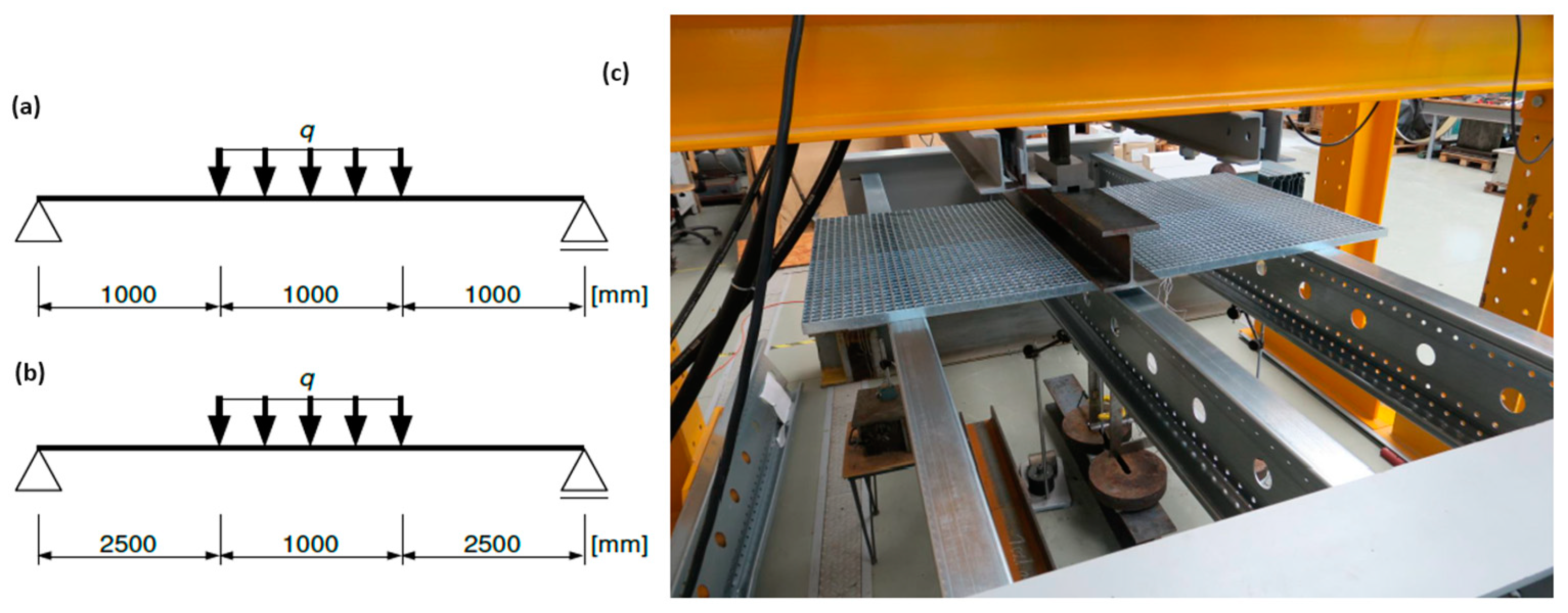
• Laboratory tests of a 3 m-span structural system with a load transferred to the system through a single steel grating.
• Laboratory tests of a 6 m-span structural system with a load transferred to the system through a single steel grating.
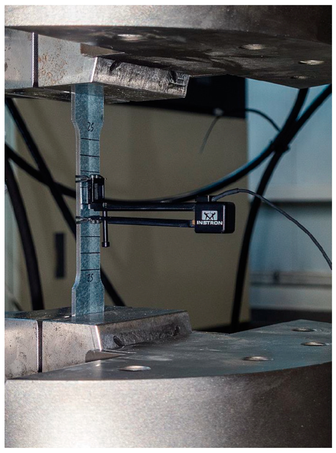
• Laboratory tests of the strength properties of the steel from which the beams and connectors were made.

Numerical simulations:

• Development and validation of a 3 m-span structural system model.
• Development and validation of a 6 m-span structural system model.
• Development of structural system models for spans of 3.0 m, 3.5 m, 4.0 m, 4.5 m, 5.0 m, 5.5 m, and 6.0 m with a load transferred by steel gratings placed over the entire span.
• Conducting simulations to determine load-bearing curves.

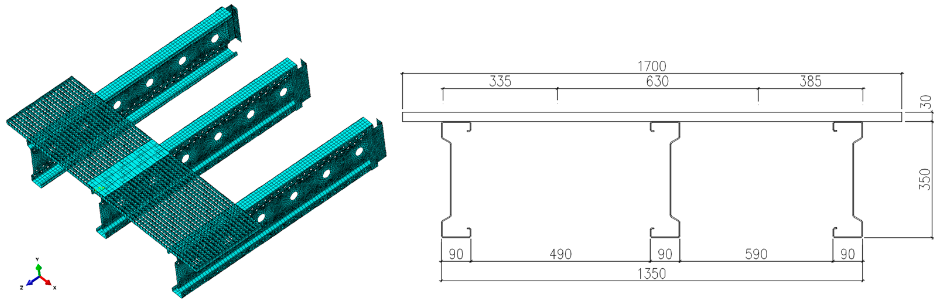
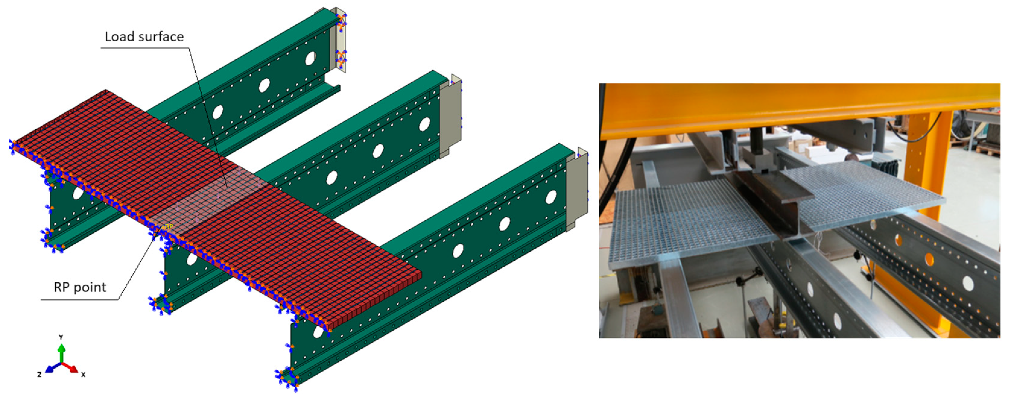
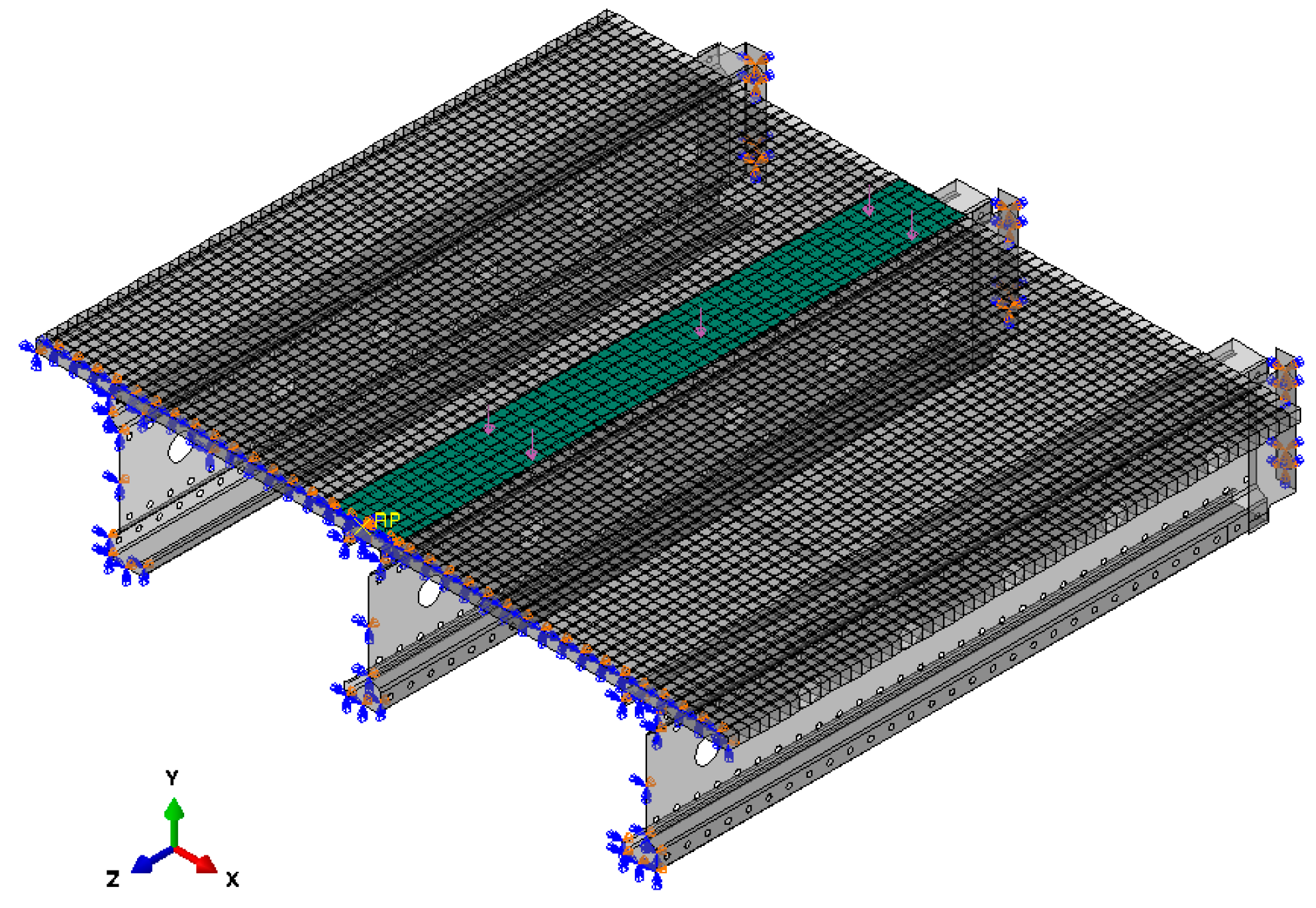
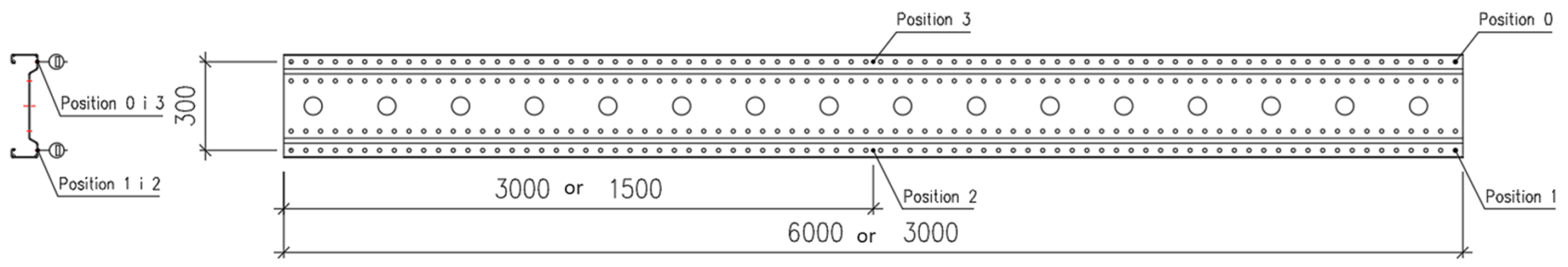
2.1. Numerical Model

The numerical model was created using the Abaqus Simulia 2022 software [19], which employs the finite element method for calculations. The entire geometry of the system was modeled using shell-type surface elements [19], with an effort to replicate the real conditions of laboratory tests as closely as possible. The dimensions and mutual positioning of the model elements were identical to the real-life conditions. The model utilized the symmetry of the system to reduce the size of the task and the time consumption of calculations. The mutual positioning of the model elements is shown in Figure 1, which represents half of the analyzed system (utilizing task symmetry). The variable parameter of the model’s geometry was the length of the beams.

For modeling the geometry of the system, finite elements S4R (a 4-node doubly curved thin or thick shell, reduced integration, hourglass control, finite membrane strains) from the Abaqus 2022 software library [19] were used. Figure 1 shows the discretization of the system with a 3 m-long beam. An automatic meshing technique using a progressive front algorithm was applied to generate the finite element mesh throughout the model. This technique generated the mesh from the boundaries of the geometry and extended it deep into the model area. This allowed control of the mesh density and ensured good-quality elements with complex shapes. The generated mesh consisted of quadrilateral elements. The number of elements depended on the span; for a system with a span of 3 m there were 36,815 elements, and for a span of 6 m there were 65,171 finite elements. The following boundary conditions were applied in the model:

• Connectors were fixed at the location of mounting holes on a surface with a diameter of 40 mm.
• Connectors were connected to the beams using a “Tie”-type contact [19], which corresponds to a rigid connection of the connector to the beam.
• Symmetric boundary conditions were applied to the axis of symmetry of the system on the steel grating and beams.

In the model, a “General contact” type [19] was used between the bridge deck and the beams. The following contact parameters were adopted:

• Normal Behavior—“Hard” Contact.
• Tangential Behavior—Penalty, Friction coefficient = 0.3.

The steel grating was modeled with real dimensions. The only simplification applied was the substitution of the round cross-section transverse rods with square cross-sections with the same surface area.

The load in the form of a concentrated force applied at the RP point, generated by the strength testing machine, was modeled as a Pressure load, evenly distributed over a surface 160 mm wide, which corresponded to the real conditions during the test. The method of loading the system is shown in Figure 2. During the validation of the model, an ideally elastic–plastic material was assumed with the following parameters.

For the beams:

• Young’s modulus E = 205.5 GPa, determined based on laboratory tests.
• Poisson’s ratio ν = 0.3.
• Yield strength R_H = 490 MPa, determined based on laboratory tests.

For the connectors and the steel grating:

• Young’s modulus E = 200 GPa, determined based on laboratory tests.
• Poisson’s ratio ν = 0.3.
• Yield strength R_H = 362 MPa, determined based on laboratory tests.

In real structural conditions, thin-walled beams often exhibit imperfections resulting from manufacturing processes, assembly, and natural characteristics of the material. Such imperfections significantly influence the behavior of the structure, especially in terms of sensitivity to buckling and other nonlinear effects. Incorporating these imperfections into the analysis allows for a more realistic and reliable simulation, which is crucial for the safety and durability of the structure. Additionally, this is in line with the recommendations of engineering standards and allows for a more accurate prediction and understanding of the critical operating conditions of the beams. In the presented approach, imperfections were introduced into the model based on the first mode of buckling. In Abaqus 2022 software, the introduction of geometric imperfections based on the first buckling mode begins by performing a linear buckling analysis on the ideal model to identify the shapes and values of critical buckling forces. The selected first buckling mode is then scaled to a specific value representing the allowable imperfections for the structure. In the presented model, a factor equal to 1/300 of the beam length was assumed. This scaled buckling form was then used as a geometric modification of the model. Finally, a nonlinear analysis was carried out, taking into account the introduced imperfections, to evaluate the impact of these changes on the behavior of the structure under load.

2.2. Numerical Model Used to Develop Load-Bearing Curves for the Central Beam

To estimate the load-bearing capacity of a thin-walled perforated beam with a length ranging from 3 m to 6 m, continuously loaded in the validated model, one change was made to more accurately simulate the real working conditions of such an element. Namely, the steel grating was extended according to Figure 3. The steel grating ends 100 mm before the end of the beams. However, the load is still applied over a 160 mm wide band. This band is deformable with a thickness of 1 mm and material parameters like the steel grating. Such a distribution of the load negates the stress concentration that would occur with the use of linear loading [N/mm]. This type of load can be obtained from a simple calculation: $q=p·160·x$, where q is the continuous load acting on the beam [N/mm], p is the surface load [N/mm²] acting on a band 160 mm wide, and x is a scaling factor for the load q in relation to the actual percentage value of the load taken over by the central beam, e.g., x = 0.6 for 60% according to

Table 1. Percentage amount of load taken over by individual beams calculated based on the comparison of deflections.

Load Taken over by the Right Beam [%]	Load Taken over by the Central Beam [%]	Load Taken over by the Left Beam [%]	Length of the Beam [m]
1.284	89.514	9.203	3.0
1.903	89.582	8.515	3.5
3.481	86.969	9.55	4.0
4.368	85.925	9.706	4.5
3.682	87.064	9.254	5.0
3.593	87.799	8.608	5.5
3.501	87.825	8.674	6.0

. The percentage value of the load borne by the central beam was determined based on a comparison of deflections. This was achieved when LE Max. Principal (Abs) = 5% [19] was reached in the model, where LE Max. Principal (Abs) is the logarithmic measure of strain. The use of logarithmic strains is particularly useful in analyses where traditional, small linear strains are not accurate enough.

2.3. Laboratory Tests

Laboratory tests of the structural system and determination of the real modulus of elasticity of the material and yield strength were performed using the INSTRON 8804 strength testing machine. In the case of testing the structural system, a static bending scheme was adopted with a load distributed over part of the beam length (1.0 m) according to Figure 4. In the middle of the beam span and at the connector, displacement measurement systems were prepared as shown in Figure 5. The displacements were measured with SYLVIAC sensors placed on the side of the beam.

The loading scheme was as follows:

• Loading to achieve a displacement value of the actuator of the strength testing machine equal to 7.0 mm over 70.0 s for the 3 m beam and 15.0 mm over 150.0 s for the 6 m beams (speed: 0.1 mm/s);
• Unloading to a displacement value of the actuator of the machine equal to 0.0 mm over 70.0 s for the 3 m beam and 150.0 s for the 6 m beams (speed: 0.1 mm/s);
• Elastic phase, in which the displacement value of the actuator was increased from 0.0 mm to 7.0 mm over 70.0 s for the 3 m beam and 15.0 mm over 150.0 s for the 6 m beams (speed: 0.1 mm/s); during this phase, measurements of beam and connector displacements and force were made, and a deflection–force diagram was plotted;
• Destruction phase; after conducting the test of beam operation in the elastic range, the sample was unloaded to a displacement value of the actuator of the strength testing machine equal to 0.0 mm and then loaded until destruction at a speed of 0.1 mm/s. During the test, a deflection–force diagram was plotted.

While determining the strength parameters of the materials, a static scheme of a stretched rod was adopted. An extensometer with a measurement base of 24.1 mm was placed inside the pure tension zone, as shown in Figure 6. The samples were loaded according to the following scheme:

• Loading to achieve a displacement value of the actuator of the strength testing machine equal to 0.3 mm over 60.0 s (speed: 0.3 mm/min);
• Unloading to a displacement value of the actuator of the machine equal to 0.0 mm over 60.0 s (speed: 0.3 mm/min);
• Main phase, in which the displacement value of the actuator was increased from 0.0 mm to 0.3 mm over 60.0 s (speed: 0.3 mm/min); during this phase, measurements of the elongation of the sample and the increase in force were made, and a deflection–force diagram was plotted.

3. Results and Discussion

This section presents the results of the validation of the numerical model based on the laboratory tests carried out, as well as the results of the targeted numerical simulations.

3.1. Results of Laboratory Tests

During the laboratory tests, a total of six structural systems were tested (Figure 7, Figure 8, Figure 9, Figure 10, Figure 11, Figure 12, Figure 13, Figure 14, Figure 15 and Figure 16), three each of 3 m and 6 m lengths. The averaged deflection–force relationship in determining the load-bearing capacity from all tested structural systems is shown in Figure 17.

Material tests were conducted on a total of 18 samples, with 6 each cut from the top flange, web of the beam, and connectors. The material sample tests showed that the average longitudinal modulus of elasticity for the steel of the beams was 205.526 GPa and for the steel of the connectors 199.603 MPa, which is within the typical range of values for steel ranging from 200 to 210 GPa. The average yield strength for the steel from which the beams were made was 490.000 MPa, while for the steel of the connectors it was 362.000 MPa.

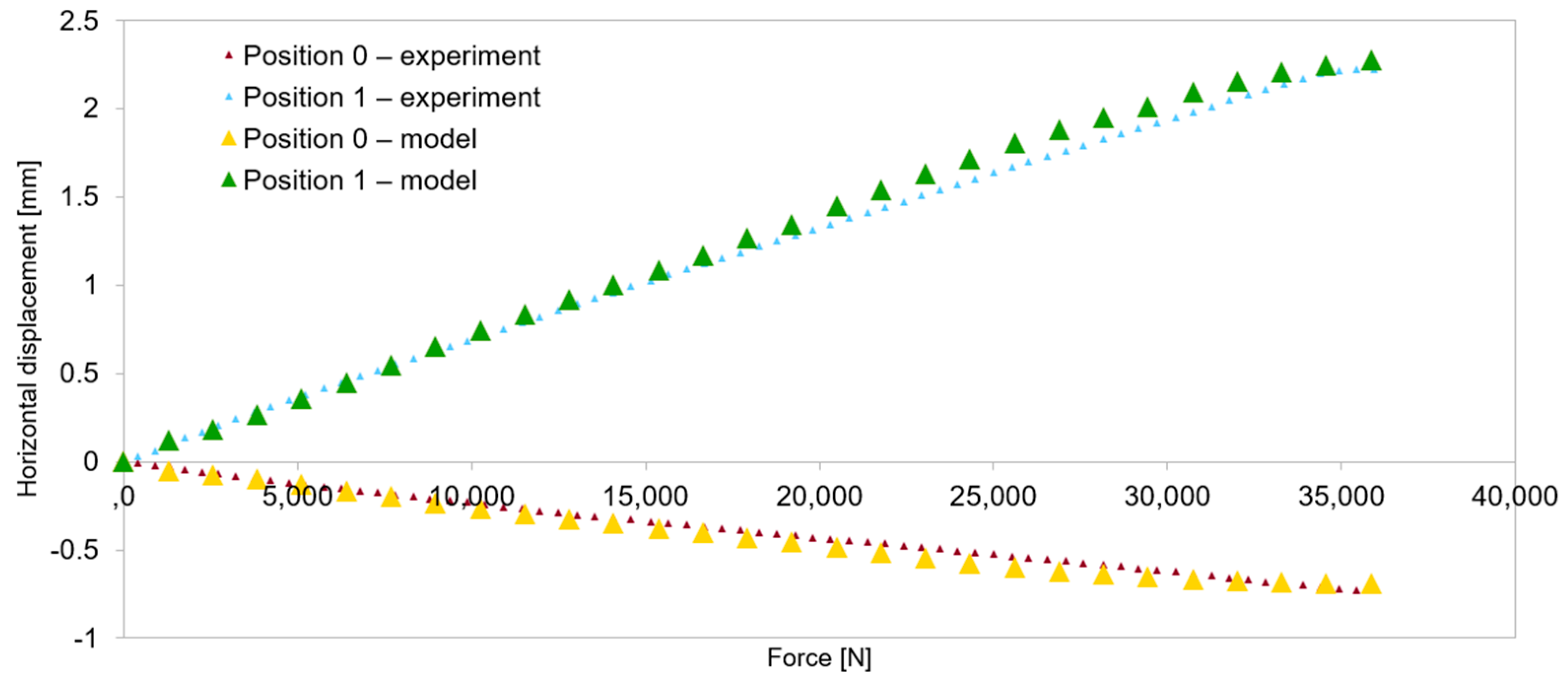
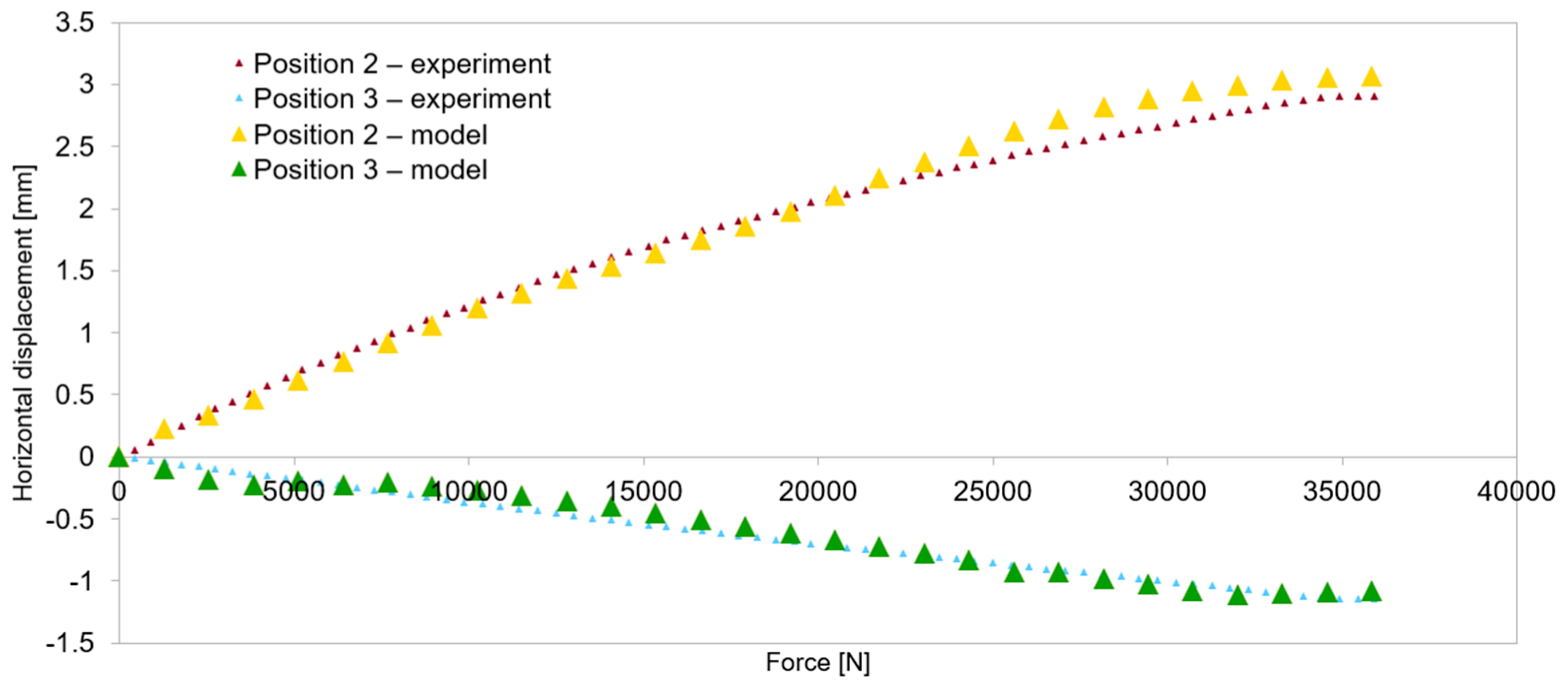
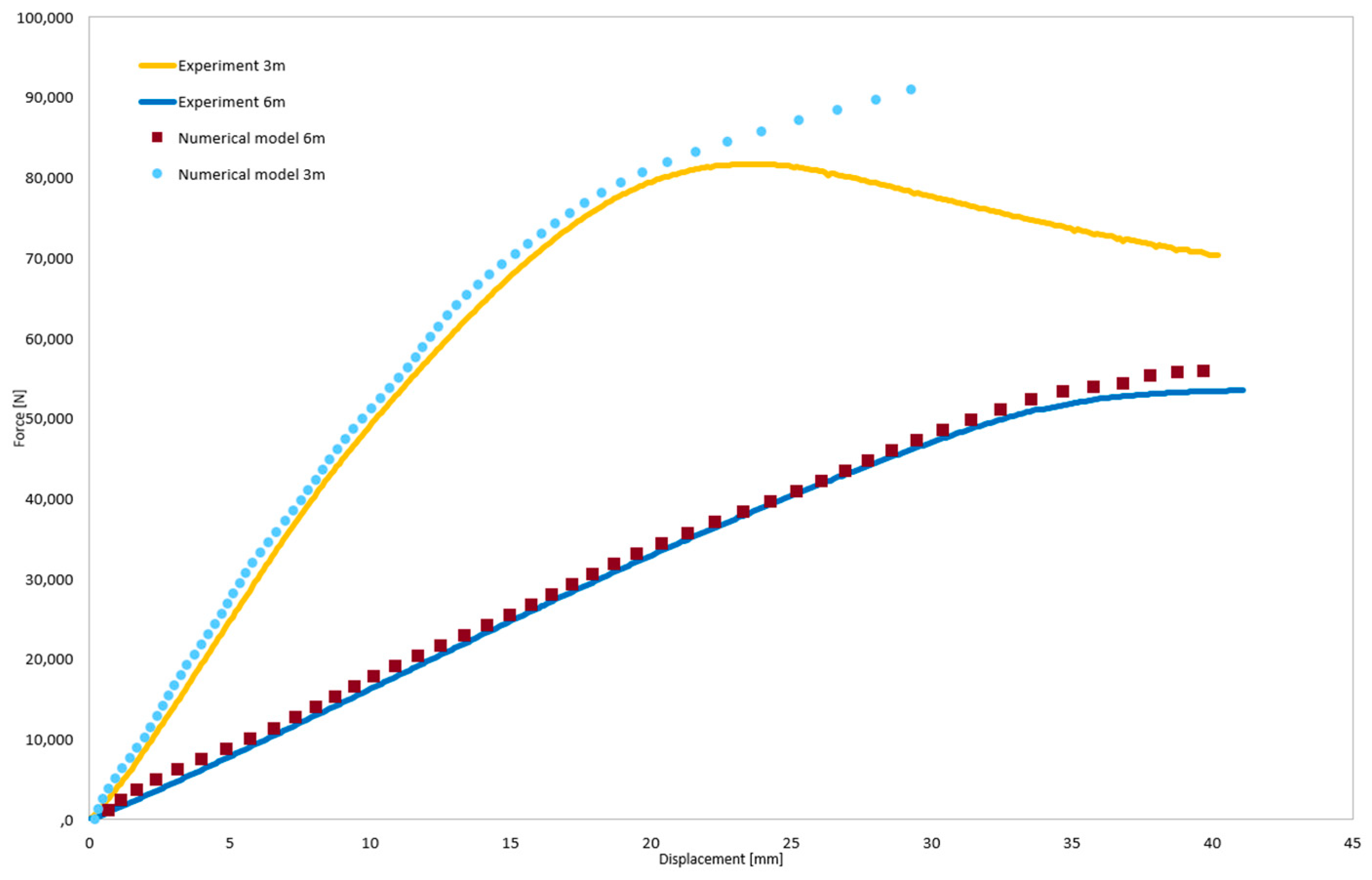
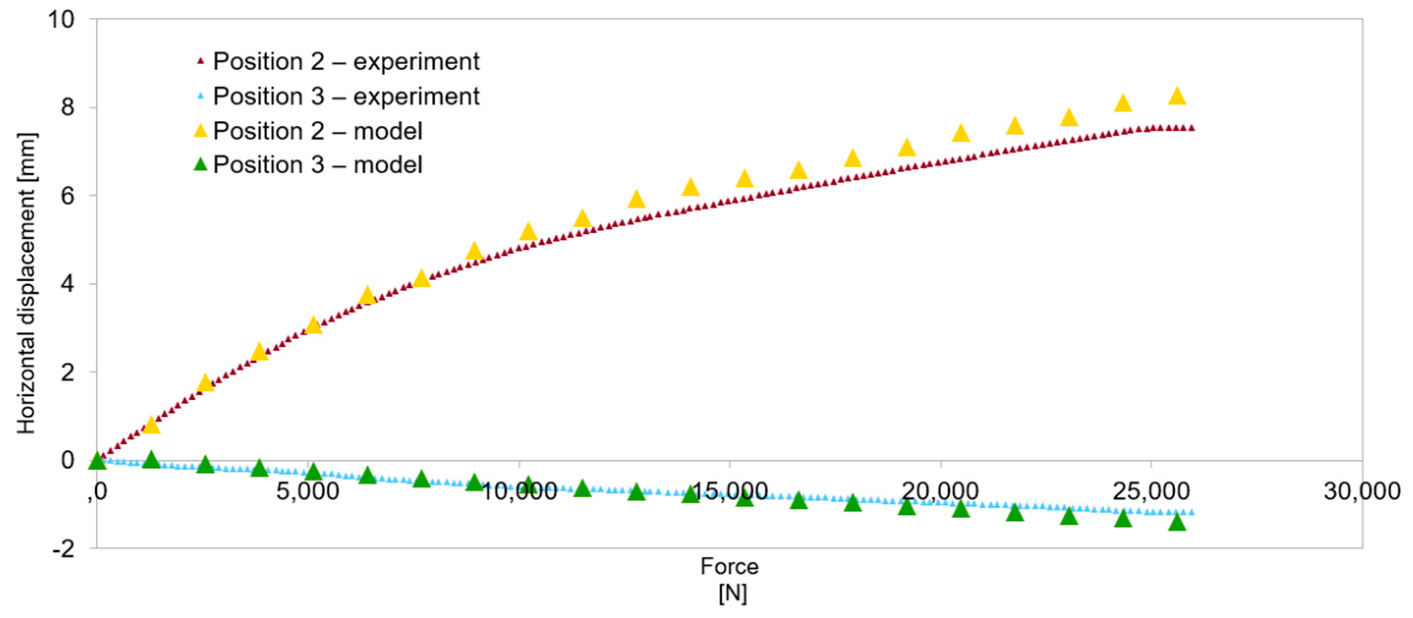
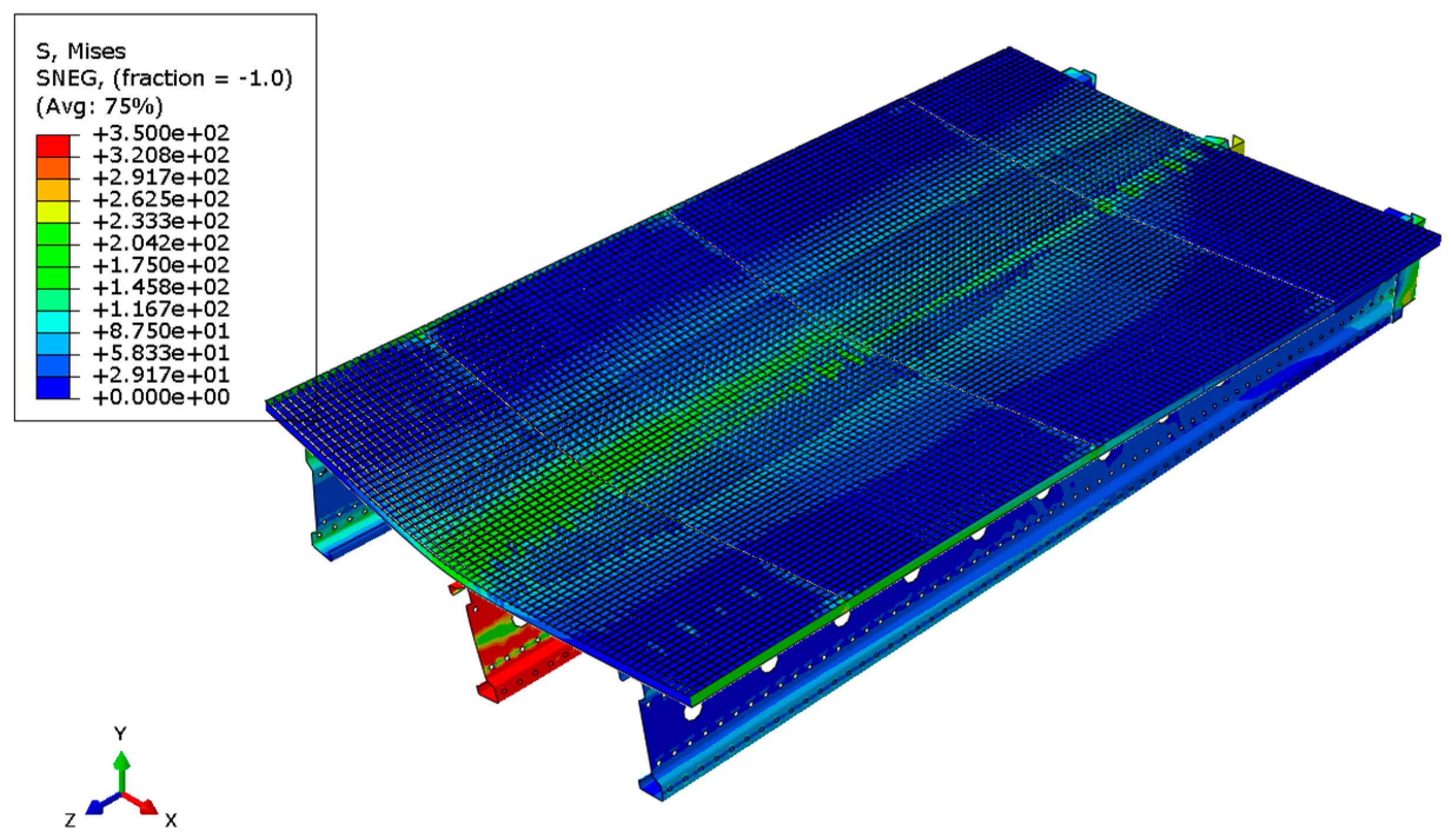
3.2. Results of Numerical Simulations and Model Validation

Analyzing the stress distributions and deformations of the systems shown in Figure 7, Figure 8, Figure 9, Figure 10, Figure 11 and Figure 12, it can be observed that in the case of the 3 m beam, the loss of load-bearing capacity is a result of the material yielding in the central zone of the beam (red color) as well as at the connector–beam junction and the connector itself. In the case of the 6 m beams, a different pattern of load-bearing capacity loss is observed. The beams do not yield in the central or support zones but undergo buckling. In the case of both the 3 m and 6 m beams, the connector yields each time. Similar effects were also observed during experimental tests as shown in Figure 10 and Figure 11.

Figure 7. Reduced Mises stress distribution for a 3 m beam.

Figure 7. Reduced Mises stress distribution for a 3 m beam.

Figure 8. Reduced Mises stress distribution for a 3 m beam—cross-section.

Figure 8. Reduced Mises stress distribution for a 3 m beam—cross-section.

Figure 9. Reduced Mises stress distribution for a 6 m beam.

Figure 9. Reduced Mises stress distribution for a 6 m beam.

Figure 10. Reduced Mises stress distribution for a 6 m beam—cross-section.

Figure 10. Reduced Mises stress distribution for a 6 m beam—cross-section.

Validation in numerical simulations is essential as it ensures the credibility of the results, helps understand the limitations of the model, and contributes to its refinement, thereby increasing the accuracy and utility of the simulations. In the present study, model validation was performed through both qualitative and quantitative comparisons. The qualitative comparison involved checking whether the same behavior of the analyzed structural system was observed in both the experiment and numerical simulations. The results of these comparisons are presented in Figure 11 and Figure 12. These clearly show different forms of destruction through buckling of the beam or material yielding.

Figure 11. Loss of stability (buckling) of the central 6 m beam.

Figure 11. Loss of stability (buckling) of the central 6 m beam.

Figure 12. Yielding in the middle of the span of the central 3 m beam.

Figure 12. Yielding in the middle of the span of the central 3 m beam.

Quantitative validation involved comparing horizontal displacements and force–displacement graphs. During the tests in the elastic range of beam operation, horizontal displacements were recorded. The distribution of the measurement points is shown in Figure 5. Figure 13, Figure 14, Figure 15 and Figure 16 present the values of horizontal displacements for each measurement point. The graphs were prepared based on the average values from all tests conducted in the elastic range of beam operation and the results obtained from the numerical model.

Figure 13. Model validation—horizontal displacements of the support cross-section for the 3 m beam.

Figure 13. Model validation—horizontal displacements of the support cross-section for the 3 m beam.

Figure 14. Model validation—horizontal displacements of the central cross-section for the 3 m beam.

Figure 14. Model validation—horizontal displacements of the central cross-section for the 3 m beam.

Figure 15. Model validation—horizontal displacements of the support cross-section for the 6 m beam.

Figure 15. Model validation—horizontal displacements of the support cross-section for the 6 m beam.

Figure 16. Model validation—horizontal displacements of the central cross-section for the 6 m beam.

Figure 16. Model validation—horizontal displacements of the central cross-section for the 6 m beam.

The final confirmation of the correctness of the numerical model was the comparison of the force–displacement relationships obtained from experimental tests and computer simulations. These are shown in Figure 17.

Figure 17. Model validation—force–displacement relationship for the RP point.

Figure 17. Model validation—force–displacement relationship for the RP point.

The discrepancy between the laboratory test results and the numerical model for the 3 m-long beams at higher displacement values is due to the material models adopted in the numerical simulations. These are linear elastic–plastic models without damage. Such models in numerical simulation do not reproduce the actual force–displacement curve at higher displacement values. However, these models are sufficient to capture the onset of material yielding.

Analyzing the presented results, it can be concluded that the adopted model simulates the real system with satisfactory accuracy, and further numerical simulations can be conducted based on it. In all cases, the discrepancies between the numerical model and experimental tests did not exceed 10%.

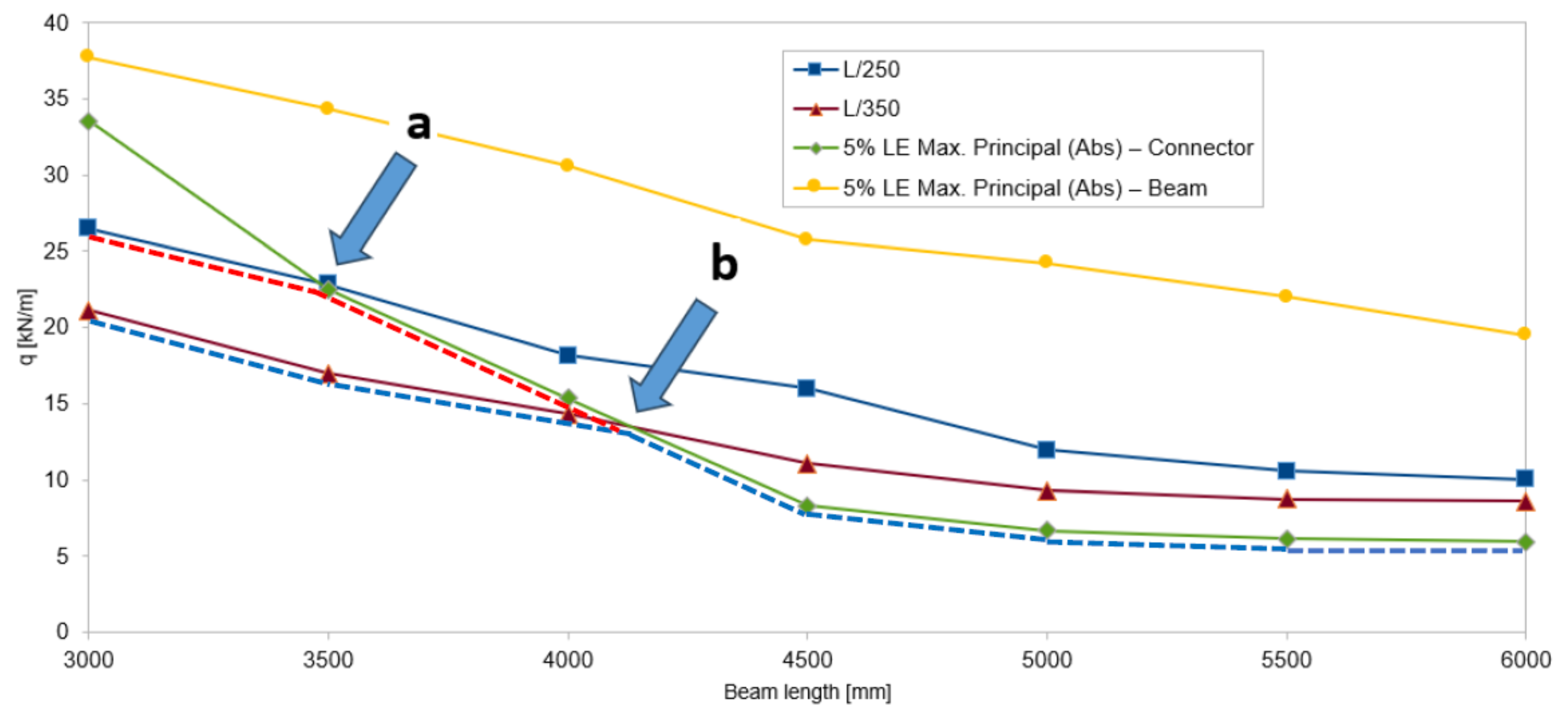
3.3. Results of Targeted Numerical Simulations

The aim of the numerical simulations was to estimate the load-bearing capacity of a thin-walled perforated central beam, with a span ranging from 3 m to 6 m, working in the analyzed structural system with a linear load transferred by steel gratings placed over the entire span of the beams. The limit values for deflection in the middle of the span of the central beam, L/250 or L/350, were adopted as the criterion for exhaustion of the load-bearing capacity. Given that the connector was identified as the weakest element of the structural system, both in the laboratory tests and numerical simulations, an additional criterion for exhaustion of the load-bearing capacity was set as reaching 5% LE Max. Principal (Abs) [19] in the connector. LE Max. Principal (Abs) is a logarithmic measure of strain. Nominal values of the material strength parameters were used for calculations at this stage.

For the beams:

• Young’s modulus E = 200 GPa.
• Poisson’s ratio ν = 0.3.
• Yield strength R_H = 350 MPa.

For the connectors and the steel grating:

• Young’s modulus E = 200 GPa.
• Poisson’s ratio ν = 0.3.
• Yield strength R_H = 235 MPa.

Figure 18, Figure 19, Figure 20, Figure 21, Figure 22 and Figure 23 show the distribution of reduced Mises stresses and the deformation of the system for the last step of the numerical analysis.

Analyzing the results of the simulations, it can be observed that in all cases the weakest element of the system is the connector, which yields first. Subsequently, the support zones of the beams yield, leading to the loss of stability of the central cross-sections. Figure 24 presents the load-bearing curves for four criteria: L/250, L/350, and 5% LE Max. Principal (Abs) achieved in the connector and the central beam.

The intersection points marked as a and b on the load-bearing curves can be termed as turning points, defining the actual progression of the load-bearing curves. For beams with lengths from 3 m to 3.5 m, we can estimate the limit load for the criteria L/250 and L/350 from Figure 24. For beams longer than 3.5 m, the L/250 criterion becomes unattainable because the 5% LE Max. Principal (Abs) in the connector will be reached before such deflection at the middle of the central beam’s span is achieved. From point a to point b, the load-bearing capacity is limited by the L/350 condition and the limit deformation value in the connector. Meanwhile, from point b, i.e., for beam spans around 4.1 m, the load-bearing capacity is determined solely by the limit deformation of the connector.

4. Conclusions

This article pertains to the numerical simulation of a thin-walled perforated beam working in a structural system with a steel grating. The main objective of the study was to develop the load-bearing curves shown in Figure 24 for the main beam within the span range of 3–6 m and to identify patterns of destruction depending on the span of the system. The validation of the developed numerical model through laboratory tests confirmed its accuracy and enabled the simulation of the behavior of the structural system covered with steel gratings over the entire span. Based on the conducted analyses, the following final conclusions can be formulated:

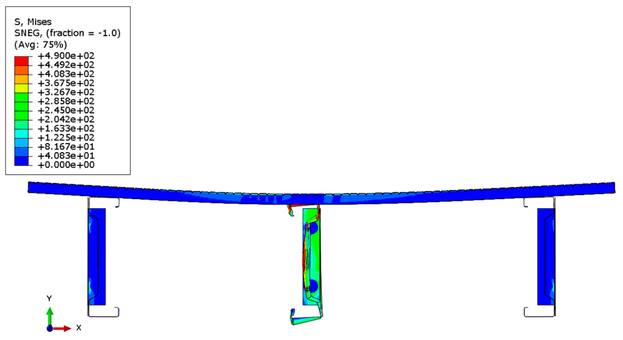
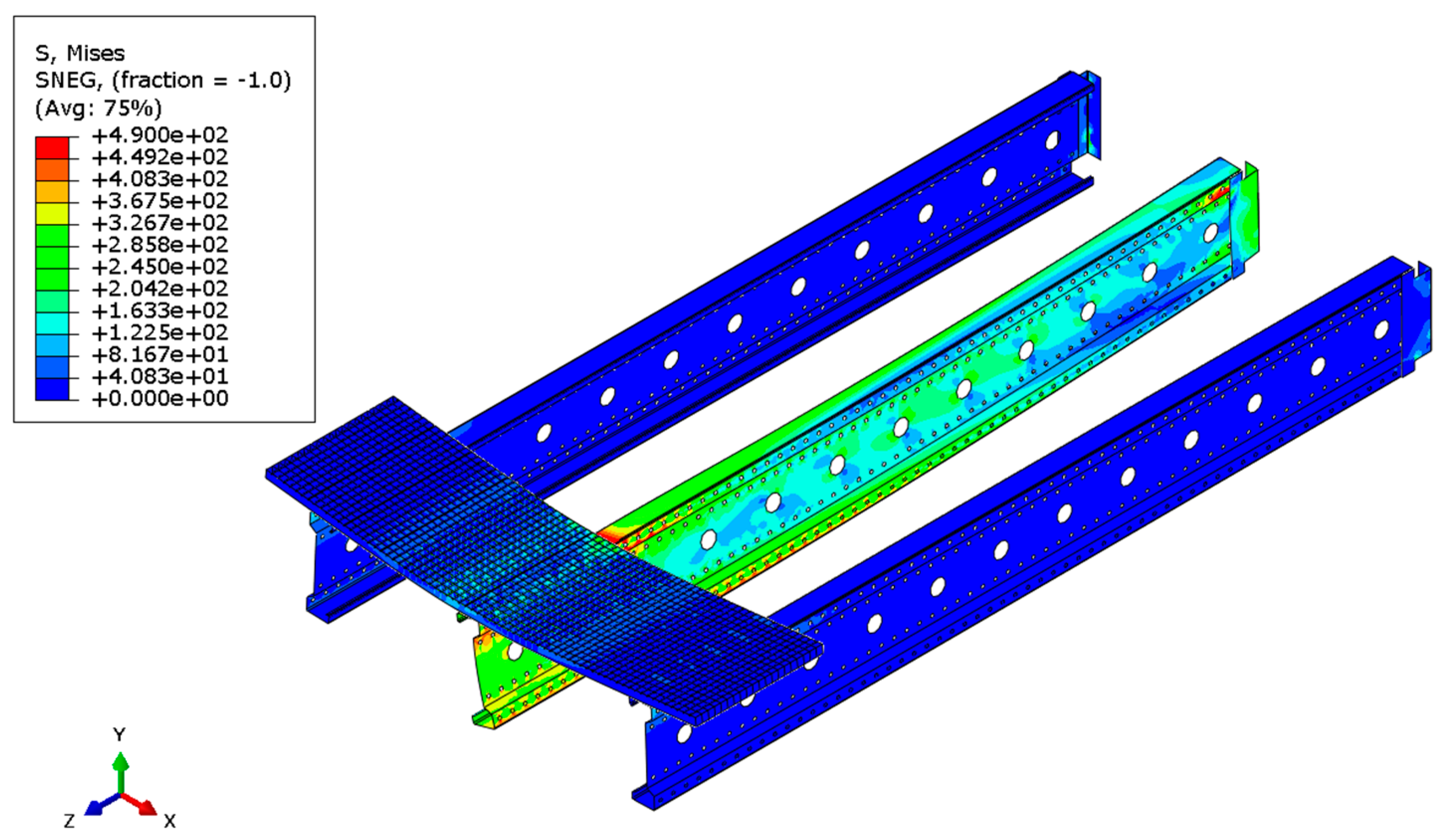
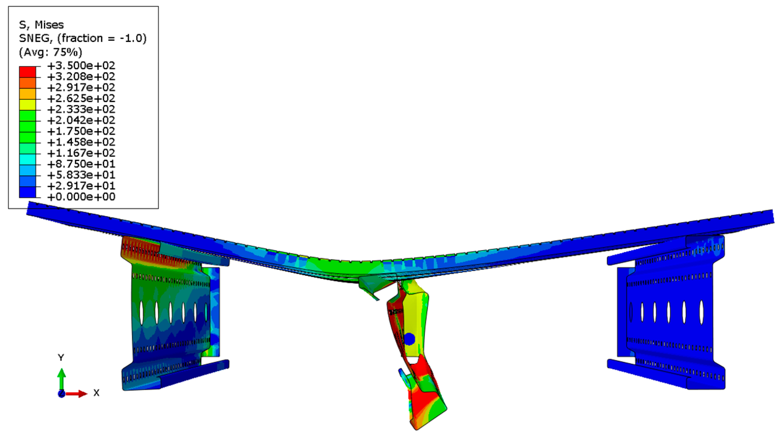
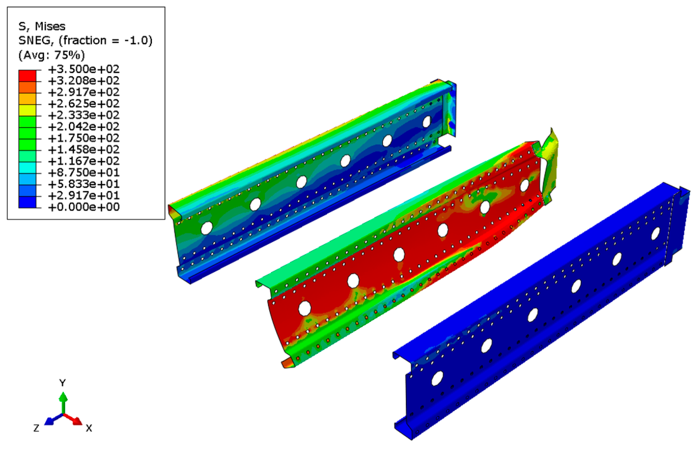
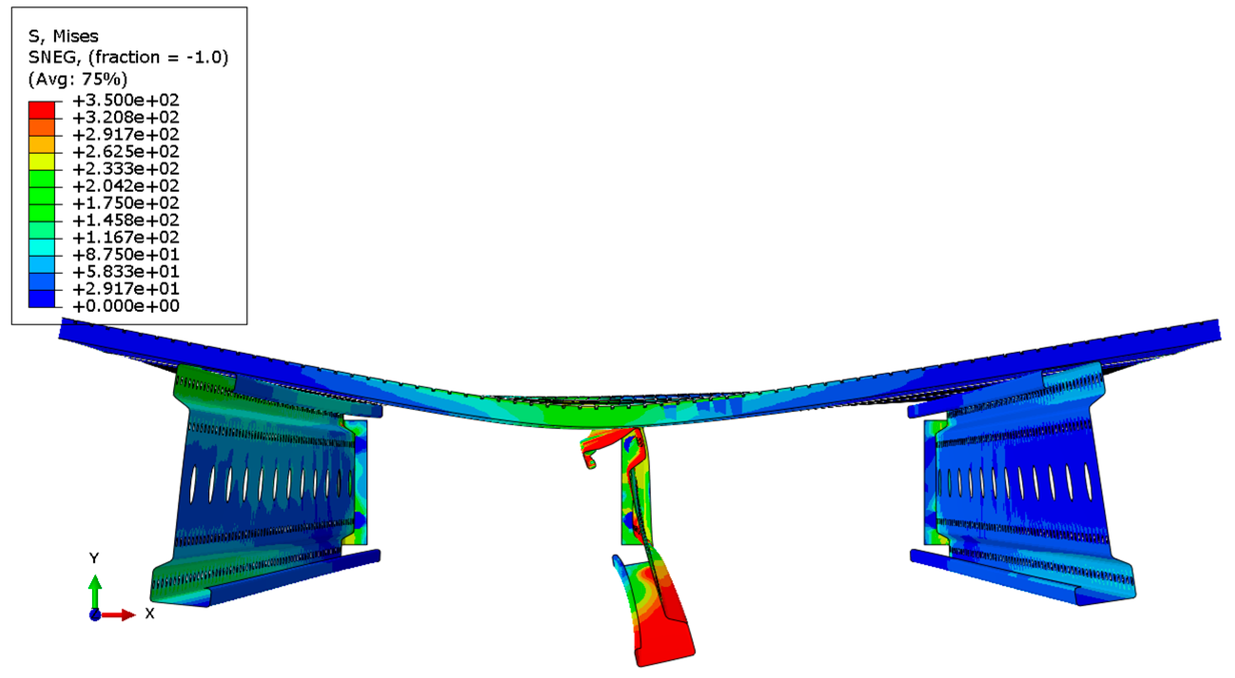
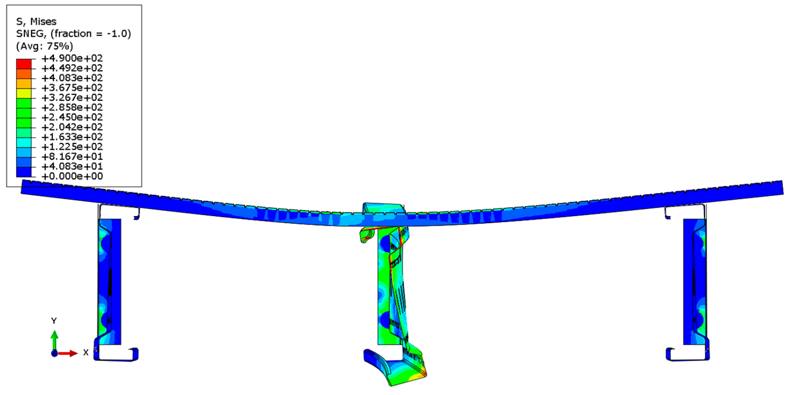
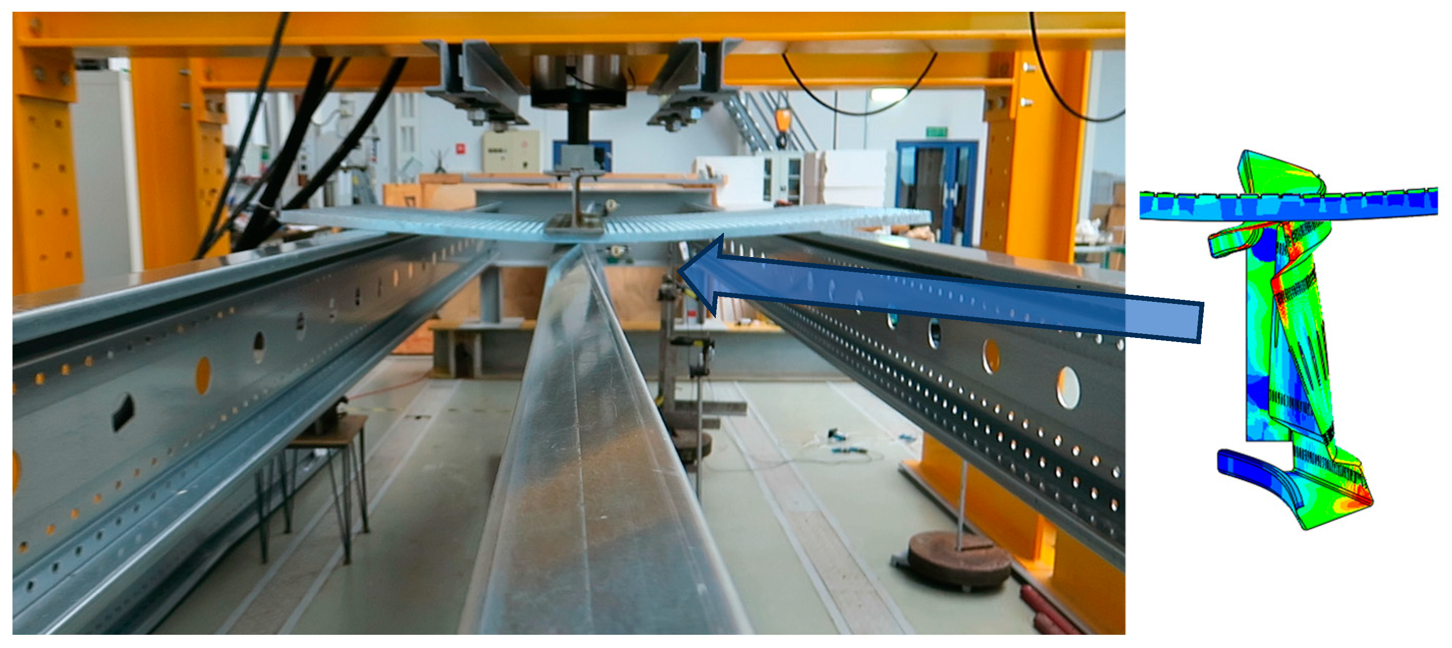
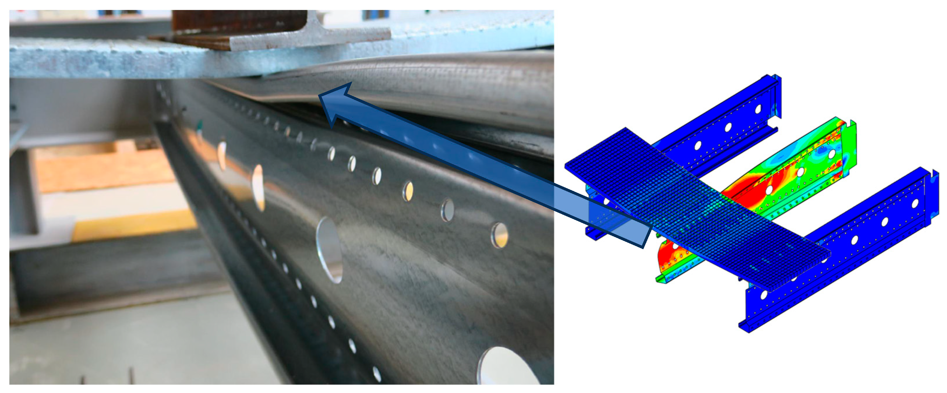
• The study of 6 m beams showed a pattern of destruction through loss of stability, while 3 m beams were destroyed through yielding.
• Numerical simulations and laboratory tests demonstrated analogous destruction patterns.
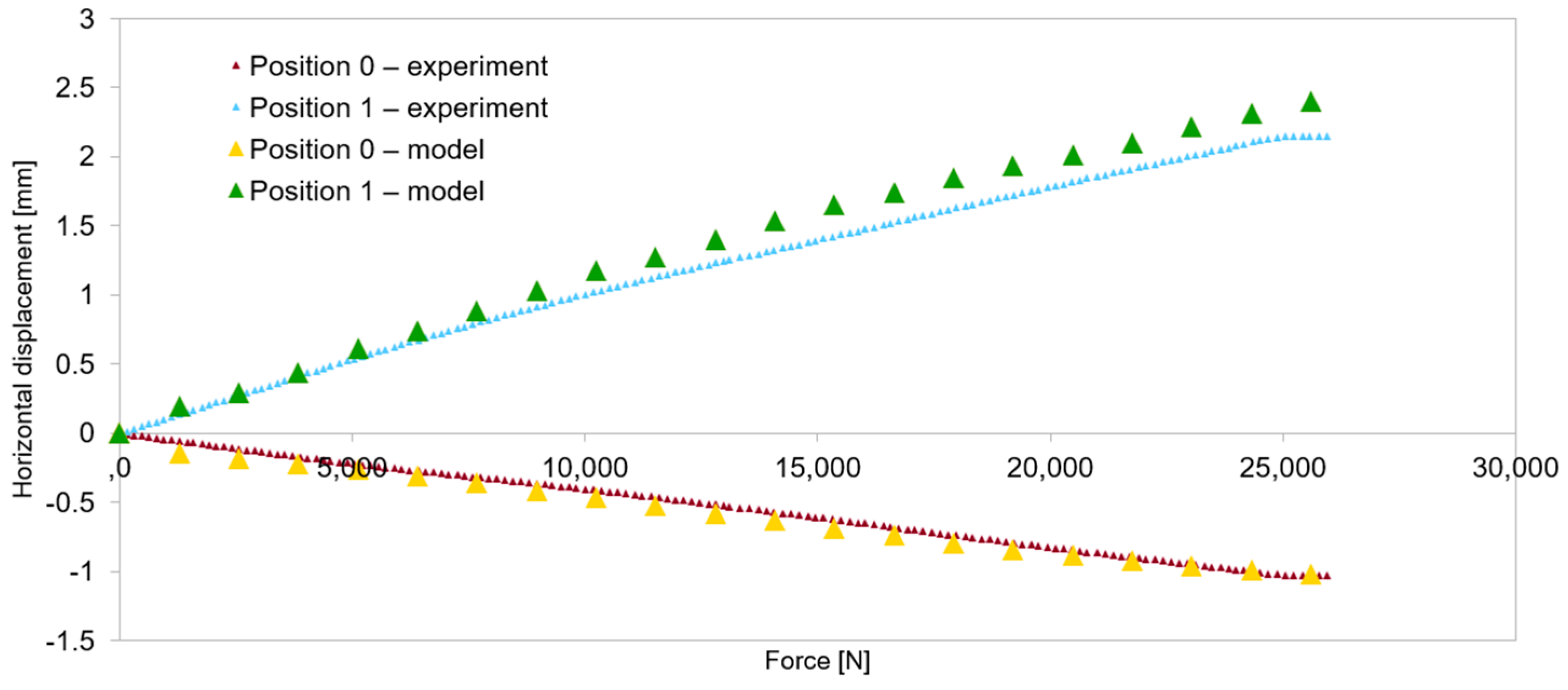
• Measurements of horizontal displacements in all tests showed greater displacements in the lower flange of the beam. This is consistent with expectations, as the upper part of the beam is somewhat “braced” by the bridge deck.
• This observation was also taken into account in the numerical model by applying normal and tangential contact with friction between the bridge deck and beams.
• Based on the conducted tests, it is recommended to place additional bracings between the lower flanges of the beams.
• The connector and the support zone of the beam are the weakest elements of the tested system. Each time, the beam’s destruction process started from the yielding of the connector, which was observed in experimental studies and confirmed in the numerical model for all tested lengths.
• The presented study contributes to a better understanding of the operation of such structural systems.

References

1. Yu, C.; Schafer, B.W. Distortional Buckling Tests on Cold-Formed Steel Members in Bending; Technical Report; Johns Hopkins University: Baltimore, MD, USA, 2005. [Google Scholar]
2. Specification for the Design of Light Gage Steel Structural Members. American Iron and Steel Institute (AISI) Specifications, Standards, Manuals and Research Reports (1946–Present); American Iron and Steel Institute: Washington, DC, USA, 1946. [Google Scholar]
3. EN 1993-1-3:2006; Eurocode 3: Design of Steel Structures—Part 1–3: General Rules-Supplementary Rules for Cold-Formed Members and Sheeting. ECCS: Noordwijk, The Netherlands, 2007. Available online: https://www.phd.eng.br/wp-content/uploads/2015/12/en.1993.1.3.2006.pdf (accessed on 24 November 2023).
4. Landolfo, R. Eurocodes Background and Applications Cold-Formed (CF) Structures. Available online: https://eurocodes.jrc.ec.europa.eu/doc/WS2008/EN1999_8_Landolfo.pdf (accessed on 19 October 2021).
5. Yu, W. Cold-Formed Steel Design; Wiley: Hoboken, NJ, USA, 2000; ISBN 0471-348-090. [Google Scholar]
6. Blandford, G.E.; Louis, S. Current Research on Cold-Formed Steel Structures; International Specialty Conference on Cold-Formed Steel Structures. 1990. Available online: https://scholarsmine.mst.edu/isccss/10iccfss/10iccfss-session7/3 (accessed on 24 November 2023).
7. Lechner, B.; Pircher, M. Analysis of imperfection measurements of structural members. Thin-Walled Struct. 2005, 43, 351–374. [Google Scholar] [CrossRef]
8. Amouzegar, H.; Amirzadeh, B.; Zhao, X.; Schafer, B.; Tootkaboni, M. Statistical analysis of the impact of imperfection modes on collapse behavior of cold-formed steel members. In Proceedings of the Structural Stability Research Council Annual Sta, Nashville, TN, USA, 24–27 March 2015. [Google Scholar]
9. Farzanian, S.; Louhghalam, A.; Schafer, B.W.; Tootkaboni, M. Geometric imperfection models for CFS structural members, Part I: Comparative review of current models. Thin-Walled Struct. 2019. [Google Scholar] [CrossRef]
10. AISI S240-15; North American Standard for Cold Formed Steel Structural Framing. American Iron and Steel Institute: Washington, DC, USA, 2015.
11. GB 50017-2017; Steel Structure Design Standard. China Construction Industry Press Beijing: Beijing, China, 2017.
12. Gonçalves, R.; Dinis, P.B.; Camotim, D. GBT formulation to analyse the first-order and buckling behaviour of thin-walled members with arbitrary cross-sections. Thin-Walled Struct. 2009, 47, 583–600. [Google Scholar] [CrossRef]
13. Gonçalves, R.; Camotim, D. Generalised beam theory-based finite elements for elastoplastic thin-walled metal members. Thin-Walled Struct. 2011, 49, 1237–1245. [Google Scholar] [CrossRef]
14. Abambres, M.; Camotim, D.; Silvestre, N. Modal decomposition of thin-walled member collapse mechanisms. Thin-Walled Struct. 2014, 74, 269–291. [Google Scholar] [CrossRef]
15. Duan, L.; Zhao, J.; Liu, S. A B-splines based nonlinear GBT formulation for elastoplastic analysis of prismatic thin-walled members. Eng. Struct. 2016, 110, 325–346. [Google Scholar] [CrossRef]
16. Hancock, G.J.; Pham, C.H. Buckling analysis of thin-walled sections under localised loading using the semi-analytical finite strip method. Thin-Walled Struct. 2015, 86, 35–46. [Google Scholar] [CrossRef]
17. Ádány, S.; Joó, A.L.; Schafer, B.W. Buckling modes identification of thin-walled members using cFSM base functions. Thin-Walled Struct. 2010, 48, 806–817. [Google Scholar] [CrossRef]
18. Duan, L.; Zhao, J.; Zou, J. Generalized beam theory-based advanced beam finite elements for linear buckling analyses of perforated thin-walled members. Comput. Struct. 2022, 259, 106683. [Google Scholar] [CrossRef]
19. Abaqus Documentation 6.14 (2014); Dassault Systemes Simulia Corp.: Providence, RI, USA, 2014.
Figure 1. Geometry and discretization of the model.
Applsci 14 01505 g001
Figure 2. Method of loading—loading surface.
Applsci 14 01505 g002
Figure 3. Method of loading the model for targeted numerical analyses.
Applsci 14 01505 g003
Figure 4. Static scheme of beams during testing in the elastic range: (a) 3 m beam, (b) 6 m beams, and (c) view of the test station for the 3 m beam.
Applsci 14 01505 g004
Figure 5. Displacement measurement system for horizontal movements during operation in the elastic range.
Applsci 14 01505 g005
Figure 6. Material sample with an extensometer during testing.
Applsci 14 01505 g006
Figure 18. Distribution of reduced Mises stresses and deformation of the system with a span of 3 m.
Applsci 14 01505 g018
Figure 19. Distribution of reduced Mises stresses and deformation of the system with a span of 3 m—cross-section.
Applsci 14 01505 g019
Figure 20. Distribution of reduced Mises stresses and deformation of the system with a span of 3 m—view without the bridge deck.
Applsci 14 01505 g020
Figure 21. Distribution of reduced Mises stresses and deformation of the system with a span of 6 m.
Applsci 14 01505 g021
Figure 22. Distribution of reduced Mises stresses and deformation of the system with a span of 6 m—cross-section.
Applsci 14 01505 g022
Figure 23. Distribution of reduced Mises stresses and deformation of the system with a span of 6 m—view without the bridge deck.
Applsci 14 01505 g023
Figure 24. Load-bearing curves developed based on simulations of structural systems with spans ranging from 3 m to 6 m.
Applsci 14 01505 g024