An Improved Adaptive Iterative Extended Kalman Filter Based on Variational Bayesian

Abstract

The presence of unknown heavy-tailed noise can lead to inaccuracies in measurements and processes, resulting in instability in nonlinear systems. Various estimation methods for heavy-tailed noise exist. However, these methods often trade estimation accuracy for algorithm complexity and parameter sensitivity. To tackle this challenge, we introduced an improved variational Bayesian (VB)-based adaptive iterative extended Kalman filter. In this VB framework, the inverse Wishart distributionis used as the prior for the state prediction covariance matrix. The system state and noise parameter posterior distributions are then iteratively updated for adaptive estimation. Furthermore, we make adaptive adjustments to the IEKF filter parameters to enhance sensitivity and filtering accuracy, thus ensuring robust prediction estimation. A two-dimensional target tracking and nonlinear numerical UNGM simulation validated our algorithm. Compared to existing algorithms RKF-ML and GA-VB, our method showed significant improvements in $RMS{E}_{\mathrm{pos}}$ and $RMS{E}_{\mathrm{vel}}$, with increases of 21.81% and 22.11% respectively, and a 49.04% faster convergence speed. These results highlight the method’s reliability and adaptability.

1. Introduction

Given the extensive use of nonlinear systems [1,2] in various domains, including radar [3,4], communication [5,6], navigation [7,8], control [9,10], finance [11], and statistics [12,13], the nonlinear dynamics of these systems require sophisticated filtering techniques for robust and precise estimation [14,15]. However, the effectiveness of these filtering techniques significantly diminishes in the presence of heavy-tailed noise and errors. According to previous research [16,17], this leads to a marked decline in estimation accuracy.

Numerous filters have been proposed to address the issue of heavy-tailed noise impacting system tracking. Notable among these are the robust variational Bayesian filter [18,19,20], Student’s t-based filters (RSTFs) [21,22], Huber’s M-estimation-based filters [23,24], and the maximum correlation entropy-based filters [25]. While these filters demonstrate enhanced tracking performance and effectively mitigate the negative impact of heavy-tailed noise, they face challenges in precise parameter selection and computational complexity. The need for accurate parameter calibration, a potentially time-consuming and obstructive task, combined with the computational demands of these methods, may limit their practical applicability in real-time scenarios. Consequently, there is an urgent need to improve and streamline the parameter selection process, thereby reducing computational complexity.

As a key technique in nonlinear recursive filtering, the Extended Kalman Filter (EKF) is widely recognized and utilized [16,26,27]. Its popularity stems from several advantages, such as obviating the need for calculating nominal trajectories, its straightforward methodology, and ease of implementation. However, enhancing the functionality and effectiveness of state estimation filters in real-world applications remains crucial. The Kalman filter algorithm based on Huber [28,29], for example, shows resilience to outliers and superior performance in non-Gaussian settings. Yet, it faces increased computational complexity, requires fine-tuning of parameters, and may be less efficient in Gaussian environments. The Interactive Multiple Model (IMM)-based Kalman filter [30,31] offers improved estimation accuracy and robustness amidst model uncertainties, but this benefit comes with increased computational and implementation complexities, as well as reliance on precise model selection and meticulous parameter tuning. A robust Gaussian approximate filter, integrating unknown scale matrices and degrees of freedom parameters, was introduced in the literature (GA-VB) [32]. To enhance this algorithm, the variational Bayesian (VB) method was employed to modify the state and posterior probability density functions (PDFs) for each parameter individually, aiming to reduce the overall complexity while inadvertently increasing sensitivity to parameters. Concurrently, literature (RKF-ML) [33] presented a robust state estimation algorithm using the maximum likelihood (ML) distribution to model heavy-tailed noise. This method notably avoids the need for manually selecting the degrees of freedom (DOF) parameters, thus being less sensitive to free parameters. However, it requires a VB approach to adaptively estimate ML distribution parameters in a closed recursive state, adding to the overall complexity. These algorithms underscore the trade-offs between complexity and sensitivity in algorithm design, highlighting the necessity for a nuanced approach that carefully balances these factors to achieve optimal performance in state estimation algorithms under challenging conditions.

Addressing parameter sensitivity and algorithmic complexity, this paper introduces a new approach: an improved variational Bayesian (VB)-based adaptive iterative extended Kalman filter (VBAIEKF). This method aims to enhance the accuracy of filters handling imprecise heavy-tailed noise while simultaneously addressing parameter sensitivity and reducing algorithmic complexity. Initially, the inverse Wishart (IW) distribution is utilized to model inaccurate measurement noise, treating the system state and measurement noise covariance as parameters to be estimated. To estimate these parameters, the variational Bayesian (VB) method computes the joint posterior probability density functions (PDFs) for these parameters, thereby accomplishing the state estimation of the system. This approach effectively addresses variability in both noise and prediction error covariances. The algorithm exhibits the following highlights:

(1) The approach is characterized by a notable insensitivity to its parameters, possessing the ability to withstand variations in parameter values.

(2) The approach exhibits lower computational complexity, rendering it suitable for real-time applications.

(3) This approach exhibits significant adaptability and reliability when confronted with an uncertain environment.

The algorithm proposed in this article adeptly addresses the challenge of concurrently managing noise fluctuations and prediction error covariance in the state estimation process. When compared with two optimized algorithms, GA-VB [32] and RKF-ML [33], the performance of the VBAIEKF is notably impressive. Characterized by low sensitivity to parameters, minimal complexity, excellent convergence, and adaptability, these attributes render it a particularly promising solution for achieving precise state estimation in scenarios with heavy-tailed noise.

The primary framework is outlined as follows. Section 2 delineates the procedural workflow of the VBAIEKF algorithm, where we deduce the filter and emphasize its unique characteristics. In Section 3, we conduct a thorough comparison between the proposed VBAIEKF and the GA-VB [32] and RKF-ML [33] algorithms. This comparison focuses on two-dimensional target tracking with nonlinear uncertain heavy-tailed noise and nonlinear numerical UNGM. The comparative analysis clearly demonstrates the superior performance of the VBAIEKF. Section 4 provides definitive remarks that summarize the findings and implications of the study.

2. Computational Procedure

2.1. System Model

Consider the following noisy nonlinear system shown by the state space model:

$$x_t=f_{t-1}\left(x_{t-1}\right)+w_{t-1}$$

(1)

$$z_t=h_t\left(x_t\right)+v_t$$

(2)

where $x_t\in {\mathbb{R}}^n$ is an observable yet unmeasurable state vector, $z_t={\mathbb{R}}^m$ is a vector of measurements that may be observed, $f_{t-1}(·)$ and $h_t(·)$ are recognized nonlinear functions. To simplify computations and ensure the convergence of the Taylor series expansion, assume that $f_{t-1}(·)$ and $h_t(·)$ are, without loss of generality, analytic functions that are sufficiently smooth and differentiable. The covariance matrices of the random variables $w_{t-1}$ and $v_t$ are denoted as $Q_t$ and $R_t$, respectively. The process noise $w_{t-1}$ is a Gaussian process with a mean of zero and an unknown covariance matrix $Q_t$. The measurement noise, denoted as $v_t$, is a type of Gaussian white noise with a mean of zero. The covariance matrix $R_t$ associated with this noise is unknown. First, a Taylor Series expansion (TSE) [34], which can be stated as the following, is used to linearize locally the nonlinear functions $f_{t-1}(·)$ and $h_t(·)$:

$$\begin{array}{c}\hfill \begin{array}{ccc}\hfill f\left(x_{t-1}\right)& =f\left({\widehat{x}}_{t-1}\right)+{\left.\frac{\partial f\left(x_{t-1}\right)}{\partial x_{k-1}}\right|}_{x_{t-1}={\widehat{x}}_{t-1}}\hfill & \times \left(x_{t-1}-{\widehat{x}}_{t-1}\right)+H.O.T\\ & \approx f\left({\widehat{x}}_{t-1}\right)+F_t{\tilde{x}}_{t-1}\hfill \end{array}\end{array}$$

(3)

$$\begin{array}{c}\hfill \begin{array}{ccc}\hfill h\left(x_t\right)& =h\left({\widehat{x}}_{t\mid t-1}\right)+{\left.\frac{\partial \mathrm{h}\left(x_t\right)}{\partial x_t}\right|}_{x_{t-1}={\widehat{x}}_{t\mid t-1}}\hfill & \times \left(x_t-{\widehat{x}}_{t\mid t-1}\right)+H.O.T\\ & \approx h\left({\widehat{x}}_{t\mid t-1}\right)+H_t{\tilde{x}}_{t\mid t-1}\hfill \end{array}\end{array}$$

(4)

The requirement for bounded higher-order terms (H.O.T) is crucial to guarantee the convergence and accuracy of the Taylor series expansion. Following the application of the Taylor series expansion, the nonlinear functions $f_{t-1}(·)$ and $h_t(·)$ are approximated by linear functions with error terms $F_t$ and $H_t$, respectively.

When there is heavy-tailed noise, the covariance matrix of the process and measurement noise is usually imprecise. To resolve this problem, one can utilize a variational Bayesian (VB) method [19,35,36], and subsequently apply an iterative extended Kalman filter to estimate the state vector $x_t$. This work presents an improved variational Bayesian iterative extended Kalman filtering (VBAIEKF) technique designed for tracking estimation.

2.2. Prior Distributions

Provide a detailed description of the updating process for prior distributions.

In the Kalman filtering paradigm, the likelihood probability density function (PDF) $p\left(\widetilde{{\mathrm{Z}}_{\mathrm{t}}}\mid \widetilde{{\mathrm{X}}_{\mathrm{t}}}\right)$ and the one-step anticipated PDF $p\left(\widetilde{{\mathrm{X}}_{\mathrm{t}}}\mid {\tilde{\mathrm{Z}}}_{1:t-1}\right)$ are Gaussian distributions:

$$\begin{array}{c}p\left(\widetilde{{\mathrm{X}}_{\mathrm{t}}}\mid {\tilde{\mathrm{Z}}}_{1:t-1}\right)=N\left(\widetilde{{\mathrm{X}}_{\mathrm{t}}};{\widehat{X}}_{t\mid t-1},P_{t\mid t-1}\right)\end{array}$$

(5)

$$\begin{array}{c}p\left({\tilde{\mathrm{Z}}}_t\mid \widetilde{{\mathrm{X}}_{\mathrm{t}}}\right)=N\left({\tilde{\mathrm{Z}}}_t;h\left(\widetilde{{\mathrm{X}}_{\mathrm{t}}}\right),R_t\right)\end{array}$$

(6)

where the Gaussian distribution $\tilde{\mathrm{N}}(A;\alpha ,\sigma )$ has the following mean and variance: $\alpha$, $\sigma$, and its PDF is:

$$\begin{array}{c}\hfill \tilde{\mathrm{N}}(A;\alpha ,\sigma )=\frac{1}{\sqrt{\left|2\pi \sigma \right|}}{e}^{-\frac{1}{2}{(A-\alpha )}^T{\sigma }^{-1}(A-\alpha )}\end{array}$$

(7)

The anticipated state vector ${\widehat{X}}_{t\mid t-1}$ and the related one-step predicted covariance matrix $P_{t\mid t-1}$ can be represented as follows:

$$\begin{array}{c}{\widehat{X}}_{t\mid t-1}=F{\widehat{X}}_{t-1\mid t-1}+{\mu }_t\end{array}$$

(8)

$$\begin{array}{c}{P}_{t\mid t-1}=F{P}_{t-1\mid t-1}{F}^T+Q_{t-1}\end{array}$$

(9)

where ${\widehat{X}}_{t-1\mid t-1}$ and $P_{t-1\mid t-1}$ denote the state estimate and estimation error covariance matrix at time $t-1$, respectively. Where ${\widehat{X}}_{t-1\mid t-1}$ and $P_{t-1\mid t-1}$ represent the state estimation and the covariance matrix of the estimate error at time $t-1$, respectively. The coefficient $P_{t\mid t-1}$ in Equation (9) is imprecise, and the actual process noise covariance matrix $Q_t$ is not known.

The inverse Wishart (IW) distribution is considered the conjugate prior distribution for a Gaussian distribution with a specified mean covariance matrix in Bayesian statistics. Variational Bayesian (VB) approaches offer a closed-form analytical solution to this intricate problem. Let us consider the Wishart distribution $W\left({\phi }^{-1};\beta ,\theta -1\right)$, where ${\phi }^{-1}$ is the inverse matrix of a positive definite matrix $\phi$. The matrix $\phi$ is distributed according to the inverse Wishart (IW) distribution [37].

$$\begin{array}{c}IW(\phi ;\beta ,\theta )=\frac{{\left|\theta \right|}^{\beta /2}{\left|\phi \right|}^{-(\beta +d+1)/2}{\mathrm{e}}^{-tr\left({{\theta }_B}^{-1}\right)/2}}{2^{d\beta /2}{\mathrm{\Gamma }}_d(\beta /2)}\end{array}$$

(10)

where $\beta >d+1$ represents the degree of freedom, $\theta$ represents a $d\times d$ positive definite matrix, $\mathrm{d}$ represents the dimension of $\theta ,{\mathrm{\Gamma }}_d(·)$ represents the multivariate gamma distribution, and trace $(·)$ represents the trace function. The expected value of the matrix $\phi \sim IW(\phi ;\beta ,\theta )$, if it follows the IW distribution, is $E\left(\phi \right)=\frac{\theta }{\beta -d-1}$. Due to the fact that $P_{t\mid t-1}$ and $R_t$ are the normal PDF covariance matrices, $p\left(P_{t\mid t-1}\mid {\tilde{\mathrm{Z}}}_{1:t-1}\right)$ and $p\left(R_t\mid {\tilde{\mathrm{Z}}}_{1:t-1}\right)$ can be written as IW distributions:

$$\begin{array}{c}p\left(P_{t\mid t-1}\mid {\tilde{\mathrm{Z}}}_{1:t-1}\right)=IW\left(P_{t\mid t-1};{\widehat{t}}_{t\mid t-1},{\widehat{T}}_{t\mid t-1}\right)\end{array}$$

(11)

$$\begin{array}{c}p\left(R_t\mid {\tilde{\mathrm{Z}}}_{1:t-1}\right)=IW\left(R_{t\mid t-1};{\widehat{u}}_{t\mid t-1},{\widehat{U}}_{t\mid t-1}\right)\end{array}$$

(12)

where ${\widehat{u}}_{t\mid t-1}$ and ${\widehat{U}}_{t\mid t-1}$ denote the degrees of freedom and scale matrices of $p\left(R_t\mid {\tilde{\mathrm{Z}}}_{1:t-1}\right)$, respectively, ${\widehat{t}}_{t\mid t-1}$ and ${\widehat{T}}_{t\mid t-1}$ denote the degrees of freedom and scale matrices of $p\left(P_{t\mid t-1}\mid \right.$$\left.{\tilde{\mathrm{Z}}}_{1:t-1}\right)$. Then, it is necessary to determine the values of ${\widehat{t}}_{t\mid t-1},{\widehat{T}}_{t\mid t-1},{\widehat{u}}_{t\mid t-1}$ and ${\widehat{U}}_{t\mid t-1}$.

The nominal error covariance matrix $P_{t\mid t-1}$ can be set equal to the mean of matrix ${\overline{P}}_{t\mid t-1}$.

Using $E\left(\phi \right)=\frac{\theta }{\beta -d-1}$, we arrive at the following:

$$\begin{array}{c}\frac{{\widehat{T}}_{t\mid t-1}}{{\widehat{T}}_{t\mid t-1}-n-1}={\overline{P}}_{t\mid t-1}=F{P}_{t-1\mid t-1}{F}^T+{\overline{Q}}_{t-1}\end{array}$$

(13)

where n stands for the dimension of the state $T_{t\mid t-1}$, and ${\overline{Q}}_{t-1}$ stands for the nominal process noise covariance. Let:

$$\begin{array}{c}{\widehat{t}}_{t\mid t-1}=a+\tau +1\end{array}$$

(14)

where $T\ge 0$ is the correction factor. The outcome of entering Equation (14) into (13) is:

$$\begin{array}{c}{\overline{T}}_{t\mid t=1}=\tau {\overline{P}}_{t\mid t-1}\end{array}$$

(15)

The prior probability density function (PDF) distribution $p\left(R_{t-1}\mid {\tilde{\mathrm{Z}}}_{1:t-1}\right)$ of the measurement noise covariance matrix $R_{t-1}$ is influenced by the inverse Wishart (IW) distribution. Similarly, the posterior PDF distribution $p\left(R_{t-1}\mid {\tilde{\mathrm{Z}}}_{1:t-1}\right)$ of this matrix should also follow an IW distribution, as stated in Equation (12):

$$\begin{array}{c}p\left(R_{t-1}\mid {\tilde{\mathrm{Z}}}_{1:t-1}\right)=IW\left(R_{t-1};{\widehat{u}}_{t-1\mid t-1},{\widehat{U}}_{t-1\mid t-1}\right)\end{array}$$

(16)

It is unknown what the dynamic model of the noise variance in Equation (17) appears like in real-world applications: $p\left(R_t\mid R_{t-1}\right)$. To preserve and propagate the approximate posterior at the prior moment, we select the forgetting factor $\rho$ and formulate the prior parameters as follows:

$$\begin{array}{c}{\widehat{u}}_{k\mid t-1}=\rho \left({\widehat{u}}_{t-1\mid t-1}-b-1\right)+b+1\end{array}$$

(17)

$$\begin{array}{c}{\widehat{U}}_{t\mid t-1}=\rho {\widehat{U}}_{t-1\mid t-1}\end{array}$$

(18)

The forgetting factor $\rho$ reflects the degree of temporal variation, which ranges from 0 to 1, inclusive. A value of $\rho =1$ indicates the variance at a steady state, with lower values of $\rho$ corresponding to higher frequencies of variations throughout time.

2.3. Posterior PDFs

Here, we elaborate on the meticulous process of updating posterior PDFs.

In order to calculate ${\tilde{\mathrm{X}}}_t$, $P_{t\mid t-1}$, and $R_t$, the joint posterior probability density function $p\left({\tilde{\mathrm{X}}}_t,P_{t\mid t-1},R_t\mid {\tilde{\mathrm{Z}}}_{1:t}\right)$ needs to be determined. Since there is no analytical solution available for this joint posterior probability density function (PDF), the variational Bayesian (VB) approach is employed to derive an approximate PDF that is factorized and flexible for:

$$\begin{array}{c}p\left({\tilde{\mathrm{X}}}_t,P_{t\mid t-1},R_t\mid {\tilde{\mathrm{Z}}}_{1:t}\right)\approx q\left({\tilde{\mathrm{X}}}_t\right)q\left(P_{t\mid t-1}\right)q\left(R_t\right)\end{array}$$

(19)

where $q(·)$ corresponds to the somewhat posterior PDF of $p(·)$. Therefore, it is possible to produce the VB approximation by minimizing the Kullback–Leibler Divergence (KLD) [38] between the posterior PDFs of the genuine joint $p\left({\tilde{\mathrm{X}}}_t,P_{t\mid t-1},R_t\mid {\tilde{\mathrm{Z}}}_{1:t}\right)$ and the approximation $q\left({\tilde{\mathrm{X}}}_t\right),q\left(P_{t\mid t-1}\right),q\left(R_t\right)$:

$$\begin{array}{c}\left\{q\left({\tilde{\mathrm{X}}}_t\right),\left(P_{t|t-1}\right),q\left(R_t\right)\right\}=argminKLD\left(\begin{array}{c}q\left({\tilde{\mathrm{X}}}_t\right),q\left(P_{t\mid t-1}\right)q\left(R_t\right)\hfill \\ \Vert p\left({\tilde{\mathrm{X}}}_t,P_{t|t-1},R_t\mid {\tilde{\mathrm{Z}}}_{1:t}\right)\hfill \end{array}\right)\hfill \end{array}$$

(20)

Therefore, it can also be written as:

$$\begin{array}{c}\hfill \begin{array}{c}log{q}^{(i+1)}\left(P_{t\mid t-1}\right)=-\frac{1}{2}\left(a+{\widehat{t}}_{t\mid t-1}+2\right)log\left|P_{t\mid t-1}\right|-\frac{1}{2}tr\left(\left({\tilde{\mathrm{A}}}_t^{\left(i\right)}+T_{t\mid t-1}\right)P_{t\mid t-1}^{-1}\right)+c_{P_{t\mid t-1}}\hfill \end{array}\end{array}$$

(21)

Additionally, Equations (22) and (27) can be obtained. $q^{(i+1)}(·)$ represents the approximate PDF of the $i+1$th iteration of $q(·)$, and ${\tilde{\mathrm{A}}}_t^{\left(i\right)}$ is defined as follows:

$$\begin{array}{c}\hfill \begin{array}{c}{\tilde{\mathrm{A}}}_t^{\left(i\right)}={\mathrm{E}}^{\left(i\right)}\left[\left({\tilde{\mathrm{X}}}_t-{\widehat{X}}_{t\mid t-1}\right){\left({\tilde{\mathrm{X}}}_t-{\widehat{X}}_{t\mid t-1}\right)}^T\right]\hfill \\ =P_{t\mid t}^{\left(i\right)}+\left({\widehat{X}}_{t\mid t}^{\left(i\right)}-{\widehat{X}}_{t\mid t-1}\right){\left({\widehat{X}}_{t\mid t}^{\left(i\right)}-{\widehat{X}}_{t\mid t-1}\right)}^T\hfill \end{array}\end{array}$$

(22)

where ${\mathrm{E}}^{\left(i\right)}\left[\rho \right]$ represents the expected value of variable $\rho$ at iteration i-th.

The IW distribution with the parameter of freedom ${\widehat{t}}_{t\mid t-1}^{(i+1)}$ and scale matrix ${\widehat{T}}_{t\mid t-1}^{(i+1)}$ can be regarded as $q^{(i+1)}\left(P_{t\mid t-1}\right)$:

$$q^{(i+1)}\left(P_{t\mid t-1}\right)=IW\left(P_{t\mid t-1},{\widehat{t}}_t^{(i+1)},{\widehat{T}}_t^{(i+1)}\right)$$

(23)

where ${\widehat{t}}_{t\mid t-1}^{(i+1)}$ is the parameter of freedom and ${\widehat{T}}_{\mathrm{t}\mid \widehat{t}-1}^{(i+1)}$ is the scale matrix:

$$\begin{array}{c}{\widehat{t}}_t^{(i+1)}={\widehat{t}}_{t\mid t-1}+1\end{array}$$

(24)

$$\begin{array}{c}{\widehat{T}}_t^{(i+1)}={\tilde{\mathrm{A}}}_t^{\left(i\right)}+{\widehat{T}}_{t\mid t-1}\end{array}$$

(25)

Its comprehensive form is:

$$\begin{array}{c}\hfill \begin{array}{c}log{q}^{(i+1)}\left(R_t\right)=-\frac{1}{2}\left(b+{\widehat{u}}_{t\mid t-1}+2\right)log\left|R_t\right|-\frac{1}{2}tr\left(\left({\tilde{\mathrm{Z}}}_t^{\left(i\right)}+{\widehat{U}}_{t\mid t-1}\right)R_t^{-1}\right)+c_{R_t}\hfill \end{array}\end{array}$$

(26)

where $B_{\mathrm{k}}^{\left(i\right)}$ has the following definition:

$$\begin{array}{c}\hfill \begin{array}{c}{\tilde{\mathrm{B}}}_k^{\left(i\right)}=E^i\left[\left({\tilde{\mathrm{Z}}}_t-h\left({\tilde{\mathrm{X}}}_t\right)\right){\left({\tilde{\mathrm{Z}}}_t-h\left({\tilde{\mathrm{X}}}_t\right)\right)}^T\right]\hfill \\ =\int \left({\tilde{\mathrm{Z}}}_t-h\left({\tilde{\mathrm{X}}}_t\right)\right){\left({\tilde{\mathrm{Z}}}_t-h\left({\tilde{\mathrm{X}}}_t\right)\right)}^{T}N\left({\tilde{\mathrm{X}}}_t;{\widehat{X}}_{t\mid t}^{\left(i\right)}{P}_{t\mid t}^{\left(i\right)}\right)d{\tilde{\mathrm{X}}}_t\hfill \end{array}\end{array}$$

(27)

Equation (26) states that $q^{(i+1)}\left(R_t\right)$ may be thought of as the IW distribution, where ${\widehat{u}}_{t\mid t-1}^{(i+1)}$ stands in for the freedom parameter and ${\widehat{U}}_{t\mid t-1}^{(i+1)}$ for the scale matrix.

$$\begin{array}{c}{q}^{(i+1)}\left(R_t\right)=IW\left(R_t;{\widehat{u}}_t^{(i+1)},{\widehat{U}}_t^{(i+1)}\right)\end{array}$$

(28)

When the scale matrix ${\widehat{U}}_{t\mid t-1}^{(i+1)}$ and the freedom parameter ${\widehat{u}}_{t\mid t-1}^{(i+1)}$ are represented as:

$$\begin{array}{c}{\widehat{u}}_t^{(i+1)}={\widehat{u}}_{t\mid t-1}+1\end{array}$$

(29)

$$\begin{array}{c}{\widehat{U}}_t^{(i+1)}={\tilde{\mathrm{B}}}_t^{\left(i\right)}+{\widehat{U}}_{t\mid t-1}\end{array}$$

(30)

where can be represented as:

$$\begin{array}{c}{E}^{(i+1)}\left[R_t^{-1}\right]=\left({\widehat{u}}_t^{(i+1)}-b-1\right){\left({\widehat{U}}_t^{(i+1)}\right)}^{-1}\end{array}$$

(31)

$$\begin{array}{c}{E}^{(i+1)}\left[P_{t\mid t-1}^{-1}\right]=\left({\widehat{t}}_t^{(i+1)}-a-1\right){\left({\widehat{T}}_t^{(i+1)}\right)}^{-1}\end{array}$$

(32)

After the $i+1$th iteration update, the one-step predicted PDF and likelihood PDF may be described by the following equations:

$$\begin{array}{c}{p}^{(i+1)}\left({\tilde{\mathrm{X}}}_t\mid {\tilde{\mathrm{Z}}}_{1:t-1}\right)=N\left({\tilde{\mathrm{X}}}_t;{\widehat{X}}_{t\mid t-1},{\widehat{P}}_{t\mid t-1}^{(i+1)}\right)\end{array}$$

(33)

$$\begin{array}{c}{p}^{(i+1)}\left({\tilde{\mathrm{Z}}}_t\mid {\tilde{\mathrm{X}}}_t\right)=N\left({\tilde{\mathrm{Z}}}_t;h\left({\tilde{\mathrm{X}}}_t\right),{\widehat{R}}_t^{(i+1)}\right)\end{array}$$

(34)

Following are the formulations for the matrix ${\widehat{P}}_{t\mid t-1}^{(i+1)}$ of the corrected predicted error covariance and matrix ${\widehat{R}}_t^{(i+1)}$ of the measured noise covariance:

$$\begin{array}{c}{\widehat{P}}_{t\mid t-1}^{(i+1)}={\left\{E^{(i+1)}\left[P_{t\mid t-1}^{-1}\right]\right\}}^{-1}\end{array}$$

(35)

$$\begin{array}{c}{\widehat{R}}_t^{(i+1)}={\left\{E^{(i+1)}\left[R_t^{-1}\right]\right\}}^{-1}\end{array}$$

(36)

Equations (33)–(36) can be transformed into a Gaussian distribution with a mean of ${\tilde{\mathrm{X}}}_{t\mid t}^{(i+1)}$ and a variance of $P_{t\mid t}^{(i+1)}$ by considering the following:

$$\begin{array}{c}{q}^{(i+1)}\left({\tilde{\mathrm{X}}}_t\right)=N\left({\tilde{\mathrm{X}}}_t;{\tilde{\mathrm{X}}}_{t\mid t}^{(i+1)},P_{t\mid t}^{(i+1)}\right)\end{array}$$

(37)

The predicted value ${\tilde{\mathrm{X}}}_{t\mid t}^{(i+1)}$ and prediction error covariance $P_{t\mid t}^{(i+1)}$ are then calculated using IEKF at the $i+1$th iteration as follows:

$$\begin{array}{c}{K}_t^{(i+1)}={\widehat{P}}_{t\mid t-1}^{(i+1)}{H}_t^{\top }{\left(H_t{\widehat{P}}_{t\mid t-1}^{(i+1)}{H}_t^T+{\widehat{R}}_t^{(i+1)}\right)}^{-1}\end{array}$$

(38)

$$\begin{array}{c}{\widehat{X}}_t^{(i+1)}={\widehat{X}}_{t\mid t-1}+K_t^{(i+1)}\left({\tilde{\mathrm{Z}}}_t-h\left({\widehat{X}}_{t\mid t-1}\right)\right)\end{array}$$

(39)

$$\begin{array}{c}{\widehat{P}}_{t\mid t}^{(i+1)}={\widehat{P}}_{t\mid t-1}^{(i+1)}-K_t^{(i+1)}{H}_t{\widehat{P}}_{t\mid t-1}^{(i+1)}\end{array}$$

(40)

Repeat Equations (38)–(40) until the threshold for the condition Euclidean norm

$∥{\tilde{\mathrm{X}}}_t^{(i+1)}-{\widehat{X}}_t^{\left(i\right)}∥⩽\epsilon ,\epsilon$ is reached. The following expressions provide variational approximations of posterior PDFs after N iterations:

$$\begin{array}{c}\hfill \begin{array}{c}{\tilde{\mathrm{X}}}_t=\left({\tilde{\mathrm{X}}}_t;{\widehat{X}}_{t\mid t},P_{t\mid t}\right)\hfill \end{array}\end{array}$$

(41)

$$\begin{array}{c}\hfill \begin{array}{c}q\left(P_{t\mid t-1}\right)=IW\left(P_{t\mid t-1};{\widehat{t}}_{t\mid t},{\widehat{T}}_{t\mid t}\right)\hfill \end{array}\end{array}$$

(42)

$$\begin{array}{c}\hfill \begin{array}{c}q\left(R_t\right)=IW\left(P_{t\mid t-1};{\widehat{u}}_{t\mid t},{\widehat{U}}_{t\mid t}\right)\hfill \end{array}\end{array}$$

(43)

2.4. Algorithm 1

The recursive operation of the improved adaptive iterative extended Kalman filter based on variational Bayesian (VBAIEKF) is depicted in the pseudocode in Algorithm 1.

Algorithm 1 One time step of the proposed VBAIEKF

Input: ${\widehat{X}}_{t-1\mid t-1},P_{k-1\mid k-1},{\widehat{u}}_{t-1\mid t-1},{\widehat{U}}_{t-1\mid t-1},F,h\left({\tilde{\mathrm{X}}}_t\right),{\tilde{\mathrm{Z}}}_t,{\overline{Q}}_{t-1},a,b,\tau ,\rho ,N,\epsilon$ 1 Time update: using (8)–(9) 2 Iterated variational measurement update: 3 Initialization: 4 ${\widehat{X}}_{t\mid t}^{\left(0\right)}={\widehat{X}}_{t\mid t-1},P_{t\mid t}^{\left(0\right)}={\overline{P}}_{t\mid t-1},$ 5 Using (14)–(15) and (17)–(18) 6 for $i=0:N-1$ do 16 end 17 ${\widehat{X}}_{t\mid t}={\widehat{X}}_{t\mid t}^{\left(N\right)},P_{t\mid t}=P_{t\mid t}^{\left(N\right)},{\widehat{t}}_{t\mid t}={\widehat{t}}_t^{\left(N\right)},{\widehat{T}}_{t\mid t}={\widehat{T}}_t^{\left(N\right)},{\widehat{u}}_{t\mid t}={\widehat{u}}_t^{\left(N\right)},{\widehat{U}}_{t\mid t}={\widehat{U}}_t^{\left(N\right)}$ Output: ${\widehat{X}}_{t\mid t},P_{t\mid t},{\widehat{t}}_{t\mid t},{\widehat{T}}_{t\mid t},{\widehat{u}}_{t\mid t},{\widehat{U}}_{t\mid t}$

3. Illustrative Example

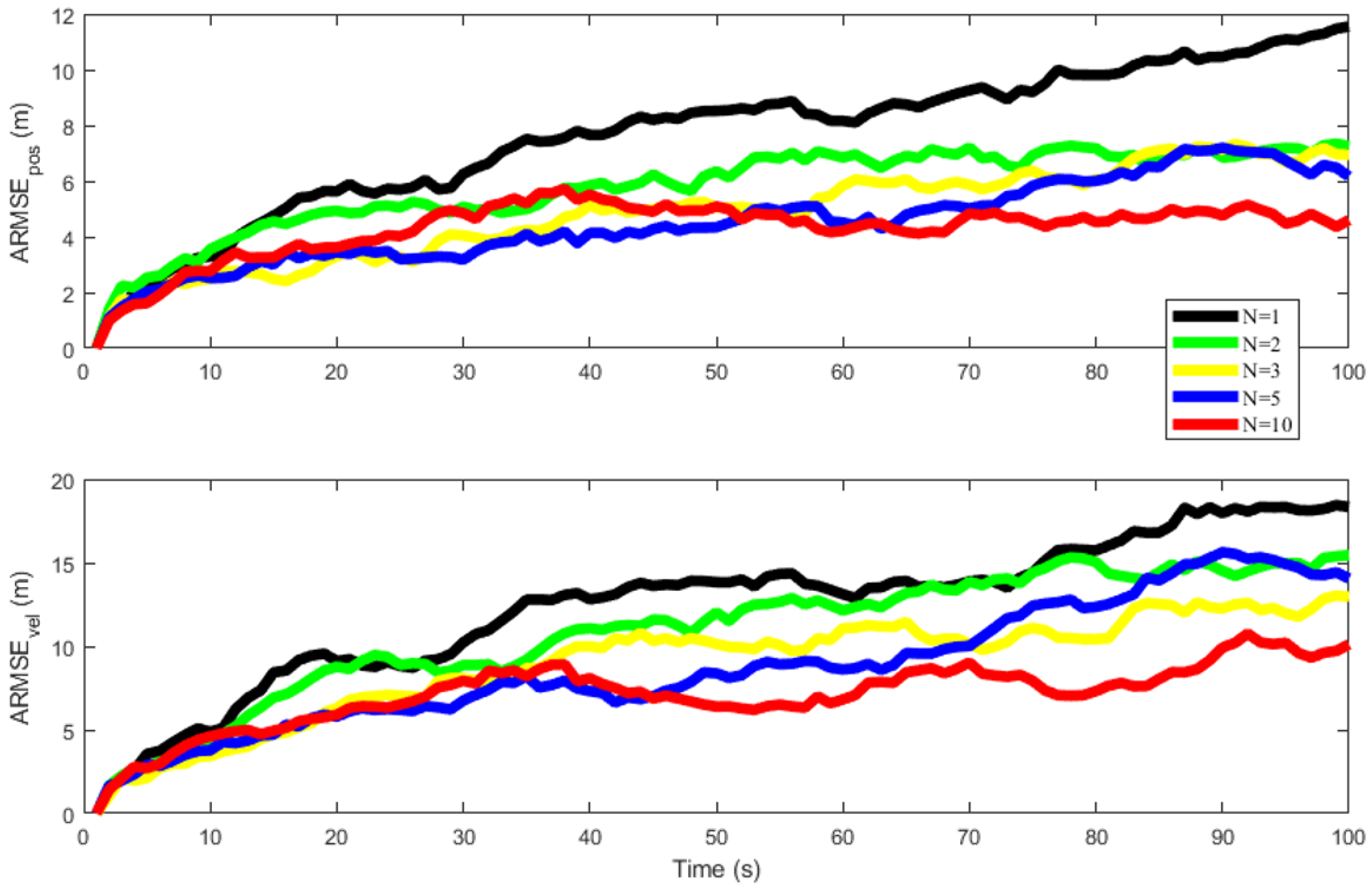
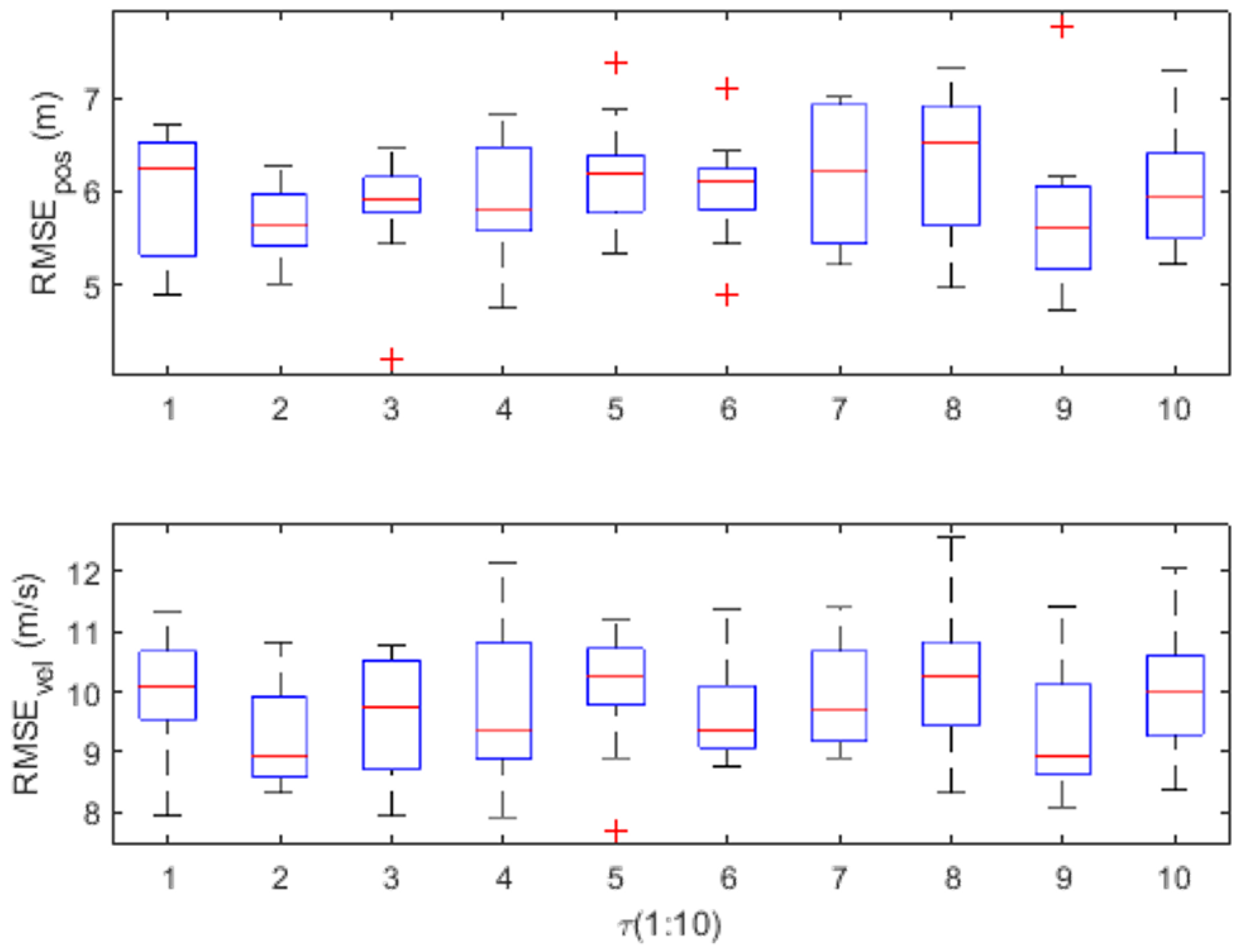
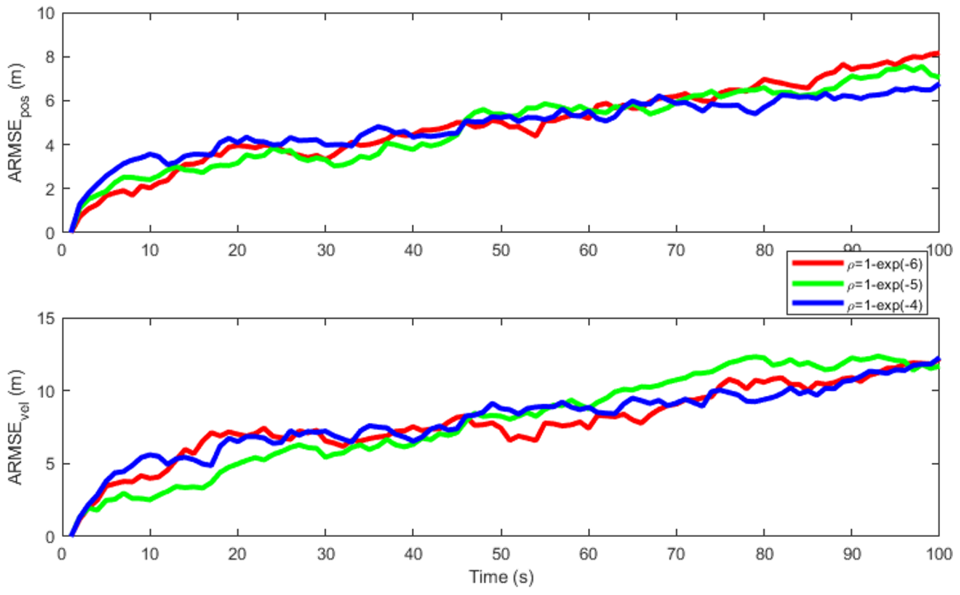
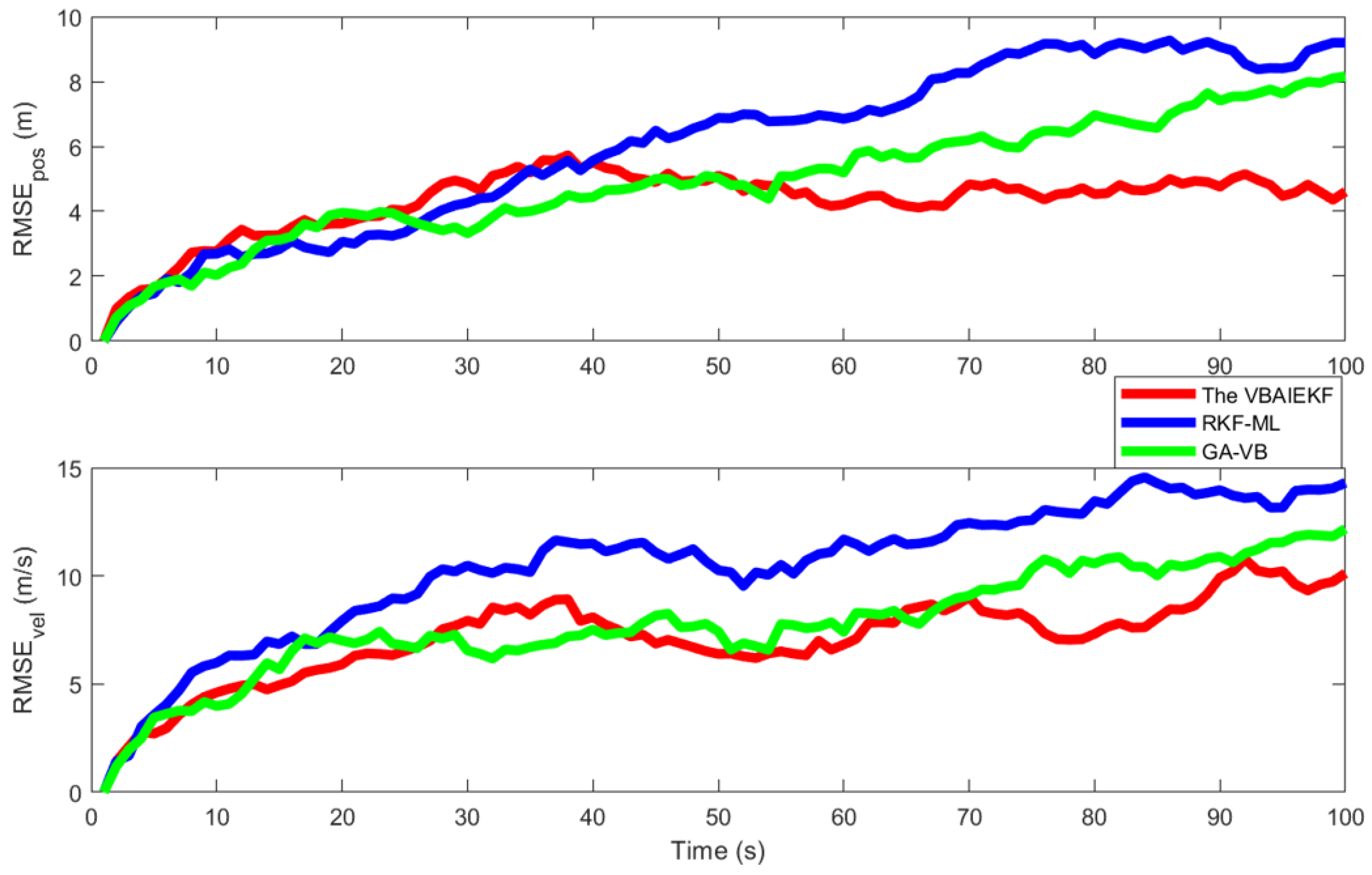
3.1. Two-Dimensional Target Tracking

In order to showcase the effectiveness of the suggested algorithm, we will employ the conventional scenario of two-dimensional target tracking and conduct a comparative analysis with various relevant approaches [38]. The state equation is represented as Equation (44). The observation quantity includes the target’s distance and bearing, and the observation equation is given as Equation (45):

$$x_t=\left[\begin{array}{cc}{\mathrm{I}}_2& {\mathrm{TI}}_2\\ 0_2& {\mathrm{I}}_2\end{array}\right]x_{t-1}+w_{t-1}$$

(44)

$$z_t=\left[\begin{array}{c}\sqrt{x_t^2+y_t^2}\\ arctan\frac{y_t}{x_t}\end{array}\right]x_t+v_t$$

(45)

where $x_t={\left[x_t,y_t,{\dot{x}}_t,{\dot{y}}_t\right]}^{\mathrm{T}}$ is the state of the target at moment $j,\left(x_t,y_t\right)$ is the position state, $\left({\dot{x}}_t,{\dot{y}}_t\right)$ is the velocity state in x and y directions. $T=1\mathrm{s}$ is the sampling time. $w_{t-1}$ is the zero-mean Gaussian process noise with the covariance $\overline{Q}=\left[\begin{array}{cc}\frac{T^3}{3}{\mathrm{I}}_2& \frac{T^2}{2}{\mathrm{I}}_2\\ \frac{T^2}{2}{\mathrm{I}}_2& T{\mathrm{I}}_2\end{array}\right]$.

The initial position and velocity of the state are as $x_0=\left[100\mathrm{m},100\mathrm{m},10{\mathrm{ms}}^{-1}\right.$, ${\left.10{\mathrm{ms}}^{-1}\right]}^{\mathrm{T}}$, with covariance $P_0=diag{\left(20{\mathrm{m}}^2,20{\mathrm{m}}^2,2{\mathrm{m}}^2{\mathrm{s}}^{-2},2{\mathrm{m}}^2{\mathrm{s}}^{-2}\right)}^{\mathrm{T}}$. The typical heavy-tailed noise is selected $\mathrm{d}$ as the measurement noise, and the Gaussian mixture distribution is used:

$$v_i\sim 0.8\mathcal{N}(0,\overline{R})+0.2\mathcal{N}(0,100\overline{R})$$

(46)

where $\overline{R}=diag\left({\left(5\mathrm{m}\right)}^2,{\left(0.05\mathrm{rad}\right)}^2\right)$ is the measurement noise covariance, and set $\epsilon ={10}^{-6}$. In the simulation experiment, the improved robust GA-VB [32], RKF-ML [33], and the proposed VBAIEKF were used to test the filtering effect. In the proposed VBAIEKF and the improved robust GA-VB and RKF-ML, the individual parameters were set as follows: parameter $b=5$, parameter $a=1$, parameter $u=4$, parameter $U=\tau \overline{R}$, forgetting factor $\rho =1-exp(-4)$, adjustment factor $\tau =6$, and the number of iterations $N=1,2,3,5,10$. All algorithms were coded with MATLAB R2020b on a computer.

To compare the state estimation accuracy of the aforementioned nonlinear filtering algorithms, the root mean square error (RMSE) [39] and the average root mean square error (ARMSE) of the state vector is chosen to represent the filtering accuracy, and is defined as follows:

$$RMS{E}_{\mathrm{pos}}=\sqrt{\frac{1}{N}{\displaystyle \sum _{n=1}^N}\left({\left(m_t^n-{\widehat{m}}_t^n\right)}^2+{\left(r_t^n-{\widehat{r}}_t^n\right)}^2\right)}$$

(47)

$$RMS{E}_{vel}=\sqrt{\frac{1}{N}{\displaystyle \sum _{n=1}^N}\left({\left({\dot{m}}_t^n-{\widehat{\dot{m}}}_t^n\right)}^2+{\left({\dot{r}}_t^n-{\widehat{\dot{r}}}_t^n\right)}^2\right)}$$

(48)

$$ARMS{E}_{pos}=\sqrt{\frac{1}{NT}{\displaystyle \sum _{t=1}^T}{\displaystyle \sum _{n=1}^N}\left({\left(m_t^n-{\widehat{m}}_t^n\right)}^2+{\left(r_t^n-{\widehat{r}}_t^n\right)}^2\right)}$$

(49)

$$ARMS{E}_{vel}=\sqrt{\frac{1}{NT}{\displaystyle \sum _{t=1}^T}{\displaystyle \sum _{n=1}^N}\left({\left({\dot{m}}_t^n-{\widehat{\dot{m}}}_t^n\right)}^2+{\left({\dot{r}}_t^n-{\widehat{\dot{r}}}_t^n\right)}^2\right)}$$

(50)

where $\left(m_t^n,r_t^n\right)$ is the true position, $\left({\widehat{m}}_t^n,{\widehat{r}}_t^n\right)$ is the estimated position, and N denotes the number of times the algorithm is run.

In Figure 1, the impact of iteration numbers on the VBAIEKF algorithm is examined. The iteration count influences the proposed VBAIEKF in a distinct manner, with values set at $N=1,2,3,5,10$. The observed trend indicates that as the number of iterations increases, the convergence speed gradually decreases, while the computational load correspondingly increases. Analysis of the ARMSE in position and velocity reveals a clear pattern; the ARMSE values demonstrate that accuracy improves with an increase in iterations, ultimately converging. When the iteration count reaches $N=10$, the ARMSE values tend to stabilize. This iterative improvement is significant, despite the anticipated increase in computational demands.

In Figure 2, a detailed examination is conducted to measure the impact of the adjustment factor $\tau$ on the performance of the proposed VBAIEKF algorithm. The adjustment factor $\tau$ systematically varies within the range of $\tau =1,2,3,5\dots ,10$. The results demonstrate that throughout the entire random process, the algorithm is uniformly influenced within a predetermined stable range. Notably, the operation of the algorithm is subject to a slight but not significant influence by the adjustment factor and minimization and precision enhancement. The VBAIEKF exhibits low sensitivity to parameters, displaying minimal influence from varying parameters. Therefore, $\tau =6$ was selected. This influence consistently remains within a specific stable range throughout the random process. At $\tau =6$, the algorithm achieves an optimal balance between error algorithm comparison experiments.

In Figure 3, we conducted a comprehensive analysis to evaluate the impact of the forgetting factor $\rho$ on the performance of the proposed VBAIEKF algorithm. Systematic variations of the variable $\rho$ within a certain range can identify various factors affecting the algorithm’s performance. Affecting the $\rho$ algorithm’s performance, $\rho =1-exp(-4)$, the impact of the forgetting factor significantly diminishes, thereby accelerating the convergence speed, reducing the RMSE, and making the algorithm output trajectory more perfect. The current configuration appears to have achieved the optimal balance between convergence speed, accuracy, and overall stability. Therefore, we chose $\rho =1-exp(-4)$ for the subsequent comparative analysis.

Table 1. $ARMS{E}_{pos}$, $ARMS{E}_{vel}$ and the average execution time for the RKF-ML, GA-VB, and VBAIEKF under different noise.

Algorithms and Noise		Values
Algorithms	Noise	${\mathit{ARMSE}}_{\mathit{p}\mathit{o}\mathit{s}}\left(\mathrm{m}\right)$	${\mathit{ARMSE}}_{\mathit{v}\mathit{e}\mathit{l}}(\mathrm{m}/\mathrm{s})$	$\mathit{Time}(\mathrm{s}$)
RKF-ML	$\overline{R}=diag\left({\left(1\mathrm{m}\right)}^2,{\left(0.01\mathrm{rad}\right)}^2\right)$	6.3241 (+4.25%)	7.5472 (−3.54%)	0.31657
	$\overline{R}=diag\left({\left(5\mathrm{m}\right)}^2,{\left(0.05\mathrm{rad}\right)}^2\right)$	6.0665 (0%)	7.8242 (0%)	0.32264
	$\overline{R}=diag\left({\left(10\mathrm{m}\right)}^2,{\left(0.1\mathrm{rad}\right)}^2\right)$	6.3854 (+5.26%)	7.6821 (−1.82%)	0.33187
GA-VB	$\overline{R}=diag\left({\left(1\mathrm{m}\right)}^2,{\left(0.01\mathrm{rad}\right)}^2\right)$	4.8532 (−1.65%)	10.3365 (−1.03%)	0.11242
	$\overline{R}=diag\left({\left(5\mathrm{m}\right)}^2,{\left(0.05\mathrm{rad}\right)}^2\right)$	4.9348 (0%)	10.4445 (0%)	0.11754
	$\overline{R}=diag\left({\left(10\mathrm{m}\right)}^2,{\left(0.1\mathrm{rad}\right)}^2\right)$	4.9938 (+1.196%)	10.5564 (+1.07%)	0.12432
The VBAIEKF	$\overline{R}=diag\left({\left(1\mathrm{m}\right)}^2,{\left(0.01\mathrm{rad}\right)}^2\right)$	4.3034 (+0.058%)	7.1024 (−0.17%)	0.10128
	$\overline{R}=diag\left({\left(5\mathrm{m}\right)}^2,{\left(0.05\mathrm{rad}\right)}^2\right)$	4.3009 (0%)	7.1147 (0%)	0.11215
	$\overline{R}=diag\left({\left(10\mathrm{m}\right)}^2,{\left(0.1\mathrm{rad}\right)}^2\right)$	4.3259 (+0.58%)	7.2658 (+0.21%)	0.11393

provides a comprehensive summary of the relative performance of the proposed VBAIEKF, GA-VB [32], and RKF-ML [33] at various levels of noise. Table 1 lists several key metrics: average root mean square error (ARMSE) for position and velocity, and average execution time. The results show that VBAIEKF has better convergence properties and adaptability. Compared to GA-VB and RKF-ML, the VBAIEKF shows a decrease in both the average position ARMSE and average velocity ARMSE, indicating improved accuracy in position and velocity estimation. Furthermore, this algorithm reduces the average execution time, highlighting its computational efficiency. Under various noise levels, using example noise $\overline{R}=diag\left({\left(5\mathrm{m}\right)}^2,{\left(0.05\mathrm{rad}\right)}^2\right)$ as a reference, the convergence ranges under noises $\overline{R}=diag\left({\left(1\mathrm{m}\right)}^2,{\left(0.01\mathrm{rad}\right)}^2\right)$ and $\overline{R}=diag\left({\left(10\mathrm{m}\right)}^2,{\left(0.1\mathrm{rad}\right)}^2\right)$ are computed. From Table 1, it is evident that the VBAIEKF algorithm under different levels of noise exhibits a position convergence range of +0.058%∼+0.58% and a velocity convergence range of −0.17%∼+0.21%, significantly smaller than RKF-ML and GA-VB. This indicates that the algorithm possesses excellent convergence and adaptability. Comparative analysis reveals that the proposed VBAIEKF is a highly reliable and effective solution, surpassing both GA-VB and RKF-ML methods across different noise levels. The results obtained in this study provide robust evidence of the reliability and effectiveness of the proposed VBAIEKF in various scenarios. The results of these studies confirm that this algorithm can be used as a reliable and efficient tool.

Figure 4 presents a thorough comparative analysis, wherein the proposed VBAIEKF algorithm is juxtaposed with existing optimization algorithms GA-VB and RKF-ML in terms of the noise $\overline{R}=diag\left({\left(5\mathrm{m}\right)}^2,{\left(0.05\mathrm{rad}\right)}^2\right)$, a specific number of iterations ($N=10$). The comparative analysis is based on the root mean square absolute error (ARMSE) of velocity and position estimates. The results underscore the efficacy of the VBAIEKF algorithm; compared to the existing optimization algorithms RKF-ML and GA-VB, the VBAIEKF exhibited significant improvements in $RMS{E}_{pos}$ and $RMS{E}_{vel}$, with increases of 21.81% and 22.11%, respectively. Table 1 shows that under noise $\overline{R}=diag\left({\left(5\mathrm{m}\right)}^2,{\left(0.05\mathrm{rad}\right)}^2\right)$, the convergence speed was enhanced by 49.04%, demonstrating accelerated convergence and significantly enhanced estimation precision. This highlights the algorithm’s capacity to provide reliable and accurate estimates.

3.2. Nonlinear Numerical UNGM

This paper employs a nonlinear numerical UNGM [40] to demonstrate the effectiveness of VBRAIEKF. The equation representing the state space of the UNGM model is as follows:

$$\left\{\begin{array}{c}{x}_k=0.5x_{k-1}+25\frac{x_{k-1}}{1+x_{k-1}^2}+8cos\left(1.2(k-1)\right)+v_{k-1}\hfill \\ y_k=x_k^2/20+r_k\hfill \end{array}\right.$$

(51)

where $Q_{k-1}$ and ${\mathrm{r}}_{\mathrm{k}}$ represent measurement noise with a mean of zero and covariance, and $v_{k-1}$ represents non-Gaussian process noise $R_k$.

The measurement noise is selected to be the typical heavy-tailed noise [25].

$$v_i\sim 0.9\mathcal{N}(0,\overline{R})+0.1\mathcal{N}(0,100\overline{R})$$

(52)

The symbol $\overline{R}$ represents the measurement noise covariance matrix, which is defined as $diag\left({\left(1\mathrm{m}\right)}^2,{\left(0.01\mathrm{rad}\right)}^2\right)$. By adjusting the parameters to optimize the algorithm’s performance, setting the forgetting factor $\rho =1-exp(-4)$ significantly reduces its impact, resulting in a significant decrease in influence. By selecting $\epsilon ={10}^{-6}$, the algorithm’s convergence speed is greatly enhanced. By setting the tuning factor $\tau =6$, the algorithm attains an optimal equilibrium in error algorithm comparative experiments. Performing 10 iterations decreases the average root mean square error (ARMSE), resulting in a more precise trajectory for the algorithm’s output. During the simulation experiment, GA-VB, RKF-ML, and VBAIEKF are employed to evaluate the filtering efficacy.

Figure 5 examines the comparability of $RMS{E}_{pos}$ and $RMS{E}_{vel}$ for the GA-VB, RKF-ML, and the VBAIEKF algorithms. The results indicate that the estimation state of VBAIEKF demonstrates higher precision, with RMSE values lower than those of GA-VB and RKF-ML. It can more accurately estimate the expected state covariance and the actual state covariance. The improvement in estimation accuracy for both position and velocity signifies its reliability.

4. Conclusions

We have successfully developed an improved adaptive iterative extended Kalman filter based on variational Bayesian for nonlinear situations (VBAIEKF). This innovative approach not only enhances the accuracy of state estimation and broadens the applicability of the algorithm in dynamic and complex environments but also addresses the issue of algorithm parameter sensitivity. The foundation of this algorithm is the principle of variational Bayesian, which significantly boosts its capability to handle uncertainties and effectively resolve nonlinear problems. Through extensive simulation experiments, the convergence of the algorithm under various conditions, including different noise levels and outlier scenarios, has been confirmed. Our research results emphasize the algorithm’s resilience, demonstrating its ability to maintain stability and accurate estimation in challenging and unpredictable situations. Compared with existing algorithms, the VBAIEKF shows advantages in multiple aspects:

(1) The VBAIEKF achieves enhanced estimation accuracy, with a 21.81% improvement in position estimation precision and a 22.11% improvement in velocity estimation.

(2) The VBAIEKF exhibits superior convergence characteristics and adaptability to different noise levels, with a position convergence range of +0.058%∼+0.58% and a velocity convergence range of −0.17%∼+0.21%.

(3) The VBAIEKF demonstrates low sensitivity to various parameters, addressing the impact of parameters on the outcomes.

(4) The VBAIEKF attains heightened operational efficiency with lower complexity, resulting in a 49.04% increase in convergence speed.

In future research endeavours, validation of robustness and stability will be pursued. This exploration will unfold on two fronts: one involving theoretical substantiation and the other focusing on the real variability of the experimental process of the experimental process and the treatment of noise anomalies.

References

1. Shen, Q.; Jiang, B.; Shi, P.; Zhao, J. Cooperative Adaptive Fuzzy Tracking Control for Networked Unknown Nonlinear Multiagent Systems with Time-Varying Actuator Faults. IEEE Trans. Fuzzy Syst. 2014, 22, 494–504. [Google Scholar] [CrossRef]
2. Wang, J.; Liu, Z.; Chen, H.; Zhang, Y.; Zhang, D.; Peng, C. Trajectory Tracking Control of a Skid-Steer Mobile Robot Based on Nonlinear Model Predictive Control with a Hydraulic Motor Velocity Mapping. Appl. Sci. 2024, 14, 122. [Google Scholar] [CrossRef]
3. Petrov, E.P.; Kharina, N.L. Digital Radar Imaging by Nonlinear Filtering Methods of Discrete and Continuous Parameters (Amplitude and Delay) of Reflected PM Signals. In Proceedings of the 2020 Dynamics of Systems, Mechanisms and Machines (Dynamics), Omsk, Russia, 10–12 November 2020; pp. 1–6. [Google Scholar] [CrossRef]
4. Senel, N.; Kefferpütz, K.; Doycheva, K.; Elger, G. Multi-Sensor Data Fusion for Real-Time Multi-Object Tracking. Processes 2023, 11, 501. [Google Scholar] [CrossRef]
5. Rahimi, F.; Rezaei, H. A Distributed Fault Estimation Approach for a Class of Continuous-Time Nonlinear Networked Systems Subject to Communication Delays. IEEE Control. Syst. Lett. 2022, 6, 295–300. [Google Scholar] [CrossRef]
6. Li, Z.; Zhong, L.; Yang, H.; Zhou, L. Distributed Cooperative Tracking Control Strategy for Virtual Coupling Trains: An Event-Triggered Model Predictive Control Approach. Processes 2023, 11, 3293. [Google Scholar] [CrossRef]
7. Li, B.; Xiao, M. Nonlinear algorithm based on new Kalmanfiltering method for integrated SINS/GPS Navigation System. In Proceedings of the 2009 IEEE International Conference on Intelligent Computing and Intelligent Systems, Shanghai, China, 20–22 November 2009; pp. 557–561. [Google Scholar] [CrossRef]
8. Sun, X.; Cai, M.; Ding, J. A GPU-Accelerated Method for 3D Nonlinear Kelvin Ship Wake Patterns Simulation. Appl. Sci. 2023, 13, 12148. [Google Scholar] [CrossRef]
9. Eremin, E.L.; Nikiforova, L.V.; Shelenok, E.A. Combined Nonlinear Control System for Non-Affine Multi-Loop Plant with Control and State Delays. In Proceedings of the 2022 4th International Conference on Control Systems, Mathematical Modeling, Automation and Energy Efficiency (SUMMA), Lipetsk, Russia, 9–11 November 2022; pp. 23–29. [Google Scholar] [CrossRef]
10. Sha’aban, Y.A. Distributed Control of an Ill-Conditioned Non-Linear Process Using Control Relevant Excitation Signals. Processes 2023, 11, 3320. [Google Scholar] [CrossRef]
11. Kai, G.; Zhang, W. Numerical study of a class of nonlinear financial system. J. Dyn. Control 2016, 14, 407–411. [Google Scholar]
12. Zhang, Y.; Wang, Z. Statistics Character and Complexity in Nonlinear Systems. In Machine Learning; InTechOpen: London, UK, 2010. [Google Scholar]
13. Zhang, Y.; Wu, W.; He, W.; Zhao, N. Algorithm Design and Convergence Analysis for Coexistence of Cognitive Radio Networks in Unlicensed Spectrum. Sensors 2023, 23, 9705. [Google Scholar] [CrossRef]
14. Huang, Y.; Zhang, Y.; Li, N.; Chambers, J. A Robust Gaussian Approximate Fixed-Interval Smoother for Nonlinear Systems with Heavy-Tailed Process and Measurement Noises. IEEE Signal Process. Lett. 2016, 23, 468–472. [Google Scholar] [CrossRef]
15. Xu, D.; Wang, B.; Zhang, L.; Chen, Z. A New Adaptive High-Degree Unscented Kalman Filter with Unknown Process Noise. Electronics 2022, 11, 1863. [Google Scholar] [CrossRef]
16. Zhao, J. Dynamic State Estimation with Model Uncertainties Using H Extended Kalman Filter. IEEE Trans. Power Syst. 2018, 33, 1099–1100. [Google Scholar] [CrossRef]
17. Luo, X.; Zhao, J.; Xiong, Y.; Xu, H.; Chen, H.; Zhang, S. Parameter Identification of Five-Phase Squirrel Cage Induction Motor Based on Extended Kalman Filter. Processes 2022, 10, 1440. [Google Scholar] [CrossRef]
18. Huang, W.; Fu, H.; Zhang, W. A Novel Robust Variational Bayesian Filter for Unknown Time-Varying Input and Inaccurate Noise Statistics. IEEE Sensors Lett. 2023, 7, 7001104. [Google Scholar] [CrossRef]
19. Lu, X.; Jing, D.; Jiang, D.; Gao, Y.; Yang, J.; Li, Y.; Li, W.; Tao, J.; Liu, M. Trajectory PHD Filter for Adaptive Measurement Noise Covariance Based on Variational Bayesian Approximation. Appl. Sci. 2022, 12, 6388. [Google Scholar] [CrossRef]
20. Huang, Y.; Zhang, Y.; Xu, B.; Wu, Z.; Chambers, J.A. A New Adaptive Extended Kalman Filter for Cooperative Localization. IEEE Trans. Aerosp. Electron. Syst. 2018, 54, 353–368. [Google Scholar] [CrossRef]
21. Liu, Z.; Chen, S.; Wu, H.; Chen, K. Robust Student’s t Mixture Probability Hypothesis Density Filter for Multi-Target Tracking with Heavy-Tailed Noises. IEEE Access 2018, 6, 39208–39219. [Google Scholar] [CrossRef]
22. Huang, H.; Zhang, H. Student’s t-Kernel-Based Maximum Correntropy Kalman Filter. Sensors 2022, 22, 1683. [Google Scholar] [CrossRef] [PubMed]
23. Chang, L.; Li, K.; Hu, B. Huber’s M-Estimation-Based Process Uncertainty Robust Filter for Integrated INS/GPS. IEEE Sensors J. 2015, 15, 3367–3374. [Google Scholar] [CrossRef]
24. Gao, W.; Liu, Y.; Xu, B. Robust Huber-Based Iterated Divided Difference Filtering with Application to Cooperative Localization of Autonomous Underwater Vehicles. Sensors 2014, 14, 24523–24542. [Google Scholar] [CrossRef] [PubMed]
25. Wang, G.; Zhang, Y.; Wang, X. Iterated maximum correntropy unscented Kalman filters for non-Gaussian systems. Signal Process. 2019, 163, 87–94. [Google Scholar] [CrossRef]
26. Wang, J.; Zhang, H.; Hao, P.; Deng, H. Observer-Based Approximate Affine Nonlinear Model Predictive Controller for Hydraulic Robotic Excavators with Constraints. Processes 2023, 11, 1918. [Google Scholar] [CrossRef]
27. Zhang, H.; Yang, Z.; Xiong, H.; Zhu, T.; Long, Z.; Wu, W. Transformer Aided Adaptive Extended Kalman Filter for Autonomous Vehicle Mass Estimation. Processes 2023, 11, 887. [Google Scholar] [CrossRef]
28. Wang, H.; Li, H.; Zhang, W.; Zuo, J.; Wang, H. Derivative-Free Huber-Kalman Smoothing Based on Alternating Minimization. Signal Process. 2019, 163, 115–122. [Google Scholar] [CrossRef]
29. Wang, X.; Cui, N.; Guo, J. Huber-based Unscented Filtering and its Application to Vision-based Relative Navigation. Radar Sonar Navig. Iet 2010, 4, 134–141. [Google Scholar] [CrossRef]
30. Wei, X.; Hua, B.; Wu, Y.; Chen, Z. Robust Interacting Multiple Model Cubature Kalman Filter for Nonlinear Filtering with Unknown Non-Gaussian Noise. Digit. Signal Process. 2023, 136, 103982. [Google Scholar] [CrossRef]
31. Kheirish, M.; Yazdi, E.A.; Mohammadi, H.; Mohammadi, M. A Fault-tolerant Sensor Fusion in Mobile Robots Using Multiple Model Kalman Filters. Robot. Auton. Syst. 2023, 161, 104343. [Google Scholar] [CrossRef]
32. Huang, Y.; Zhang, Y.; Li, N.; Chambers, J. A Robust Gaussian Approximate Filter for Nonlinear Systems with Heavy Tailed Measurement Noises. In Proceedings of the 2016 IEEE International Conference on Acoustics, Speech and Signal Processing (ICASSP), Shanghai, China, 20–25 March 2016; pp. 4209–4213. [Google Scholar] [CrossRef]
33. Wang, G.; Yang, C.; Ma, X. A Novel Robust Nonlinear Kalman Filter Based on Multivariate Laplace Distribution. IEEE Trans. Circuits Syst. II Express Briefs 2021, 68, 2705–2709. [Google Scholar] [CrossRef]
34. Jacquemin, T.; Tomar, S.; Agathos, K.; Mohseni-Mofidi, S.; Bordas, S.P.A. Taylor-series Expansion based Numerical Methods: A Primer, Performance Benchmarking and New Approaches for Problems with Mon-smooth Solutions. Arch. Comput. Methods Eng. 2020, 27, 1465–1513. [Google Scholar] [CrossRef]
35. Blei, D.M.; Kucukelbir, A.; Mcauliffe, J.D. Variational Inference: A Review for Statisticians. J. Amer. Statist. Assoc. 2017, 112, 859–877. [Google Scholar] [CrossRef]
36. Dong, P.; Jing, Z.; Leung, H.; Shen, K. Variational Bayesian adaptive cubature information filter based on Wishart distribution. IEEE Trans. Autom. Control 2017, 2, 6051–6057. [Google Scholar] [CrossRef]
37. Huang, Y.; Zhang, Y.; Shi, P.; Chambers, J. Variational Adaptive Kalman Filter with Gaussian-Inverse-Wishart Mixture Distribution. IEEE Trans. Autom. Control 2021, 66, 1786–1793. [Google Scholar] [CrossRef]
38. Wang, G.; Zhang, Y.; Wang, X. Maximum Correntropy Rauch-Tung-Striebel Smoother for Nonlinear and Non-Gaussian Systems. IEEE Trans. Autom. Control 2021, 66, 1270–1277. [Google Scholar] [CrossRef]
39. Chai, T.; Draxler, R.R. Root Mean Square Error (RMSE) or Mean Absolute Error (MAE)?—Arguments Against Avoiding RMSE in the Literature. Geosci. Model Dev. 2014, 7, 1247–1250. [Google Scholar] [CrossRef]
40. Liu, X.; Liu, X.; Yang, Y.; Gao, Y.; Zhang, W. Variational Bayesian-Based Robust Cubature Kalman Filter with Application on SINS/GPS Integrated Navigation System. IEEE Sensors J. 2022, 22, 489–500. [Google Scholar] [CrossRef]
Figure 1. A R M S E p o s  and  A R M S E v e l  for different iterations N.
Applsci 14 01393 g001
Figure 2. R M S E p o s  and  R M S E v e l  for different adjustment factor  τ .
Applsci 14 01393 g002
Figure 3. A R M S E p o s  and  A R M S E v e l  for different forgetting factor  ρ .
Applsci 14 01393 g003
Figure 4. R M S E p o s  and  R M S E v e l  for different algorithms.
Applsci 14 01393 g004
Figure 5. R M S E p o s  and  R M S E v e l  for different algorithms.
Applsci 14 01393 g005