Multi-Head Transformer Architecture with Higher Dimensional Feature Representation for Massive MIMO CSI Feedback

Abstract

To achieve the anticipated performance of massive multiple input multiple output (MIMO) systems in wireless communication, it is imperative that the user equipment (UE) accurately feeds the channel state information (CSI) back to the base station (BS) along the uplink. To reduce the feedback overhead, an increasing number of deep learning (DL)-based networks have emerged, aimed at compressing and subsequently recovering CSI. Various novel structures are introduced, among which Transformer architecture has enabled a new level of precision in CSI feedback. In this paper, we propose a new method named TransNet+ built upon the Transformer-based TransNet by updating the multi-head attention layer and implementing an improved training scheme. The simulation results demonstrate that TransNet+ outperforms existing methods in terms of recovery accuracy and achieves state-of-the-art.

1. Introduction

Massive multiple input multiple output (MIMO) makes a substantial contribution to augmenting the throughput of wireless communication systems and providing high-speed data services, which is essential in future mobile communication systems [1,2]. Massive MIMO systems can be categorized into two principal domains: time division duplexing (TDD) systems and frequency division duplexing (FDD) systems where orthogonal time and frequency are recognized to distinguish the uplink and downlink [3,4]. A critical prerequisite for achieving the desired transmission quality in massive MIMO is the availability of perfect channel state information (CSI) at both the base station (BS) and the user equipment (UE). Leveraging the accurate CSI, the BS can design the appropriate precoding vector, thus improving the transmission quality. This is especially significant in FDD systems because, unlike in TDD systems where channel reciprocity is taken into account, the CSI of the downlink cannot be directly obtained from the channel estimation at the BS [5,6,7]. The CSI at the BS in FDD systems relies heavily on accurate feedback from the UE in real time, which poses a formidable challenge since the feedback overhead increases in a linear manner as the number of antennas grows [8].

To reduce the feedback cost, scholars naturally explore techniques for compressing the downlink CSI at the UE and subsequently recovering the original CSI at the BS. A variety of schemes have been devised to narrow the gap between the recovered CSI and the actual CSI. Conventional methods for CSI feedback, such as those utilizing codebooks and compressive sensing (CS), struggle to balance low complexity with high accuracy. Therefore, CSI compression and feedback mechanisms in massive MIMO systems have begun leveraging deep learning (DL) technologies. This approach is inspired by the autoencoder architecture commonly used in image compression. The deep learning based methods can be divided into two categories, one focusing on improving the performance of CSI feedback with novel neural network (NN) architecture design and multi-domain correlation utilization, the other favoring joint design with other modules and practical consideration to promote the practical deployment of DL-based CSI feedback.

In recent years, the Transformer architecture designed for natural language processing (NLP), which is marked by the attention mechanism, has been applied to numerous research areas [9]. A convolutional Transformer structure named CsiFormer is proposed in [10] to compensate for NN methods’ deficiency in long-range dependency. TransNet [11] presents a two-layer Transformer architecture, enabling the encoder to learn connections between various parts of the CSI during feedback. Its outstanding results underscore the immense potential of the Transformer architecture in the realm of CSI feedback. According to TransNet, higher dimensional feature representation is beneficial to obtain higher-resolution CSI features. In this paper, we first use feature representation with higher dimensions to improve the feedback quality of the model at high compression rates. Secondly, the warm-up-aided cosine training scheme proposed in [12] is exploited. It can not only accelerate the training speed, but also enhance the model’s capacity to learn high-resolution features. We present a comprehensive analysis that includes FLOPs and recovery accuracy for different models based on the attention mechanism in CSI feedback. Furthermore, we conduct a comparative experiment to investigate the impact of varying numbers of attention heads within the multi-head attention layer. The major contributions of our work can be summarized as follows:

• Based on the standard Transformer architecture, we propose a two-layer Transformer network for CSI feedback, which is capable of better characterizing the CSI and thus improving the recovery accuracy;
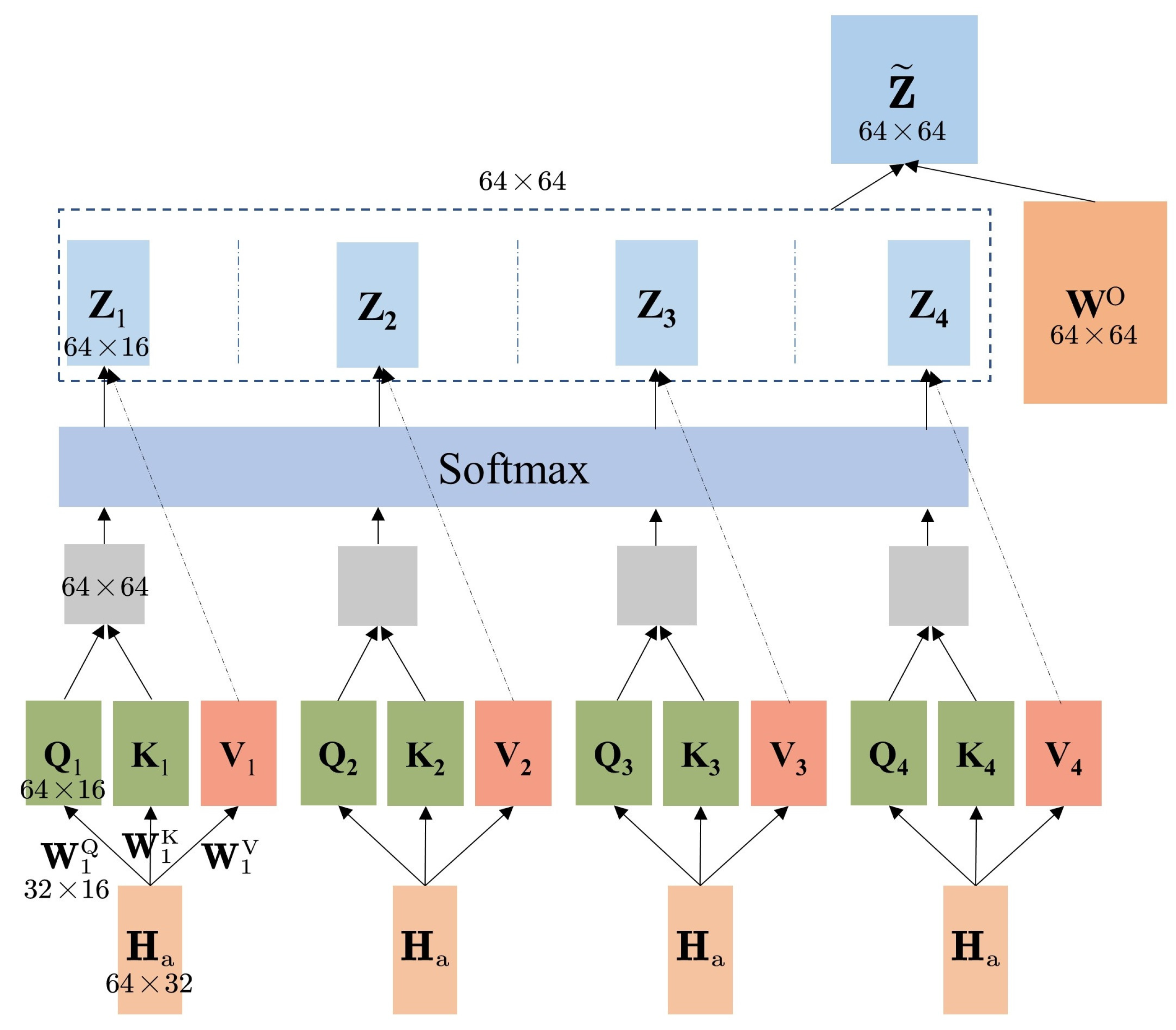
• We adopt higher dimensional feature representation to improve the quality of feedback and increase the number of attention heads to jointly attend to information from different representation subspaces at different positions;
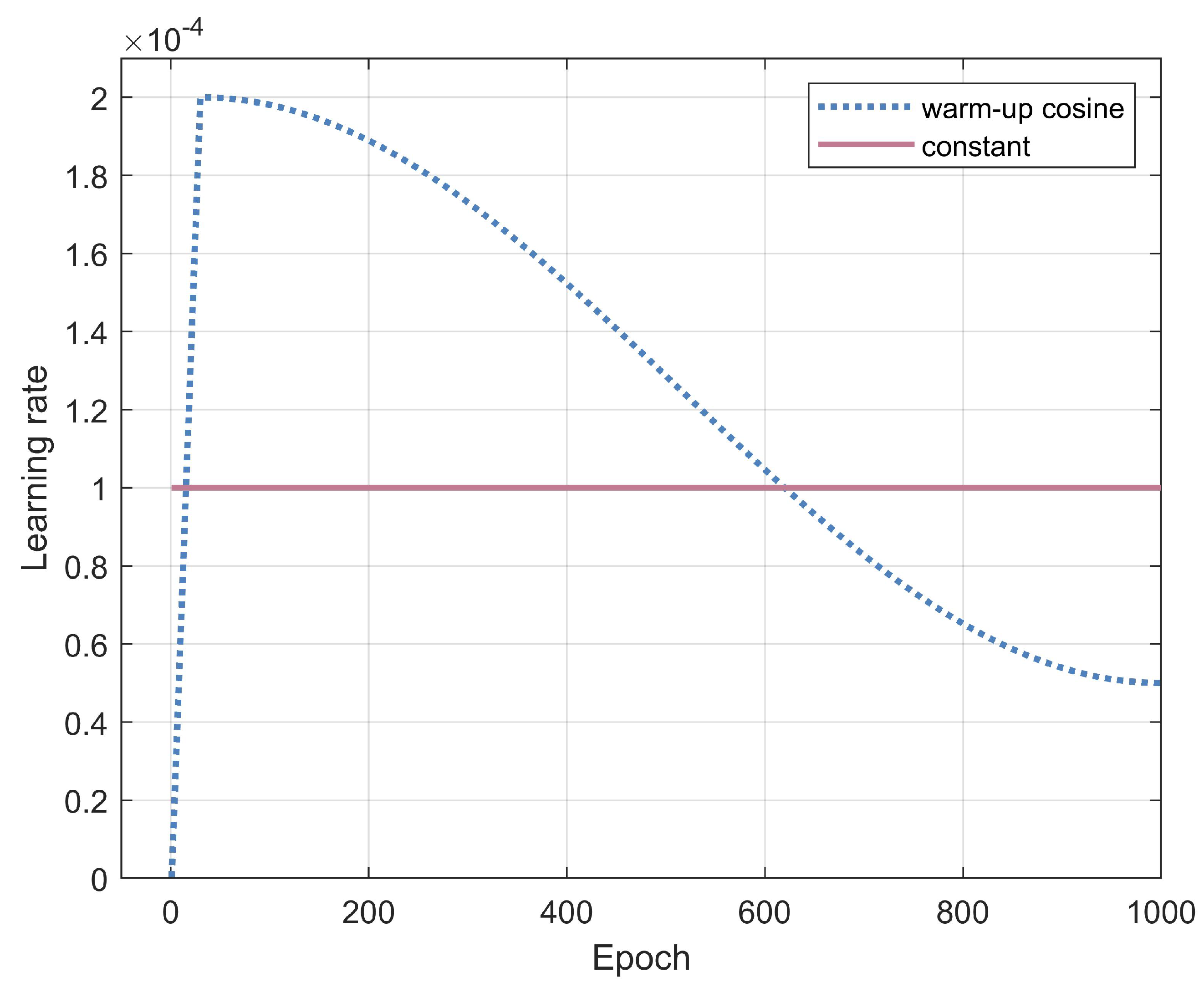
• The warm-up cosine training scheme is introduced for quicker convergence and stronger capability to learn high-resolution CSI features.

2. Related Work

More and more schemes are being designed to improve the effectiveness of CSI feedback and thus the signal transmission quality of massive MIMO systems. Firstly, CS methods commonly used in signal processing is introduced. However, the prerequisite for utilizing CS is that the channel is strongly sparse, which cannot be fully satisfied in practice [13]. In addition, CS methods do not fully exploit channel characteristics as random projection is performed and iterative CS methods may lead to slow reconstruction [14].

Machine learning, as an indispensable tool, has ushered in a revolution across various research domains, and it is no exception in CSI feedback [15]. Its branches, such as DL, reinforcement learning, and federated learning, are applied to different tasks [16]. As for CSI feedback, DL has gained widespread adoption. A convolutional neural network (CNN) named CsiNet is proposed in [14], demonstrating superior performance over traditional CS methods. Subsequent studies [12,17,18,19], such as CRNet [12] and CLNet [18], have been conducted to improve feedback performance with computational overhead reduced. CsiNet+ [20] incorporates refinement theory in DL, thereby improving the original CsiNet at the expense of higher floating point operations (FLOPs). Numerous works focus on introducing new structures to exploit channel properties. For instance, CsiNet-LSTM [21] and Attention-CsiNet [22] utilize the long short-time memory (LSTM) module and the attention mechanism, respectively. These two modules are synergistically combined in [8] to capture the temporal correlation of channels. Algorithm SALDR [23] leverages self-attention learning in conjunction with a dense RefineNet. Despite optimized performance, these approaches result in a substantial increase in FLOPs.

Multi-domain correlations have been adopted to leverage the geometrical wireless propagation information embedded within the CSI. For instance, the prediction neural network in [24] generates the current CSI based on the previous CSI sequence capitalizing on time correlation, which is shared by both the UE and the BS. Furthermore, the DualNet-MAG architecture in [25] exploits the correlation between the magnitudes of the bidirectional channels, with the uplink channel serving as a feedback channel for the quantized CSI phase and a neural network-based encoder compressing the CSI magnitude. The framework SampleDL [26] extracts the correlation between channels over adjacent subcarriers to further reduce the feedback cost. In addition, some recent works [27] make the most of the correlation between neighboring UEs.

Some methods concentrate on reducing the computational cost and optimizing the occupation of uplink bandwidth resources. MarkovNet [28] develops a deep CNN architecture based on the Markov chain with spherical normalization of the CSI, effectively lowering the computational complexity compared to other over-parameterized approaches. CAnet, which conducts downlink channel acquisition with the help of the uplink data, is designed in [29]. The approach encompasses pilot design, channel estimation, and feedback within a unified framework and saves notable feedback bits. In pursuit of reduced overhead and enhanced deployment compatibility, the authors of [30] propose an implicit feedback scheme named ImCsiNet. The UE spreads and superimposes the downlink CSI over the uplink UE data sequence in [31], which introduces DL to superimposed coding-based CSI feedback. Additionally, the BS extracts the downlink CSI and UE data from the received signal [32].

The remaining works focus on empowering the practical deployment of DL-based CSI feedback models. Given that the complete channel acquisition involves other modules such as channel estimation, joint training of multiple modules can not only simulate real communication scenarios but also maximize performance gains. Two joint channel estimation and feedback architecture named PFnet and CEFnet are introduced in [33]. Moreover, ref. [34] incorporates the pilot design and the precoding design in the training module. In consideration of various interferences and the non-linear influence along the feedback link, a plug-and-play denoising network based on residual learning is proposed in [35], which significantly enhances robustness during practical employment.

3. System Model

In this work, a single-cell massive MIMO FDD system equipped with $N_{\mathrm{t}}\gg 1$ antennas at BS and $N_{\mathrm{r}}$ antennas at UE is considered. For simplicity, $N_{\mathrm{r}}$ is set to 1. During downlink transmission, we apply orthogonal frequency division multiplexing (OFDM) and denote the number of subcarriers as $N_{\mathrm{c}}$. The received signal on the n-th subcarrier is given by

$$y_n={\tilde{\mathbf{h}}}_n^{\mathrm{H}}{\mathbf{p}}_n{x}_n+z_n$$

(1)

where ${\tilde{\mathbf{h}}}_n\in {\mathbb{C}}^{N_{\mathrm{t}}\times 1}$ is the channel vector in frequency domain, ${\mathbf{p}}_n\in {\mathbb{C}}^{N_{\mathrm{t}}\times 1}$ represents the precoding vector, $x_n$ represents the transmitted data symbol, and $z_n$ denotes the additive white Gaussian noise. We denote the channel matrix as $\tilde{\mathbf{H}}={\left[{\tilde{\mathbf{h}}}_0,{\tilde{\mathbf{h}}}_2,...,{\tilde{\mathbf{h}}}_{N_{\mathrm{c}}-1}\right]}^{\mathrm{H}}\in {\mathbb{C}}^{N_{\mathrm{c}}\times N_{\mathrm{t}}}$. We assume perfect channel estimation. At the receiver side, UE estimates the channel matrix and feeds this information back to BS. Based on the accurate CSI, BS can design the corresponding precoding vector, which will help improve the transmission quality.

According to the CSI matrix, the number of elements needed to be fed back is $2N_{\mathrm{c}}{N}_{\mathrm{t}}$ with the real and imaginary parts separated. Due to the large feedback overhead in massive MIMO systems, we need to design feedback schemes intentionally. First of all, we can take advantage of the CSI sparsity in the angular-delay domain resulting from short delay spread due to multipath effects [14]. $\tilde{\mathbf{H}}$ can be converted to $\mathbf{H}\in {\mathbb{C}}^{N_{\mathrm{c}}\times N_{\mathrm{t}}}$ in angular-delay domain by performing 2D discrete Fourier transform. The element of $\mathbf{H}$ at the k-th row and l-th column can be calculated by

$$h_{k,l}=\frac{1}{N_{\mathrm{c}}\times N_{\mathrm{t}}}\sum _{m=0}^{N_{\mathrm{c}}-1}\sum _{n=0}^{N_{\mathrm{t}}-1}{\tilde{h}}_{m,n}{e}^{-j2\pi \left(\frac{k}{N_{\mathrm{c}}}m+\frac{l}{N_{\mathrm{t}}}n\right)}$$

(2)

where $k=0,1,2,\dots ,N_{\mathrm{c}}-1$, $l=0,1,2,\dots ,N_{\mathrm{t}}-1$. After the processing, we find that most of the elements of $\mathbf{H}$ are close to zero except for the first $N_{\mathrm{a}}$ rows [17]. So, $\mathbf{H}$ can be replaced by a matrix ${\mathbf{H}}_{\mathrm{a}}$ consisting of the first $N_{\mathrm{a}}$ rows of itself without losing much information. Consequently, the number of parameters is reduced to $2N_{\mathrm{a}}{N}_{\mathrm{t}}$.

To further reduce the feedback overhead, we are supposed to do compression on ${\mathbf{H}}_{\mathrm{a}}$ before feedback and recover it after feedback. The whole feedback scheme can be derived as

$${\widehat{\mathbf{H}}}_{\mathrm{a}}=f_{\mathrm{re}}\left(f_{\mathrm{com}}\left({\mathbf{H}}_{\mathrm{a}},{\Theta }_{\mathrm{c}}\right),{\Theta }_{\mathrm{r}}\right)$$

(3)

where $f_{\mathrm{com}}\left(·\right)$ and $f_{\mathrm{re}}\left(·\right)$ denote the compression and recovery process, and ${\Theta }_{\mathrm{c}}$ and ${\Theta }_{\mathrm{r}}$ represent the parameters involved in the compression and recovery scheme. In our work, we assume a perfect feedback link where the compressed CSI can be transmitted to the BS without loss.

The aim of optimization is to obtain ${\Theta }_{\mathrm{c}}$ and ${\Theta }_{\mathrm{r}}$ by training to minimize the distance between ${\mathbf{H}}_{\mathrm{a}}$ and ${\widehat{\mathbf{H}}}_{\mathrm{a}}$, which can be concluded by

$$\left({\widehat{\Theta }}_{\mathrm{c}},{\widehat{\Theta }}_{\mathrm{r}}\right)=\underset{{\Theta }_{\mathrm{c}},{\Theta }_{\mathrm{r}}}{\arg min}{∥{\mathbf{H}}_{\mathrm{a}}-f_{\mathrm{re}}\left(f_{\mathrm{com}}\left({\mathbf{H}}_{\mathrm{a}},{\Theta }_{\mathrm{c}}\right),{\Theta }_{\mathrm{r}}\right)∥}_2^2$$

(4)

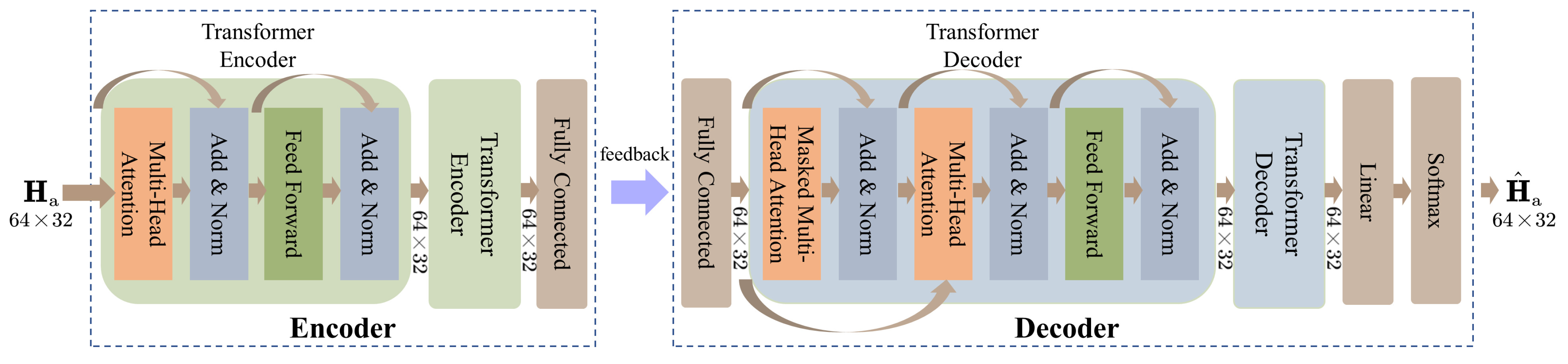
4. Structure of the Network and Training Scheme

4.1. Structure of the Network

The network consists of two identical encoder and decoder layers within the encoder and decoder modules, respectively. As illustrated in Figure 1, the CSI matrix is initially fed into the multi-head attention layer of the encoder. Subsequently, the input and output of the multi-head attention layer are sent into the add and norm layer, which combines them by skip connections. Next, the output of the add and norm layer enters the feed-forward layer. Similarly, another add and norm layer combines the input and output of the feed-forward layer. After transmitting the output of the second encoder layer into the fully connected layer, which compresses the matrix at a fixed compression rate, we obtain the output of the entire encoder. Compared to a Transformer encoder, a Transformer decoder starts with an additional masked multi-head attention layer and an add and norm layer. Notably, the multi-head attention layer of the decoder receives two inputs, the output of the first add and norm layer and the output of the fully connected layer of the decoder. Finally, processed by two decoder layers, the output is sent into the linear layer and the softmax layer. The network’s improvement in feedback accuracy is primarily attributed to the multi-head attention mechanism and the optimized training strategy.

4.2. Multi-Head Attention Layer

In Transformer architecture, the multi-head attention layer in Figure 1 is the core layer. Figure 2 shows the internal data processing of the layer. The particular attention function of Transformer is called Scaled Dot-Product Attention [36]. For each CSI matrix ${\mathbf{H}}_{\mathrm{a}}$, it is multiplied by ${\mathbf{W}}^{\mathrm{Q}}$, ${\mathbf{W}}^{\mathrm{K}}$, ${\mathbf{W}}^{\mathrm{V}}\in {\mathbb{R}}^{N_{\mathrm{t}}\times d_{\mathrm{model}}}$ to compute the corresponding query, key, and value matrix, which are denoted as $\mathbf{Q}$, $\mathbf{K}$, $\mathbf{V}$. ${\mathbf{W}}^{\mathrm{Q}}$, ${\mathbf{W}}^{\mathrm{K}}$ and ${\mathbf{W}}^{\mathrm{V}}$ are parameters that the model needs to learn and $\mathbf{Q}$, $\mathbf{K}$ and $\mathbf{V}$ will be used to calculate the attention score. We take the row vector of a CSI matrix as the unit. The score is used to measure the magnitude of attention, which expresses how much we should pay attention to the other row vectors when coding each row vector. Note that $d_{\mathrm{model}}$ is the dimension of the model. In order to get higher feature expression for TransNet+ in the attention layer, $d_{\mathrm{model}}$ is adjusted to 2 times compared with the original method. To obtain the attention score, first we let $\mathbf{Q}$ get multiplied by ${\mathbf{K}}^{\mathrm{T}}$. After that, we divide the score by $\sqrt{d_{\mathrm{model}}}$, thus making it more stable to find the gradient during backpropagation when the network is trained. Then, the softmax function is indispensable for normalizing the score. Finally, we do a weighted summation for each row of $\mathbf{V}$ with attention score. The entire process is described by the equation

$$\mathbf{Z}=softmax\left(\frac{\mathbf{Q}{\mathbf{K}}^{\mathrm{T}}}{\sqrt{d_{\mathrm{model}}}}\right)\mathbf{V}\in {\mathbb{R}}^{2N_{\mathrm{a}}\times d_{\mathrm{model}}}$$

(5)

The resulting matrix $\mathbf{Z}$ characterizes the attention of each row of ${\mathbf{H}}_{\mathrm{a}}$ with respect to the other rows, i.e., the magnitude of correlation. The larger the calculated score means that the correlation is likely to be stronger.

The multi-head attention mechanism further refines the self-attention mechanism. In TransNet, the number of attention heads named $n_{\mathrm{head}}$ is 2. In fact, bigger $n_{\mathrm{head}}$ has the potential to jointly attend to information from different representation subspaces at different positions [37]. As is shown in Figure 2, we modify $n_{\mathrm{head}}$ to 4, which means ${\mathbf{H}}_{\mathrm{a}}$ requires to be multiplied by 4 different sets of ${\mathbf{W}}^{\mathrm{Q}}$, ${\mathbf{W}}^{\mathrm{K}}$ and ${\mathbf{W}}^{\mathrm{V}}$. Note that the size of each ${\mathbf{W}}^{\mathrm{Q}}$, ${\mathbf{W}}^{\mathrm{K}}$ and ${\mathbf{W}}^{\mathrm{V}}$ should be modified to $N_{\mathrm{t}}\times \left(d_{\mathrm{model}}/n_{\mathrm{head}}\right)$, so the number of columns of the final $\mathbf{Z}$ can be $d_{\mathrm{model}}$. Since the feed-forward neural network receives only one matrix, we concatenate the results of the four attention heads and let it multiply with a weight matrix ${\mathbf{W}}^{\mathrm{O}}\in {\mathbb{R}}^{d_{\mathrm{model}}\times d_{\mathrm{model}}}$ following

$$\tilde{\mathbf{Z}}=\left[{\mathbf{Z}}_1{\mathbf{Z}}_2{\mathbf{Z}}_3{\mathbf{Z}}_4\right]{\mathbf{W}}^{\mathrm{O}}\in {\mathbb{R}}^{2N_{\mathrm{a}}\times d_{\mathrm{model}}}$$

(6)

The result of the formula is the output of a single multi-head attention layer and will be fed into the add and norm layer.

4.3. Training Scheme

In previous investigations of DL-based CSI feedback, the majority of papers either did not specify the training scheme [21,23] or simply employed a fixed learning rate [14,18,20]. Nevertheless, to achieve the ideal performance, we need to tailor distinct training schemes for different networks since the learning rate is one of the most performance-impacting hyperparameters. The fixed learning rate is easy to implement, but selecting the appropriate learning rate is difficult and the model may converge slowly. In contrast, a specified training scheme, although more complex to implement, provides a more flexible and adaptive learning process that typically improves model performance and training efficiency.

We discover that the warm-up cosine training scheme is preferable to a fixed learning rate for CSI feedback tasks. As shown in Figure 3, the learning rate increases linearly at the early stage, serving as a warm-up period. During the warm-up period, the relatively lower learning rate at the beginning ensures good convergence of the network and the larger learning rate later helps expedite the training speed. When performing the gradient descent algorithm, the learning rate should become smaller as the global minimum of the loss function approaches. Consequently, the cosine function is used to diminish the learning rate. The warm-up and cosine decay stages are described respectively as

$$\gamma =\frac{t}{T_{\mathrm{wu}}}{\gamma }_{max},0<t⩽T_{\mathrm{wu}}$$

(7)

$$\gamma ={\gamma }_{\mathrm{fin}}+\frac{1}{2}\left({\gamma }_{max}-{\gamma }_{\mathrm{fin}}\right)\left(1+cos\left(\frac{t-T_{\mathrm{wu}}}{T-T_{\mathrm{wu}}}\pi \right)\right),T_{\mathrm{wu}}<\mathrm{t}⩽\mathrm{T}$$

(8)

where $\gamma$ and ${\gamma }_{\mathrm{fin}}$ represent the current and final learning rates, respectively. The number of epochs at the corresponding moment is denoted respectively as t and T. The learning rate and epoch at the end of the warm-up stage are denoted as ${\gamma }_{\max }$ and $T_{\mathrm{wu}}$. It is obvious that the decay of the learning rate in the cosine training scheme is continuous, which makes the training more stable. In order to make the warm-up cosine training scheme perform best, suitable hyperparameters need to be set, such as the length of the warm-up period, the peak learning rate, and the period and amplitude of the cosine function.

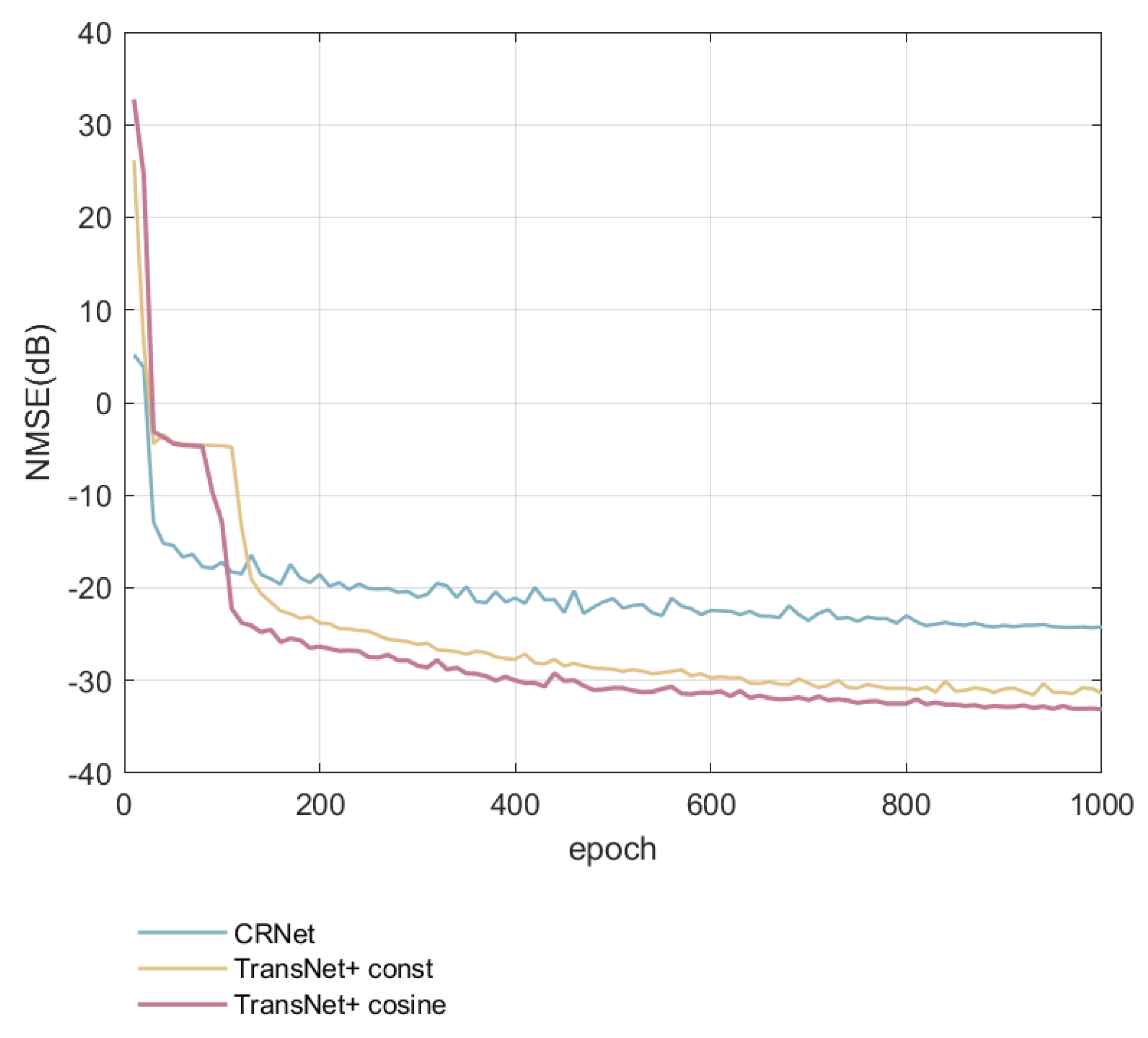
5. Simulation Results and Analysis

For comparison purposes, the CSI matrices dataset generated by COST 2100 [38] used in most DL-based CSI feedback studies is also used in this paper. The dataset contains channel matrices from indoor and outdoor scenarios, working at 5.3 GHz and 300 MHz, respectively. The number of transmitting antennas is set as $N_{\mathrm{t}}=32$ and the number of subcarriers is $N_{\mathrm{c}}=1024$. In the angular-delay domain, $N_{\mathrm{c}}$ reduces to $N_{\mathrm{a}}=32$ after truncation. As mentioned before, we adjust the dimension of TransNet+ $d_{\mathrm{model}}$ to 64 and optimize the number of attention heads $n_{\mathrm{head}}$ to 4. The training, validation, and testing datasets include 100,000, 30,000, and 20,000 matrices, respectively. We perform the accuracy evaluation by normalization mean square error (NMSE) following

$$\mathrm{NMSE}=\mathrm{E}\left\{\frac{{∥{\mathbf{H}}_a-{\widehat{\mathbf{H}}}_a∥}_2^2}{{∥{\mathbf{H}}_a∥}_2^2}\right\}$$

(9)

The model is built on PyTorch 1.12.0 (CUDA 10.2) and trained on a NVIDIA TITAN V GPU. The batch size is set as 200 and the training epoch is set as 1000. The warm-up aided cosine annealing training scheme is used to enable the model to learn higher resolution features. The maximum learning rate during training is $2\times {10}^{-4}$.

Table 1. NMSE (dB) and FLOPs comparison between TransNet+ and other methods based on attention mechanism.

Methods	Attention-CsiNet			LSTM-Attention CsiNet			SALDR			CsiFormer			TransNet			TransNet+
$\mathbf{\eta }$	in	out	FLOPs	in	out	FLOPs	in	out	FLOPs	in	out	FLOPs	in	out	FLOPs	in	out	FLOPs
1/4	−20.29	−10.43	24.72 M	−22.00	−10.20	∖	∖	∖	∖	∖	∖	∖	−32.38	−14.86	35.72 M	−33.12	−15.80	35.65 M
1/8	∖	∖	22.62 M	∖	∖	∖	−21.02	−9.35	141.57 M	∖	∖	∖	−22.91	−9.99	34.70 M	−23.47	−9.86	34.60 M
1/16	−10.16	−6.11	21.58 M	−11.00	−5.80	∖	−15.02	−5.96	141.12 M	∖	∖	∖	−15.00	−7.82	34.14 M	−15.70	−7.88	34.08 M
1/32	−8.58	−4.57	21.05 M	−8.80	−3.70	∖	−10.65	−3.79	140.87 M	−9.32	−3.51	5.41 M	−10.49	−4.13	33.88 M	−11.98	−4.87	33.82 M
1/64	−6.32	−3.27	20.79 M	−7.20	−2.40	∖	−7.80	−2.37	140.74 M	−6.85	−2.25	5.54 M	−6.08	−2.62	33.75 M	−7.99	−3.07	33.69 M

\ means the data is not presented in the corresponding paper.

shows the performance of CSI feedback schemes that have used the attention mechanism so far mentioned in [39] compared to the scheme proposed in our work. This makes sense because most networks based on attention mechanisms have achieved good results, especially TransNet achieved SOTA in most scenarios and at most compression rates. The epoch and batch size of these attention-based methods are the same as that of our model. $\eta$ represents the compression rate. The size of TransNet+ is in the middle compared to the other models, and this is acceptable because the FLOPs are not a hindrance compared to the exceptional CSI recovery accuracy attained by our model.

The data marked in bold is the data with the smallest NMSE at each compression rate. As shown in Table 1, TransNet+ obtains the best results at almost every compression ratio. TransNet+ performs better indoors than the model does outdoors. To be specific, NMSE of TransNet+ decreases by 0.74 dB, 0.56 dB, 0.70 dB, 1.49 dB, and 1.91 dB or 15.67%, 12.10%, 14.89%, 29.04%, and 35.58% with $\eta$ changing from 1/4 to 1/64 compared to TransNet. We observe that TransNet+ improves the performance of TransNet in particular at high compression ratios which is one of TransNet’s major limitations. In outdoor scenarios, TransNet+ also makes some progress in NMSE performance at $\eta =1/4,1/16,1/32$.

In the primary experiments of our work, we set the $n_{\mathrm{head}}$ as 4.

Table 2. NMSE(dB) for different $n_{\mathrm{head}}$ of the multi-head attention layer.

$\mathit{\eta }$	FLOPs	${\mathit{n}}_{\mathbf{head}}=1$	${\mathit{n}}_{\mathbf{head}}=2$	${\mathit{n}}_{\mathbf{head}}=4$	${\mathit{n}}_{\mathbf{head}}=8$
1/4	35.652 M	*	−29.42	−30.58	−7.58
1/8	34.603 M	−22.28	−22.83	−22.47	−22.75
1/16	34.079 M	−15.73	−15.90	−15.80	−16.09
1/32	33.817 M	−11.55	−11.06	−11.81	−10.98
1/64	33.686 M	−7.46	−5.91	−6.91	−6.65

* means the data does not converge during training.

justifies this choice by listing the performance of the model under different $n_{\mathrm{head}}$. The simulation is carried out in indoor scenarios. The epoch is set as 400 since the model tends to stabilize and the NMSE decreases at a noticeably slower rate after 400 epochs. With the result after 400 epochs, we can exclude some undesirable $n_{\mathrm{head}}$. For instance, the convergence property when $\eta =1/4$ is poor when $n_{\mathrm{head}}$ is 8. When $\eta$ equals 1/4 or 1/64, the NMSE performance reduces by more than 1 dB when $n_{\mathrm{head}}$ changes from 2 to 4. The network obtains the best results when $\eta =1/4,1/32$ with $n_{\mathrm{head}}=4$. The gaps between the results for $n_{\mathrm{head}}=4$ and the best results at the other three compression ratios are merely 0.36 dB, 0.29 dB, and 0.55 dB, respectively. In terms of overall performance, this gap is too minor to be taken into account. In general, the optimal number of attention heads is a balance between computational cost, number of parameters, and performance on accuracy. The model will reach a balance at a certain number of attention heads when the compression ratio is different. All we can do is select the number of attention heads that performs well at all compression ratios. Therefore, $n_{\mathrm{head}}$ selected in our network is 4 for both considerations of stability and recovery accuracy.

In Figure 4, we compare the NMSE of CRNet and TransNet+ with the cosine training scheme and TransNet+ with a constant learning rate. After 100 epochs, our model outperforms CNN-based CRNet by a large margin. The results of the first 400 epochs indicate that TransNet+ with the cosine training scheme converges faster. Meanwhile, the results of the remaining epochs demonstrate that TransNet+ has superior recovery accuracy. This is because the warm-up cosine training scheme has a high learning rate at the early stage, which makes the model learn features rapidly and accelerate the training speed, and a lower learning rate at the later stage, allowing the model to learn high-resolution features to obtain better feedback quality. Simultaneously, the higher dimensional feature representation also contributes to the improvements in recovery accuracy.

6. Discussion

For broader comparison and higher credibility, the NMSE performance of our work is compared with the best performance of all models concluded by [39], not only those introducing the attention mechanism. MRFNet [40] achieves the best NMSE = −15.95 dB in outdoor scenarios at $\eta =1/4$. The gap between our model and MRFNet is only 0.15 dB. The NMSE of ENet [41] is −11.20 dB in indoor scenarios when $\eta$ equals 1/32, which has been surpassed by our model. In outdoor scenarios, a neural network named CsiNet+DNN proposed in [42] gets remarkable results at the expense of extremely high computational overhead. Compared to TransNet+ and other attention models, the deployment resource overhead of CsiNet+DNN may be significantly larger. In the remaining cases, TransNet+ outperforms all the other networks.

Although TransNet+ achieves higher recovery accuracy, which reaches SOTA for almost all scenarios, practical deployment issues are not within the scope of the study. The majority of research in this field relies on simulations where CSI samples are readily generated using channel modeling software such as COST 2100, facilitating the acquisition of extensive CSI data for model training purposes. However, the implementation of DL-based CSI feedback in real wireless systems necessitates consideration of data gathering and online training. This necessity arises primarily for two reasons. Firstly, during wireless communication, the UE may not have the opportunity to collect a sufficient quantity of CSI samples. Secondly, the actual propagation environment can undergo changes, particularly in mobile wireless settings, rendering the network parameters trained on static data inadequate for adapting to dynamic real-time channels. This is one of the significant directions for our future research.

7. Conclusions

In this paper, a network called TransNet+ based on the Transformer architecture is proposed. We not only extend the ability of the model to focus on long-range dependency, but also adopt high-dimensional feature representation to improve the feedback quality. Additionally, the warm-up cosine training scheme is introduced for quicker convergence and stronger capability to learn CSI features. Numerical results indicate that, compared to other attention mechanism-based models, our model consistently achieves the best results at almost every compression ratio, especially in indoor low-noise environments. Despite the superior performance achieved by TransNet+ in our current work, the network still requires improvements for practical applications in the future. For example, codeword quantization needs to be considered to simulate actual communication scenarios. Moreover, collecting CSI datasets in the real model training process and developing methods to mitigate network performance degradation in frequently changing environments caused by offline training will become the direction of future research.

References

1. Han, F.; Zeng, J.; Zheng, L.; Zhang, H.; Wang, J. Sensing and Deep CNN-Assisted Semi-Blind Detection for Multi-User Massive MIMO Communications. Remote Sens. 2024, 16, 247. [Google Scholar] [CrossRef]
2. Lin, W.-Y.; Chang, T.-H.; Tseng, S.-M. Deep Learning-Based Cross-Layer Power Allocation for Downlink Cell-Free Massive Multiple-Input–Multiple-Output Video Communication Systems. Symmetry 2023, 15, 1968. [Google Scholar] [CrossRef]
3. Pan, F.; Zhao, X.; Zhang, B.; Xiang, P.; Hu, M.; Gao, X. CSI Feedback Model Based on Multi-Source Characterization in FDD Systems. Sensors 2023, 23, 8139. [Google Scholar] [CrossRef]
4. Liu, Q.; Sun, J.; Wang, P. Uplink Assisted MIMO Channel Feedback Method Based on Deep Learning. Entropy 2023, 25, 1131. [Google Scholar] [CrossRef] [PubMed]
5. Riviello, D.G.; Tuninato, R.; Zimaglia, E.; Fantini, R.; Garello, R. Implementation of Deep-Learning-Based CSI Feedback Reporting on 5G NR-Compliant Link-Level Simulator. Sensors 2023, 23, 910. [Google Scholar] [CrossRef] [PubMed]
6. Sun, Q.; Zhao, H.; Wang, J.; Chen, W. Deep Learning-Based Joint CSI Feedback and Hybrid Precoding in FDD mmWave Massive MIMO Systems. Entropy 2022, 24, 441. [Google Scholar] [CrossRef] [PubMed]
7. Naser, M.A.; Abdul-Hadi, A.M.; Alsabah, M.; Mahmmod, B.M.; Majeed, A.; Abdulhussain, S.H. Downlink Training Sequence Design Based on Waterfilling Solution for Low-Latency FDD Massive MIMO Communications Systems. Electronics 2023, 12, 2494. [Google Scholar] [CrossRef]
8. Li, Q.; Zhang, A.; Liu, P. A novel CSI feedback approach for massive MIMO using LSTM-attention CNN. IEEE Access 2020, 8, 7295–7302. [Google Scholar] [CrossRef]
9. Manasa, B.M.R.; Pakala, V.; Chinthaginjala, R.; Ayadi, M.; Hamdi, M.; Ksibi, A. A Novel Channel Estimation Framework in MIMO Using Serial Cascaded Multiscale Autoencoder and Attention LSTM with Hybrid Heuristic Algorithm. Sensors 2023, 23, 9154. [Google Scholar] [CrossRef] [PubMed]
10. Bi, X.; Li, S.; Yu, C. A novel approach using convolutional transformer for massive MIMO CSI feedback. IEEE Wirel. Commun. Lett. 2022, 11, 1017–1021. [Google Scholar] [CrossRef]
11. Cui, Y.; Guo, A.; Song, C. TransNet: Full attention network for CSI feedback in FDD massive MIMO system. IEEE Wirel. Commun. Lett. 2022, 11, 903–907. [Google Scholar] [CrossRef]
12. Lu, Z.; Wang, J.; Song, J. Multi-resolution CSI feedback with deep learning in massive MIMO system. In Proceedings of the 2020 IEEE International Conference on Communications (ICC), Dublin, Ireland, 7–11 June 2020; pp. 1–6. [Google Scholar]
13. Chen, J.; Mei, M. Numerical Analysis of Low-Cost Recognition of Tunnel Cracks with Compressive Sensing along the Railway. Appl. Sci. 2023, 13, 13007. [Google Scholar] [CrossRef]
14. Wen, C.K.; Shih, W.T.; Jin, S. Deep learning for massive MIMO CSI feedback. IEEE Wirel. Commun. Lett. 2018, 7, 748–751. [Google Scholar] [CrossRef]
15. Sharma, S.; Yoon, W. Energy Efficient Power Allocation in Massive MIMO Based on Parameterized Deep DQN. Electronics 2023, 12, 4517. [Google Scholar] [CrossRef]
16. Zhang, Y.; Luo, Z. A Review of Research on Spectrum Sensing Based on Deep Learning. Electronics 2023, 12, 4514. [Google Scholar] [CrossRef]
17. Lu, C.; Xu, W.; Jin, S.; Wang, K. Bit-level optimized neural network for multi-antenna channel quantization. IEEE Wirel. Commun. 2019, 9, 87–90. [Google Scholar] [CrossRef]
18. Ji, S.; Li, M. CLNet: Complex input lightweight neural network designed for massive MIMO CSI feedback. IEEE Wirel. Commun. Lett. 2021, 10, 2318–2322. [Google Scholar] [CrossRef]
19. Lu, Z.; Wang, J.; Song, J. Binary neural network aided CSI feedback in massive MIMO system. IEEE Wirel. Commun. Lett. 2021, 10, 1305–1308. [Google Scholar] [CrossRef]
20. Guo, J.; Wen, C.-K.; Jin, S.; Li, G.Y. Convolutional neural network based multiple-rate compressive sensing for massive MIMO CSI feedback: Design, simulation, and analysis. IEEE Trans. Wirel. Commun. 2020, 19, 2827–2840. [Google Scholar] [CrossRef]
21. Wang, T.; Wen, C.; Jin, S.; Li, G.Y. Deep learning-based CSI feedback approach for time-varying massive MIMO channels. IEEE Wirel. Commun. Lett. 2019, 8, 416–419. [Google Scholar] [CrossRef]
22. Cai, Q.; Dong, C.; Niu, K. Attention model for massive MIMO CSI compression feedback and recovery. In Proceedings of the 2019 IEEE Wireless Communications and Networking Conference (WCNC), Marrakesh, Morocco, 15–18 April 2019; pp. 1–5. [Google Scholar]
23. Song, X.; Wang, J.; Wang, J. SALDR: Joint self-attention learning and dense refine for massive MIMO CSI feedback with multiple compression ratio. IEEE Wirel. Commun. Lett. 2021, 10, 1899–1903. [Google Scholar] [CrossRef]
24. Hong, S.; Jo, S.; So, J. Machine learning-based adaptive CSI feedback interval. ICT Express 2022, 8, 544–548. [Google Scholar] [CrossRef]
25. Liu, Z.; Zhang, L.; Ding, Z. Exploiting bi-directional channel reciprocity in deep learning for low rate massive MIMO CSI feedback. IEEE Wirel. Commun. Lett. 2019, 8, 889–892. [Google Scholar] [CrossRef]
26. Wang, J.; Gui, G.; Ohtsuki, T. Compressive sampled CSI feedback method based on deep learning for FDD massive MIMO systems. IEEE Trans. Commun. 2021, 69, 5873–5885. [Google Scholar] [CrossRef]
27. Mashhadi, M.B.; Yang, Q.; Gunduz, D. Distributed deep convolutional compression for massive MIMO CSI feedback. IEEE Trans. Wirel. Commun. 2020, 20, 2621–2633. [Google Scholar] [CrossRef]
28. Liu, Z.; del Rosario, M.; Ding, Z. A Markovian model-driven deep learning framework for massive MIMO CSI feedback. IEEE Trans.Wirel. Commun. 2022, 21, 1214–1228. [Google Scholar] [CrossRef]
29. Guo, J.; Wen, C.K.; Jin, S. CAnet: Uplink-aided downlink channel acquisition in FDD massive MIMO using deep learning. IEEE Trans. Commun. 2021, 70, 199–214. [Google Scholar] [CrossRef]
30. Chen, M.; Guo, J.; Wen, C.K. Deep learning-based implicit CSI feedback in massive MIMO. IEEE Trans. Commun. 2021, 70, 935–950. [Google Scholar] [CrossRef]
31. Qing, C.; Cai, B.; Yang, Q. Deep learning for CSI feedback based on superimposed coding. IEEE Access 2019, 7, 93723–93733. [Google Scholar] [CrossRef]
32. Xu, D.; Huang, Y.; Yang, L. Feedback of downlink channel state information based on superimposed coding. IEEE Commun. Lett. 2007, 11, 240–242. [Google Scholar] [CrossRef]
33. Guo, J.; Chen, T.; Jin, S. Deep learning for joint channel estimation and feedback in massive MIMO systems. Digit. Commun. Netw. 2023. [Google Scholar] [CrossRef]
34. Jang, J.; Lee, H.; Hwang, S. Deep learning-based limited feedback designs for MIMO systems. IEEE Wirel. Commun. Lett. 2019, 9, 558–561. [Google Scholar] [CrossRef]
35. Ye, H.; Gao, F.; Qian, J. Deep learning-based denoise network for CSI feedback in FDD massive MIMO systems. IEEE Commun. Lett. 2020, 24, 1742–1746. [Google Scholar] [CrossRef]
36. Vaswani, A.; Shazeer, N.; Parmar, N.; Uszkoreit, J.; Jones, L.; Gomez, A.N. Attention is all you need. In Proceedings of the 31st International Conference on Neural Information Processing Systems (ICONIP), Long Beach, CA, USA, 4–9 December 2017; Volume 30, pp. 5998–6008. [Google Scholar]
37. Xue, J.; Chen, X.; Chi, Q.; Xiao, W. Online Learning-Based Adaptive Device-Free Localization in Time-Varying Indoor Environment. Appl. Sci 2024, 14, 643. [Google Scholar] [CrossRef]
38. Liu, L.; Oestges, C.; Poutanen, J.; Haneda, K.; Vainikainen, P.; Quitin, F. The cost 2100 MIMO channel model. IEEE Wirel. Commun. 2012, 19, 92–99. [Google Scholar] [CrossRef]
39. Guo, J.; Wen, C.K.; Jin, S. Overview of deep learning-based CSI feedback in massive MIMO systems. IEEE Trans. Commun. 2022, 70, 8017–8045. [Google Scholar] [CrossRef]
40. Hu, Z.; Guo, J.; Liu, G.; Zheng, H.; Xue, J. MRFNet: A deep learning-based CSI feedback approach of massive MIMO systems. IEEE Commun. Lett. 2021, 25, 3310–3314. [Google Scholar] [CrossRef]
41. Sun, Y.; Xu, W.; Liang, L.; Wang, N.; Li, G.Y.; You, X. A lightweight deep network for efficient CSI feedback in massive MIMO systems. IEEE Wirel. Commun. Lett. 2021, 10, 1840–1844. [Google Scholar] [CrossRef]
42. Zhang, Y.; Zhang, X.; Liu, Y. Deep learning based CSI compression and quantization with high compression ratios in FDD massive MIMO systems. IEEE Wirel. Commun. Lett. 2021, 10, 2101–2105. [Google Scholar] [CrossRef]
Figure 1. The structure of the encoder and decoder of our network.
Applsci 14 01356 g001
Figure 2. The internal structure of a single multi-head attention layer with n head = 4 . The second to fourth sets of Q , K and V have also been multiplied by three different sets of W Q , W K and W V , which is omitted in the figure. The dotted arrow indicates that V is not processed by the softmax layer.
Applsci 14 01356 g002
Figure 3. The trend of learning rate when utilizing the warm-up cosine training scheme and a constant learning rate.
Applsci 14 01356 g003
Figure 4. The trends of NMSE during testing at η = 1 / 4 in indoor scenarios.
Applsci 14 01356 g004