Article

Petrophysical Property Prediction from Seismic Inversion Attributes Using Rock Physics and Machine Learning: Volve Field, North Sea

by
Doyin Pelemo-Daniels
* and
Robert R. Stewart
Department of Earth and Atmospheric Sciences, University of Houston, Science and Research Building 1, 3507 Cullen Blvd, Room 312, Houston, TX 77204-5007, USA
*
Author to whom correspondence should be addressed.
Appl. Sci. 2024, 14(4), 1345; https://doi.org/10.3390/app14041345
Submission received: 6 November 2023 / Revised: 12 December 2023 / Accepted: 14 December 2023 / Published: 6 February 2024
(This article belongs to the Section Earth Sciences)

Abstract

:
An accurate petrophysical model of the subsurface is essential for resource development and CO2 sequestration. We present a new workflow that provides a high-resolution estimate of petrophysical reservoir properties using seismic data with rock physics modeling and machine-learning techniques (i.e., deep learning neural networks). First, we compare the sequential prediction of the following petrophysical attributes: mineralogy, porosity, and fluid saturation, with the simultaneous prediction of all of the properties using the Volve field in the Norwegian North Sea as an example. The workflow shows that the sequential prediction produces a more efficient and accurate classification of petrophysical properties (the RMS error between the predicted and the original seismic trace is 50% smaller for the sequential compared to the simultaneous procedure). Next, the seismic amplitude response of the reservoirs was studied using rock physics modeling and amplitude versus offset (AVO) analysis to distinguish the different lithologies and fluid types. To ascertain the optimal hydrocarbon production areas, we performed Bayesian seismic inversion and applied machine learning to estimate the petrophysical properties. We examined how porosity, Vclay, and fluid variations affect the elastic properties. In Poisson’s ratio versus the P-wave impedance domain, a 10% porosity increase decreases the acoustic impedance (AI) by 30%, while a 20% Vclay decrease increases the AI by 12%. The Utsira Formation in the Volve field (5 km north of the Sleipner Øst field) was evaluated as a potential CO2 geological storage unit using Gassmann fluid substitution and seismic modeling. We look to assess the elastic property variation caused by CO2 saturation changes for monitoring purposes and simulate the effect. In the first 10% CO2 substitution, the P-wave velocity decrease is 12%, a subtle effect is observed for higher CO2 saturation values, and S-wave velocity (Vs) increases with CO2 saturation. Our analysis aspires to assist future reservoir studies and CO2 sequestration in similar fields.

1. Introduction

Inferring petrophysical properties from seismic data is a key step in reservoir characterization [1,2]. The 3D information, in conjunction with well-log data, provides crucial information for enhanced field development and exploration programs, as well as potential CO2 sequestration development. However, extracting petrophysical properties from seismic data is a complex inverse problem that integrates mathematical methods with physical relations like petrophysics, wave propagation, and rock physics [3]. Point-wise estimates of density (ρ), P-wave velocities (Vp), S-wave velocities (Vs), and impedances can be obtained through seismic inversion [4]. Nevertheless, uncertainty stems from the fact that many combinations of shear and acoustic impedance can result in equivalent rock properties. One approach to minimizing uncertainty or non-uniqueness is integrating rock physics and petrophysics models with seismic inversion results to estimate a unique 3D petrophysical property model [5].
Several researchers have attempted to estimate or enhance petrophysical properties through seismic inversion. In their works, [6,7,8] investigated the integrated approach of combining seismic inversion and attribute analysis, emphasizing their significance in reservoir characterization and the prediction of petrophysical properties. Ref. [9] is a review that explores the recent advancements in seismic reservoir characterization, with a focus on how refined seismic inversion techniques contribute to increased recovery factors. Ref. [10] delved into the application of machine-learning techniques to predict petrophysical properties from seismic data, providing valuable insights into the integration of data-driven approaches. Nevertheless, it is essential to acknowledge that, over time, there has been a continuous progression in research and analysis to enhance the prediction of petrophysical parameters through seismic inversion.
Recent research has demonstrated the effectiveness of neural networks and other machine-learning techniques in property estimation [11]. Ref. [12] is an evaluation of machine-learning methods for supervised lithology classification using geophysical data and shows that RandomForest and multilayer perception (MLP) yielded the highest accuracy. Also, other ML methods with better accuracy were applied to the classification of offshore wells. Furthermore, ML models have been applied to conventional well-log data to identify the shale lithofacies [13], deep convolutional neural network for seismic horizon tracking [14], and neural networks for the interpretation of 3D seismic structural data that aim to identify potential well site [15] models. These methods offer valuable support in mitigating risks by facilitating the development of precise subsurface models through efficient workflows [16]. It is safe to conclude that the ML methods have been applied to a wide range of geophysical data, and the level of accuracy has been proven to be replicable to newly generated data.
The application of these techniques proves to be suitable for enhancing existing petrophysical and rock physics workflows, thereby leading to improved result accuracy. While machine learning (ML) has shown promise in predicting petrophysical parameters, some of the major limitations and challenges associated with its application are the contexts of data quality and quantity. ML algorithms heavily rely on the quality and quantity of the training data. Limited or poor-quality data can lead to biased or inaccurate predictions. In this study, our objective is to contribute to this evolving research landscape by improving the accuracy and efficiency of predicting petrophysical parameters from seismic data by performing detailed rock physics diagnostics of well-log data (training data set) and also introduce a more efficient workflow to enhance our prediction.
The motivation for our study stems from the fact that petrophysical analyses from well logs are carried out sequentially. In traditional well-log analysis, we typically determine the volume of the rock types, porosity, and fluid saturation by using a sequential approach. The process involves computing the lithology first, followed by the porosity, and finally, the saturation using measured well-log data. Our research introduces an innovative workflow that leverages machine learning to predict petrophysical parameters from seismic data sequentially. From our seismic inversion, we obtain our impedance volume (acoustic (primary wave) impedance (AI) and shear wave impedance (SI) volumes). Using the AI and SI volumes, the algorithm predicts the lithology volume. Then, it is trained to incorporate the predicted lithology to estimate the porosity. Finally, by incorporating the predicted porosity, lithology, and measured logs, the algorithm predicts the saturation volume. We compare our results with an approach that simultaneously predicts all of the parameters at once from the seismic data. This new methodology aims to enhance the efficiency and accuracy of petrophysical analysis from seismic data.
The initial phase of this investigation is dedicated to constructing a comprehensive three-dimensional model encompassing key rock attributes, specifically porosity, lithology, and water saturation. Subsequently, machine learning is employed to predict the petrophysical parameters based on property measurements derived from analogous observations. In pursuit of this, we adopt the neural network approach, as implemented in [17], which establishes a relationship between input data and target properties, as highlighted by [18,19]. To achieve this objective, we establish a rock property model that bridges the gap between petrophysical properties and seismic rock properties, building upon the work of [20].
To facilitate this process, we first conduct a visual evaluation to assess the feasibility of differentiating lithologies, porosity levels, and fluid types by cross plotting various elastic attributes. This assessment provides essential information regarding the optimal elastic property combinations, the number of litho-classes for evaluation, and the adequacy of well-log data representation. This preliminary analysis assists in defining the cut-off values for reservoir parameters, including porosity, saturation, and clay volume, within various lithofluid classes.
Moreover, this work introduces an innovative workflow that employs machine learning for the prediction of petrophysical parameters from seismic data. By utilizing rock physics modeling, we identify the most effective combination of rock properties to distinguish the primary reservoir quality responses from background trends.
Given the increasing interest in carbon dioxide (CO2) sequestration, the study’s final phase encompasses CO2 modeling to evaluate the Utsira Formation in the Volve area as a viable CO2 geological storage location. This phase involves fluid substitution modeling utilizing well-log data to quantify the effects of CO2 injection. Synthetic seismograms are generated for various CO2 saturation levels, and Gassmann equations are applied to calculate changes in the P-wave and S-wave velocity. Synthetic stack and gather sections are created, covering a range from 0% to 100% CO2 saturation in 10% increments, with the parameters adjusted at each step. This comprehensive model provides insights into the seismic response to CO2 saturation and the evolution of the injection process.

2. Background—Study Areas
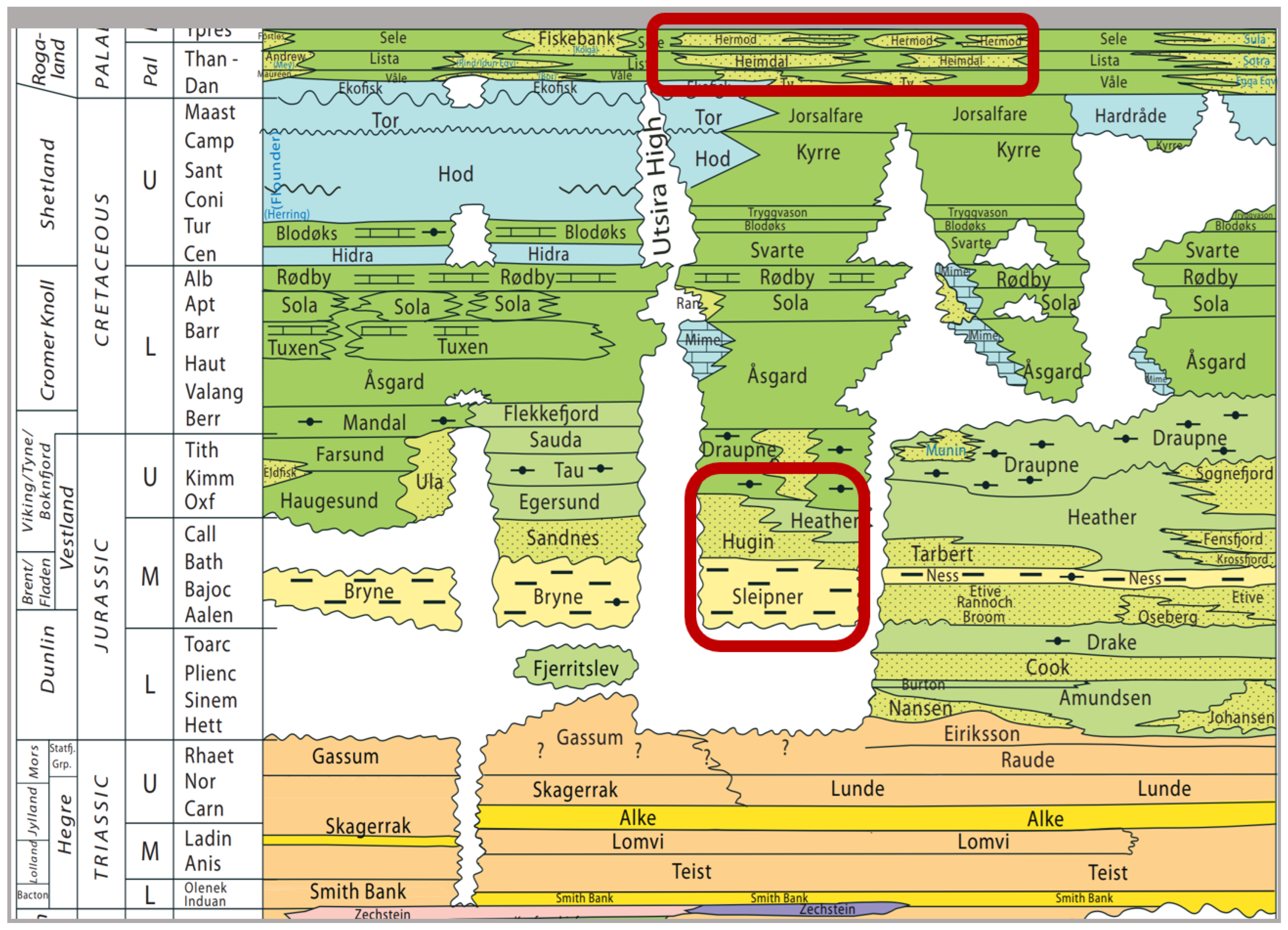
The study areas are the Volve and Sleipner fields, which are in the Norwegian North Sea (Figure 1).

2.1. Geology

The Volve oil field was discovered in the Norwegian North Sea in 1993 and was approved for development in 2005. The field was productive from 2008 to 2016 and achieved 63 million barrels of cumulative oil and minimum production rates of 56,000 bopd [22,23]. The main reservoir of interest is the Hugin Formation sandstone. In addition, the Heimdal, Utsira, and Skagerrak Sands are considered to be secondary reservoirs (Figure 2). The Hugin and Heimdal reservoirs are heavily faulted, particularly in the western area, most possibly caused by regional extension and salt tectonics [24].
The Utsira Sand is a regional saline aquifer. It is a part of the late Cenozoic post-rift succession in the North Sea Basin. The stratigraphical lap-out establishes its eastern and western boundaries. At the same time, it passes laterally into finer-grained terrain to the southwest. It also occupies a narrow, deepening channel to the north.
The top Utsira Sand surface ranges in total depth from 550 to 1500 m near the Sleipner and Volve fields. The Utsira Sand’s base is more structurally complex, with several mounds interpreted as mud diapirs. The mud diapirism is linked to local faults at the reservoir’s base, but it does not appear to affect the reservoir’s upper levels or caprock [25]. The Utsira reservoir’s overburden is approximately 700 m thick. The primary reservoir caprock is basin-restricted mudstone that extends more than 50 km west and 40 km east of the Sleipner CO2 injection area [25].
Figure 2. Chart showing the lithostratigraphic column of the North Sea [26]. The highlighted sections in red show the reservoirs of interest: the Heimdal, Hugin, and Skagerrak Sands.
Applsci 14 01345 g002

2.2. Reservoir Characteristics

The Hugin Formation is a sequence of sandstones that were deposited in an environment characterized by shallow water and tidal activity. This sequence has a significant lateral extent. The reservoir is relatively clean and homogeneous. Quartz, clay, and mica predominate as the primary mineralogy components of the sandstones [22]. Studies of the fluid in the reservoirs have revealed that the oil found in the Volve field originated in the Sleipner Graben region, located in the northwest part of the field, approximately 10 million years ago. The oil then moved into the Volve reservoir structure. In the upper section of the Draupne Formation, type II kerogen was found, confirmed by a high gamma-ray response, which led to the hypothesis that this could be the source rock [22]. The Volve field oil is under-saturated with 27–29° API oil, with a gas/oil ratio of 111–157 Sm3/Sm3. It contains between 2% and 6% asphaltenes, as well as sulfur and aromatic components in high concentrations [26].
Regarding well logs, the Utsira Sand can be distinguished by its top and bottom layers, and the percentage of clean sand that makes up the reservoir unit typically exceeds 70 percent. The quasi-proportion comprises thin mudstones, which have an average thickness of approximately one meter and are expressed as peaks on the gamma-ray and resistivity logs. The ‘five-meter mudstone’ is a thicker and more laterally persistent bed than the others, and it differentiates the uppermost sand unit from the main reservoir below it. It has been demonstrated that the mudstone layers present within the reservoir sand act as substantial permeability barriers, which significantly influence the amount of CO2 that migrates through the reservoir [27].

3. Methodology

Both pre-stack and post-stack seismic volumes provided by Equinor [28], along with a suite of logs from 13 wells, core data, and well reports, are incorporated into this work. The study began by performing quality control (QC) assessments on seismic data. This involves essential checks such as assessing the following: fold coverage, stacking quality, amplitude and phase spectra, geometry, signal-to-noise ratio, data consistency, migration effectiveness, well-tie correlation, sample rate, and dominant frequency. These checks are crucial for ensuring the seismic data’s reliability, accuracy, and suitability, facilitating improved interpretation and inversion results by addressing issues related to subsurface sampling, signal clarity, and frequency content. The seismic data have a sample rate of 4 ms and a Nyquist frequency of 125 Hz. The well-seismic tie correlation shows an average correlation coefficient of about 0.82.
Next, we conduct a thorough quantitative examination of the well-log and core data. After that, a set of physical relations is calibrated to ascertain the viability of obtaining petrophysical parameters from the seismic inversion results. This calibration involves porosity, saturation, and mineralogy estimations. The well logs are also analyzed to determine the most significant reservoir zones of interest (ZoI). These zones are then analyzed for lithology and fluid saturation with the help of petrophysical models.
To calibrate a reservoir-dependent rock physics model appropriate for the Volve field, rock physics diagnostics (RPD) are then conducted. After that, using the rock models created during the RPD stage, we perform perturbational modeling to create potential reservoir scenarios. Finally, we evaluate the seismic responses and amplitude versus offset (AVO) signatures of the different rock physics perturbations. Synthetic gathers are generated for each well based on different model scenarios.
The second part of this work entails changes in the reflection angle by incorporating rock physics modeling and the synthetic seismic analysis results. Lastly, we perform seismic inversion and apply machine learning to predict clay volume, porosity, and water saturation. These results indicate that the optimal hydrocarbon production areas correlate reasonably well with the actual production values.

3.1. Rock Physics Workflow

The rock physics workflow entails geophysical well-log analyses, rock physics diagnostics, perturbation, and synthetic seismogram modeling.

3.1.1. Geophysical Well-Log Analyses

The first step is to edit the logs and remove erroneous data. In this instance, a trend is established by plotting each log against depth. Data values that significantly deviate from this trend are treated as outliers and are edited accordingly. Next, qualitative and quantitative methods are used to identify hydrocarbon-bearing reservoirs (Figure 3). In the qualitative analysis, the well logs are scanned for indications of hydrocarbon reservoirs, such as low gamma-ray responses and high resistivity. The quantitative approach also involves computing parameters like lithology volume, water saturation, and effective porosity. Using rock physics, reservoir zones were identified and analyzed. Volume concentrations are determined from a statistical solution utilizing the neutron, density, photoelectric factor, compressional, and shear velocities. The mass-balance equation is used to compute the porosity from the density. Archie’s equations are used to compute the water saturation (Sw). Sands are characterized as having Vquartz greater than 60%, oil sands as having Vquartz greater than 60% and Sw less than 60%, and shale as having Vclay greater than 60%. Overall, the quartz volume appears consistent in all of the wells, with an average of 70%.

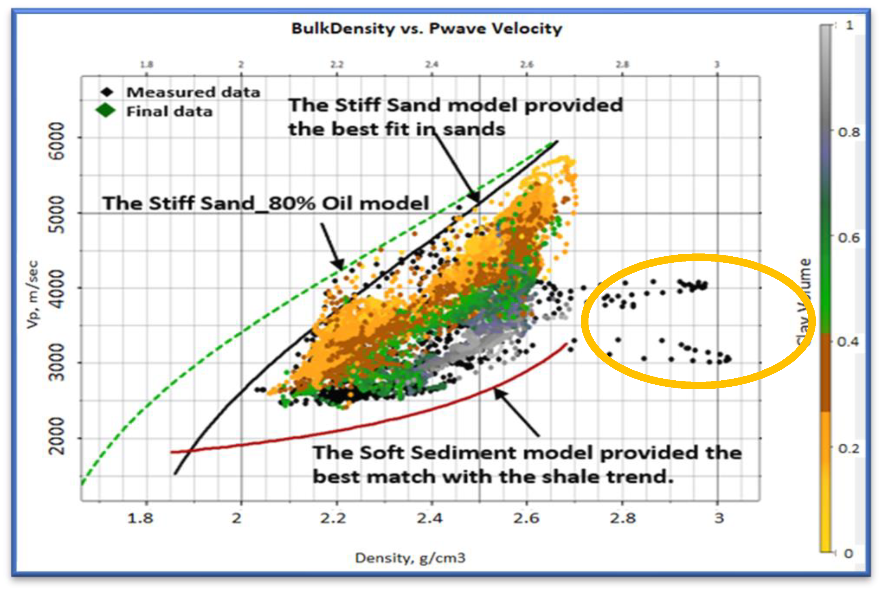
3.1.2. Rock Physics Diagnostics

Hertz-Mindlin’s contact theory and the modified Hashin-Strikman lower bound are used to derive theoretical estimations of the effective elastic constants of unconsolidated sand [29]. First, the aggregate’s shear and effective bulk moduli are calculated, assuming that all grains are spherical and organized in a random pack with a porosity of 0.36. Next, the modified Hashin-Strikman lower bound is used to find the effective elastic moduli at a decreased porosity. Suspension-like rocks are best described with this bound. The Ref. [30] equation is used to introduce the impact of pore fluid. The stiff sand model estimates bulk modulus (K) and shear modulus (u) from the porosity and fluid characteristics using the HMHS “contact cement” sand model of [5]. Using elasticity equations, Vp and Vs are calculated from K and u [31]. The HM unconsolidated sphere pack model determines the high porosity velocity limit. At the maximum porosity level, a higher coordination equals a stiffer pack and, as a result, a higher velocity. In ref. [32], the authors devised a method for predicting Vs in porous rocks that is now widely used.
The rock physics models (RPM) that best fit the measured data were identified. These models establish a deterministic relationship between reservoir parameters (such as minerals, fluids, porosity, and geometry) and elastic properties (i.e., P-wave velocity Vp, S-wave velocity Vs, and density). We use these models to adjust the Vp, Vs, and density when they are missing or have inaccurate measurements. More importantly, we modify the elastic response for changes in porosity caused by compaction.
We have utilized granular models to predict the P-wave velocity and response due to the clastic nature of the environment. Figure 4 and Figure 5 illustrate that the stiff sand model better predicts the response of sand-rich sediments, while the soft sediment model better predicts the response of shales [33]. The modified [34] relationship is most suitable for Vs prediction, with a correlation coefficient as high as 0.9.

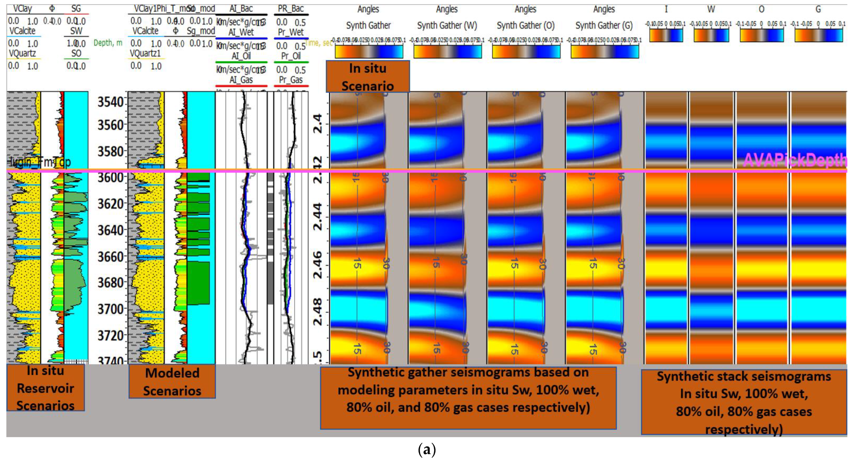
3.1.3. Perturbational and Synthetic Modeling

Perturbation modeling is an important component of seismic attribute investigations because it allows predictions of seismic responses for various fluid scenarios [35]. In this study, the lithology, porosity, and fluid modeling on the Hugin Sands are performed using the [36] equations. This was accomplished to see what combination of rock attributes might be used to distinguish the reservoir responses from their background trend and to see if the different lithofacies in the Volve field could be distinguished.
For the perturbational modeling scenarios, we assume the following five cases: the first is the in situ scenario, in which we assume the in situ lithology and porosity and only change the fluid scenarios; the second is a low porosity scenario, in which we reduce the porosity by ten porosity units; the third is a shaly reservoir scenario, in which we increase the clay content by 20%; in the fourth case we simultaneously reduce the porosity by ten porosity units; and, finally, in the fifth case, we simultaneously increase the porosity by ten porosity units while decreasing the clay content by 20%, followed by fluid substitution modeling.

Fluid Substitution and Synthetic Modeling

Gassmann equations are used to perform all fluid substitution cases in the sands during fluid modeling [30]. The hydrocarbon scenario is assumed to be 80 percent hydrocarbon and 20 percent brine, whereas the wet scenario is assumed to be 100 percent brine. To investigate the signatures of the in situ and modeled cases, synthetic gathers are generated. Using the wavelet extracted from the seismic data and upscaled elastic curves, full-offset synthetic seismograms with zero offsets are created and smoothed using Backus windows of varying window sizes based on velocities, and, for the wavelet, the elastic curves are then upscaled to a higher resolution.

Vclay Modeling

The Vclay modeling process entails altering the clay volume for each scenario, estimating the elastic logs (velocities and densities), and taking into account the new lithology using established rock physics models. First, we change the porosity scenarios for the porosity modeling and then compute the density using the new total porosity. Vp and Vs are then estimated using the calibrated rock physics models. The first thing we perform when modeling porosity is adding matrix porosity to the rock. After that, we change the fluid in place (approximately 80% oil and 20% brine) to 100% brine. Each distinct alteration in porosity is equivalent to a specific percentage of the total porosity of the in situ matrix.

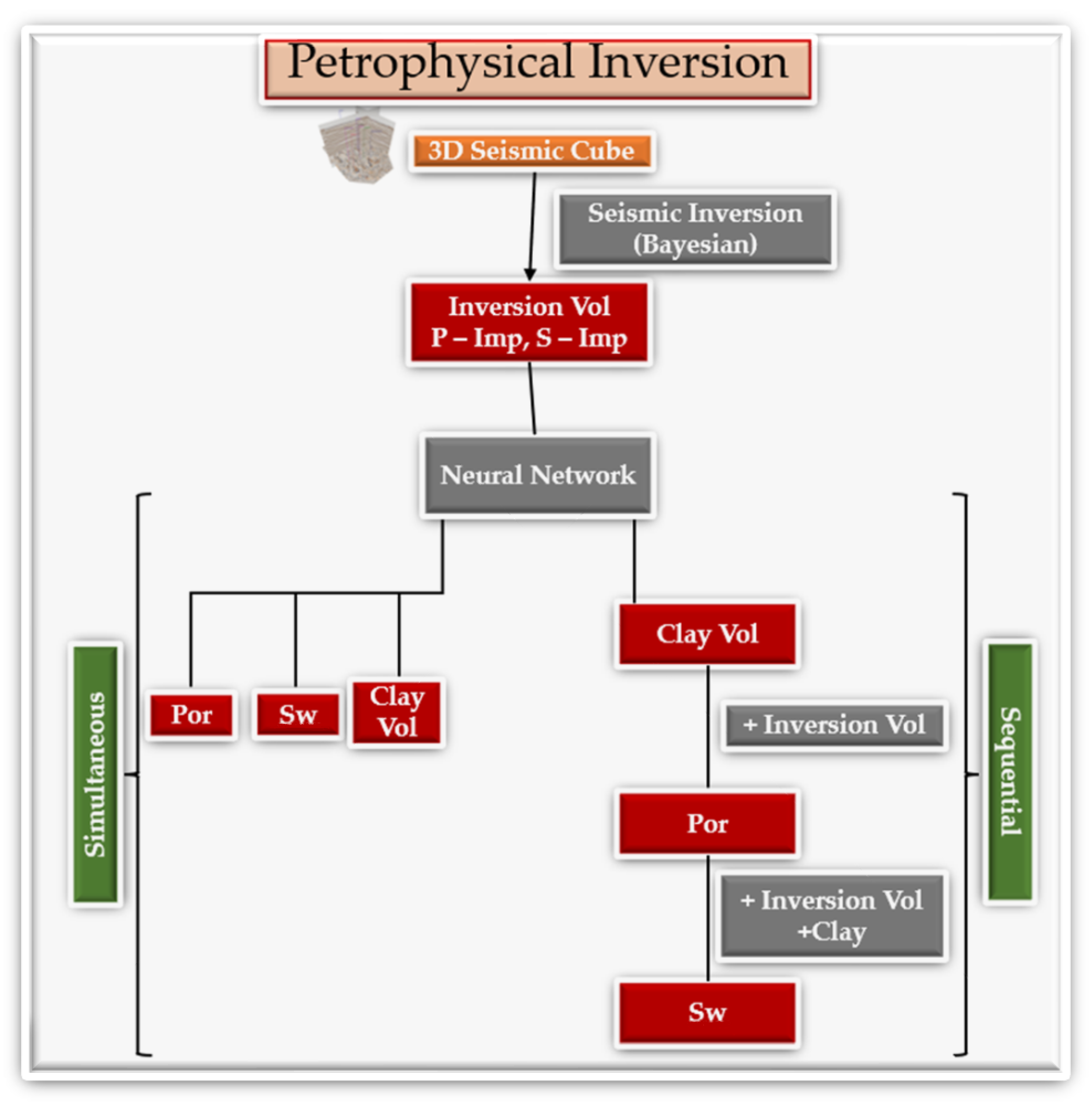
3.1.4. Petrophysical Seismic Inversion

The linearized Bayesian AVO inversion, as described in [37], formulates the challenge within a probabilistic and statistical framework. In this approach, prior knowledge sourced from independent references, such as well-log data, is integrated with AVO equations or the likelihood function. Reservoir coupling information, serving as prior data, plays a pivotal role in constraining the AVO inverse problem while operating under the assumption of a Gaussian probability density function.
“Equation (1) represents the forward linear model, where ‘dobs’ denotes the observed seismic data, G stands for the kernel matrix, W is a block diagonal matrix containing angle-dependent wavelets, C is a sparse matrix containing AVO coefficients, ‘m’ comprises the model parameters, and D serves as a derivative operator. In this context, ‘m’ takes the form of a column vector encompassing compressional wave velocity (Vp), shear wave velocity (Vs), and density ( ρ ). The likelihood function employed is the linearized version of the Aki and Richards equation [38].
d o b s = G m + N o i s e   a b
G = W   C   D   ( a b )
The utilization of linearized forward equations enhances computational efficiency within the Bayesian model. The three-term AVO equation characterizes the relationship between reflection amplitude and offset (angle). Equation (2) represents a continuous-time formulation of Aki and Richards’ equation, as detailed in [39].
R p p t , θ = C 1 θ , t t I n V p + C 2 θ , t t I n V s + C 3 θ , t t I n ρ
In this context, R p p refers to the offset-dependent compressional reflectivity and C 1 to C 3 represent the AVO coefficients, with θ denoting the offset angle.
Bayes’ theorem provides a mathematical framework for incorporating prior information related to the elastic parameters, including density, compressional, and shear wave properties, which are to be derived from the seismic data using the forward model (AVO equations). This approach allows for the generation of probabilistic estimates, facilitating the assessment of the uncertainties associated with these parameters.
The theorem can be expressed as follows:
Q m d = P d m P m P d
Here, Q m d represents the posterior distribution, which provides a probabilistic solution to the inverse problem; P d m denotes the AVO equation; P d is the data distribution, which is typically disregarded when focusing on the posterior shape; and P m stands for the prior model employed to constrain the solution.
The petrophysical seismic inversion is executed in steps. The initial step entails using a Bayesian algorithm to invert angle-varying seismic amplitudes [37]. The closer counterpart in the deterministic domain is the simultaneous inversion that employs linear intra-parameter relations as constraints to couple elastic properties [40]. The linear constraint is motivated by the linear trend between the logarithm of acoustic impedance and shear impedance [34] and acoustic impedance with density [41] for brine-saturated sediments.
The Bayesian framework is favored because it offers better constraints that curb the non-uniqueness problem in the seismic inversion processes. Because of the bandwidth restrictions of the seismic data, the generated elastic earth model is not unique and is exacerbated further in the case history by insufficient well coverage to calculate the earth model. In addition, the Bayesian formulation mitigates the effect of noisy traces. The inverse process is automatically constrained by the a priori model, such that when the signal-to-noise ratio (SNR) is low, the priors dominate the inversion model. However, when the SNR is high, the seismic signals dominate.

Low-Frequency Earth Model

The low-frequency earth model is derived from the interpolation of the well-log curves (density, compressional, and shear wave velocities) and constrained by seismic interpretations or horizons influenced by the petrophysical interpretation of formation well-tops and detailed synthetic seismic data to well-tie. This phase is crucial, as it assumes that the properties of geological formations/facies are interpolated within an interval, as guided by horizons. Finally, a moving-average filter is applied to produce the low-frequency component at 10 Hz and below.

Seismic Inversion

The forward model for the simultaneous seismic inversion discussed above and the Bayesian inversion uses Fatti’s three-term equation. In contrast, simultaneous inversion utilizes regression parameters (gradient m and intercept b) estimated from the regional rock. Bayesian inversion constrains statistical properties such as variance and the correlation between the elastic logs. Finally, due to the limited range of angles, the workflow is restricted to applying only the acoustic and shear impedance for prediction. The seismically derived density volume from AVO inversion is unreliable and excluded from the training data. Using the inverted attributes obtained from the elastic inversion and using the well logs as training dataset, the second phase entails predicting the petrophysical properties using a supervised machine-learning (SML) approach. SML involves the process of finding relationships between provided inputs and outputs and using the relationship to predict an event or outcome.

Machine Learning: Neural Network

This two-step process operates within a probabilistic framework, due to the inherent complexity of the relationship between seismic attributes and petrophysical parameters. In the first stage, it employs the Bayesian time-lapse algorithm shown in [37] to invert changes in elastic properties and their associated uncertainties. Unlike deterministic regularization methods like damped least-squares or maximum likelihood, Bayesian treatment mitigates the impact of noisy data. The a priori model guides the inversion, making priors more influential in low signal-to-noise ratio (SNR) scenarios, while seismic signals dominate in high SNR situations.
Complex patterns in datasets can be modeled with neural networks, which are widely used in machine-learning algorithms [19,42]. A neural network takes inputs, processes them through multiple layers of hidden neurons, and establishes complex relationships with outputs (predictions based on the combined input of all of the neurons). In preparation for the neural network training, input data (acoustic and shear impedance) and output data (petrophysical properties: volume of clay, porosity, and water-saturation) were initially normalized (within the range of 0 to 1). The neural network architecture includes 20 hidden layers, the sigmoid function (suitable for predicting continuous parameters), which serves as the kernel, and an Adams optimizer for finding the optimal weights [43]. Due to multiple tests, the optimal number of iterations of 5000 is used to train the model. To limit bias in the training process, 70% of the data picked at random is used for training and the remaining 30% for validation purposes. See Appendix A for further information on our machine-learning algorithm.
For the prediction, we apply the neural network to simultaneously predict the shale volume, porosity, and water saturation (simultaneous workflow). After this, we adopt a sequential workflow, where the shale volume is predicted initially, and subsequently include the shale volume in the training input and predict porosity. Finally, both shale volume and porosity are used to predict water saturation.
The workflow adopted for this research is summarized in Figure 3. Through the seismic inversion process, we derive impedance volumes, specifically the primary wave impedance (AI) and shear wave impedance (SI) volumes. Utilizing these AI and SI volumes, our algorithm sequentially predicts the lithology volume. Subsequently, the algorithm undergoes training to integrate the predicted lithology for estimating porosity. Finally, by incorporating the predicted porosity, lithology information, and measured logs, the algorithm proceeds to predict the saturation volume. We compare our results with an approach that simultaneously predicts all parameters at once from seismic data.

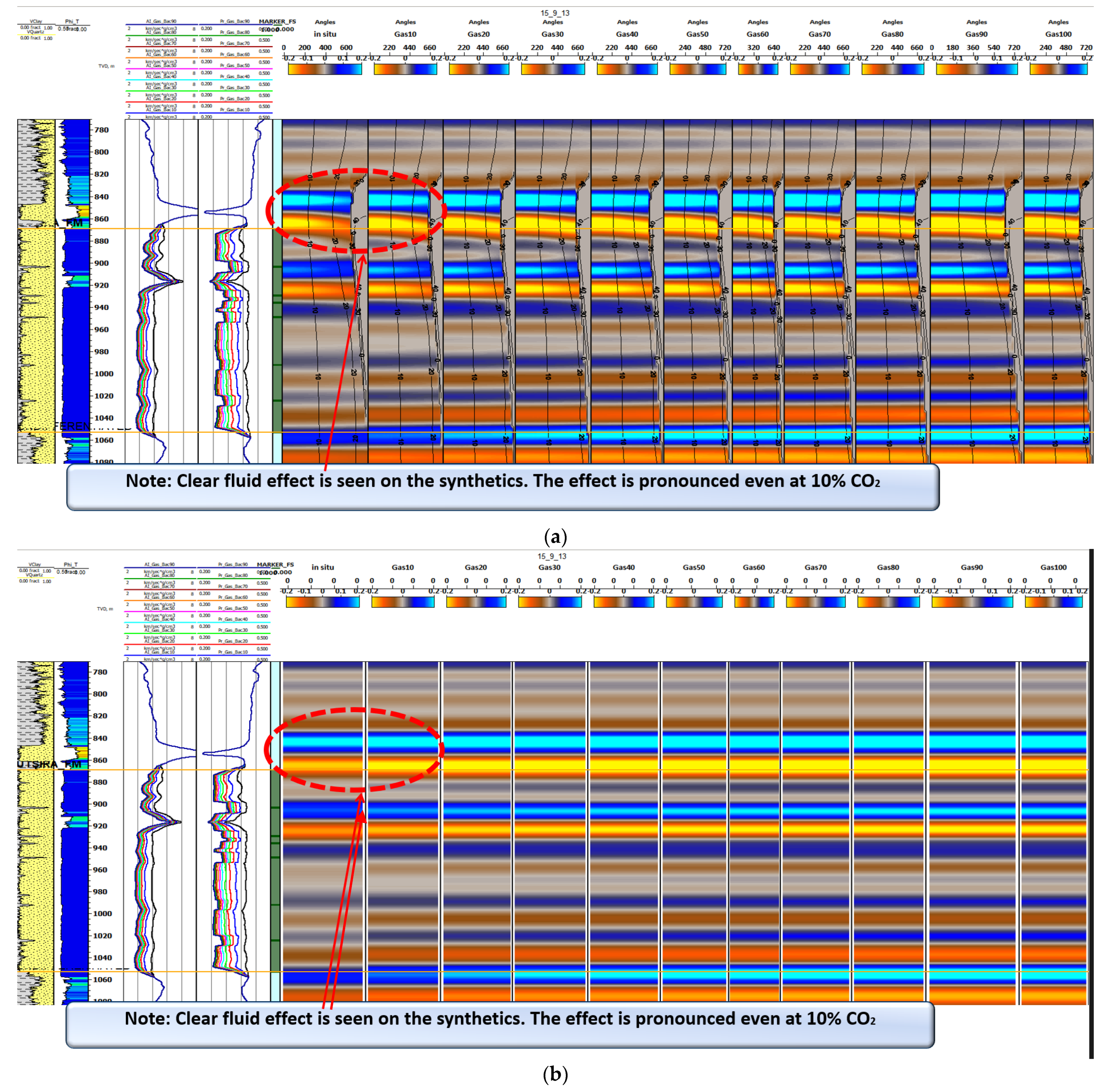
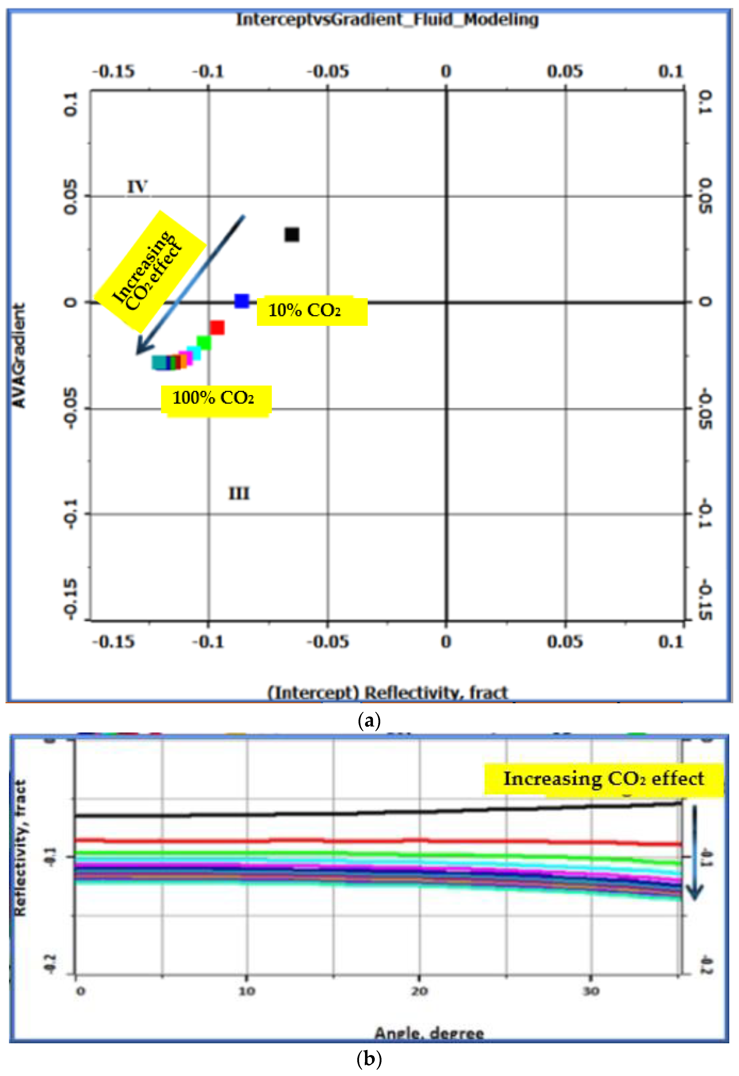
3.1.5. CO2 Fluid Substitution

CO2 fluid substitution is performed in the Utsira Formation in well 15/9-F1A, and different stages of CO2 injection (0–100% CO2 saturation at every 10%) are modeled. This section’s missing elastic logs have been predicted using the established rock physics model and calibrated using nearby wells and wells from Sleipner fields. Full-offset synthetic seismograms are then generated for all fluid models using a ray-tracing method.
The fluid substitution models employed in this study were built using the calibrated rock physics model and Biot—Gassmann theories [30,44,45]. For the partial saturation in brine and supercritical CO2, an effective fluid phase with different average techniques, used as “one fluid phase” as an input into the Biot theory for saturated porous media, is used [46,47]. In this instance, the microscopic description of the porous medium consists of a set of properties for each solid and fluid phase.
The equation of state is used to determine the fluid phase characteristics of brine and CO2 in the Utsira Sands [48]. The reservoir pressure and temperature conditions, which range from 8 to 11 MPa and 27 °C and 37 °C, respectively, have a significant effect on the supercritical CO2 phase properties [49].

4. Results and Discussion

In this study, Volve field data (well-logs and seismic) have been investigated for petrophysical properties, and qualitative and quantitative methods were used to identify the hydrocarbon-bearing reservoirs. In all of the wells, the reservoir sands have an average thickness of about 40 ft. They are characterized by low bulk densities, low relative P-wave velocities, high resistivities, and high porosities, compared to the overlying shale. Figure 4 shows that the Hugin Formation has good quality reservoir properties, with an average porosity of 0.23 porosity units, a thickness of about 100 m, a net-to-gross ratio of 0.9, and hydrocarbon saturation of about 80%.

4.1. Impact of Rock Physics Diagnostics

The sand sediment models exhibited distinct characteristics in our study, with the stiff sand sediment model proving to be the most suitable for representing our sands, while the soft sediment model emerged as the optimal choice for characterizing the sediments within the shales lithologies. In Figure 5, we have color-coded the measured data in black, and the final edited data are represented by clay volume.
The model lines presented in the figure delineate the trends in rock physics predicated on a single mineral solid framework. Specifically, the brown line corresponds to the stiff sediment model, consisting of 100% quartz, while the red line signifies the soft sediment model, comprising 100% clay. It is noteworthy that the data points enclosed in amber-colored ellipse denote bad data points, which have undergone correction through the application of our calibrated rock physics models.

4.2. Rock Physics Modeling

The various modeling scenarios were perturbed using Gassmann’s fluid substitution method. Utilizing rock physics analyses from the well data, we successfully identified the reservoirs and distinguished between various fluid and lithology effects within the study area. This information is succinctly presented in Figure 6a, which showcases a log display summarizing the outcomes of the fluid and synthetic modeling at in situ reservoir conditions. Notably, the AVA Pick domain, highlighted in magenta, represents the location of the AVA (amplitude versus angle) analysis.
The observations from Figure 6a reveal that the hydrocarbon-bearing sands exhibit lower Vp/Vs (compressional wave velocity to shear wave velocity ratio) and P-wave impedance (AI) values compared to the water-saturated sands. Additionally, the synthetic modeling results indicate that, at around 2.42 s, the in situ and hydrocarbon scenarios exhibit brighter amplitude responses than the wet scenario; moreover, there is a significant difference in the amplitude between the wet Vs hydrocarbon synthetic seismograms, with the difference reaching as high as 10%. The AVA analyses conducted at approximately 2.42 s further substantiate these findings, as follows: the hydrocarbon and in situ scenarios display a class III AVA response, characterized by an AVA gradient of approximately −0.025 and a reflectivity of around −0.04, while the wet scenario demonstrates a class IV AVA response, with an AVA gradient of about 0.01.
In Figure 6b, which depicts the cross plot results of the in situ conditions, we can observe a clear separation in the Vp/Vs and P-impedance domains, allowing for the differentiation of lithology and fluid effects. The distinction between the reservoir and the background trend is notably well defined. Furthermore, there is a marked sensitivity to fluid variations among the different scenarios, enabling the discrimination of hydrocarbon-rich conditions from water-saturated ones.
The favorable combination of substantial porosities and thickness in the Hugin Formation window sands makes them highly suitable for distinguishing between lithology and fluid properties under in situ rock property conditions.

Lithology Modeling

The results from the clay volume and porosity perturbation modeling (Figure 7, Figure 8 and Figure 9) illustrate how the elastic properties changed as the porosity, clay volume, and fluid changed. With increasing Vclay and reducing porosities, although the sensitivity is lowered, the sands are still suitable for lithology/fluid discrimination, due to their good thickness (Figure 7, Figure 8 and Figure 9). Figure 7 shows the modeling results of reducing the porosities by 10 porosity units, and we see that good separation from the background trend is still observed. Although the fluid sensitivity is reduced, but there is still a relatively fair separation between the fluid scenarios and in the AVA domain, the wet scenario shows a class IIP response, while the hydrocarbon scenario shows a class II response. Overall, the sands’ good thickness makes them relatively suitable for lithofluid discrimination, even at reduced porosity (although the sensitivity is reduced).
Figure 8 shows the cross plots depicting the modeling results when the reservoir condition is made shalier by increasing the clay volume by 20%. Here, what we see is that, even at the shalier reservoir condition, there is still a reasonable separation between the reservoir sands and the background; furthermore, there is a good discrimination between the wet and hydrocarbon scenario, especially in the upscaled domain. The sands’ good thickness makes them relatively suitable for lithofluid discrimination, even at a reduced clay content (although the sensitivity is reduced when compared to the in situ reservoir condition).
Figure 9 shows the result of increasing the clay content by 20% and reducing the porosity by 0.1 porosity unit, which is the worst reservoir scenario expected in this field. The sands are still fairly separable from the background trend in the Vp/Vs ratio and P-impedance domain, although separating our wet reservoirs and hydrocarbon sands might be a bit challenging in this domain. In the AVA domain, the wet sands show a class IV AVA response, while the hydrocarbon scenario shows a class II AVA response.

4.3. Seismic Inversion and Petrophysical Property Prediction

Figure 10 shows the inverted primary wave impedance (AI), shear wave impedance (SI), and the density for the seismic section inline 10,154. The inversion analysis shows a good fit between the inverted logs and the original logs (Figure 11). The simultaneous and sequential prediction results are shown in Figure 12, Figure 13 and Figure 14.
The inversion was then carried out after effectively tweaking the impedance parameters with the help of the cross plots from the well information [50,51]. The time slices taken at 2400 ms, with a window centered on the target and a fixed size of 10 ms, highlight the simultaneous and sequential prediction results. The black broken lines show the reservoir bounds. The previously known reservoir area around one of the wells has a low shale volume, high porosity, and low water saturation, which correlates well with our results (Figure 12, Figure 13 and Figure 14).
There is a strong correlation (or dependence) between lithology and porosity, therefore, predicting Vclay first and subsequently using Vclay as an input for porosity prediction improved our results. Overall, our results show that the sequential prediction approach produces a higher accuracy result (with the RMS error between the predicted and the original data being 0.31) than the simultaneous algorithm (with an RMS error of 0.45).

4.4. CO2 Modeling Results

Figure 15 shows a log plot of well 15/9-F1A, highlighting the Utsira Formation. After applying fluid substitution to the Utsira Formation and generating synthetic seismic traces for each CO2 saturation state, a clear fluid effect can be seen.
There is a sharp decrease in Vp (fizz-gas effect) when CO2 is introduced into a porous medium, whereas the change in velocity is minimal when the CO2 saturation is greater than 20%. Figure 16, Figure 17 and Figure 18 summarize the modeling results. Between 0 and 0.1 CO2 saturation, there is a dramatic decrease in the P-wave velocities (Figure 16a), with a subtle difference observed for higher saturation. With increasing CO2 saturation, the rock bulk modulus (Ksat) decreases. Consequently, the P-wave velocity decreases when the bulk density (b) decreases. At a CO2 saturation of 0.1%, the P-wave velocity increases subtly, due to a decrease in density.
In contrast, the increase in S-wave velocity is directly related to CO2 saturation (Figure 16b). Since the shear modulus remains constant and is unaffected by fluid substitution, the change in S-wave velocity depends only on the bulk density variations.
Figure 17 and Figure 18 summarize our modeling results, while Figure 19a,b show the synthetic seismogram and stack results. The distinction in the synthetic traces is most noticeable in the fluid substitution zone (~881–1070 m). With the CO2 increment, the amplitude values in the top reflector (881 m) change due to the substitution. The P-wave impedance reduction is visible and highlighted at 881 m. A huge reduction occurs between 0 and 10% CO2 saturation, with only minor variations observed at higher saturation levels. The AVO results (Figure 20) at 881 m show a strong effect from 0 to 0.1 CO2 saturation, with a sharp drop in the AVA gradient (−0.06 to −0.08) and intercept (0.03 to 0).

5. Conclusions

The results of the petrophysical inversion show that the sequential prediction approach produces a higher resolution than the simultaneous case in this Volve example. Because of their high porosities and thicknesses, the sands in the Hugin Formation window are suitable for lithofluid discrimination, according to the Vclay/porosity modeling results. The impact is particularly noticeable in the in situ conditions for most of the wells in the upscaled domain. Overall, the outcomes in every Volve field well are consistent. However, separating the hydrocarbon scenarios (oil vs. gas) could be difficult. The cross plots of AI vs. PR colored with facies also demonstrate the effectiveness of discrimination in this area.
Due to the good accuracy in the inversions and log analysis, we undertook fluid substitution studies for possible CO2 sequestration. The modeling of the CO2 fluids helped us to model the conditions in the area of interest and the seismic changes that occurred throughout the various stages of CO2 injection (0% to 100% CO2 saturation). The following could be observed in the first 10% CO2 substitution: The typical decrease in P-wave velocity is 12%. The Vs increases in direct proportion to CO2 saturation. A subtle effect is observed for higher CO2 saturation values. The decrease in Vp and density represents a decrease in the impedance and reflectivity contrast.

Author Contributions

Conceptualization, D.P.-D. and R.R.S.; methodology, D.P.-D.; software, D.P.-D.; validation, R.R.S.; formal analysis, D.P.-D.; investigation, R.R.S.; resources, D.P.-D. and R.R.S.; data curation, D.P.-D.; writing—original draft preparation, D.P.-D.; writing—review and editing, D.P.-D. and R.R.S.; visualization, D.P.-D. and R.R.S.; supervision, R.R.S.; project administration, D.P.-D. and R.R.S.; and funding acquisition, R.R.S. All authors have read and agreed to the published version of the manuscript.

Funding

This research was funded by Subsea Systems Institute and Allied Geophysics Laboratory (AGL) at the University of Houston.

Institutional Review Board Statement

Not applicable.

Informed Consent Statement

Not applicable.

Data Availability Statement

Data is available upon request from the authors.

Acknowledgments

The authors would like to thank Ayodeji Babalola, Robert Keirstead and William Marin for their technical support. We also wish to express our gratitude to Equinor for providing the data, PGS and CGG for providing the software, and the Allied Geophysics Laboratory (AGL) at the University of Houston for their support.

Conflicts of Interest

The authors declare no conflicts of interest.

Appendix A

Keras, a high-level neural network API, was applied. The sequential model in Keras simplifies the process of model building into the stacking of layers. Each layer in the sequential model is a transformation function that accepts a weighted input and produces an output through an activation function. For continuous variable predictions, architectures with multiple hidden layers, known as deep networks, are common. Within the scope of this research, a sequential model with 20 hidden layers, each employing the sigmoid activation function, was utilized to approximate non-linear mapping between the input features and a continuous target variable. The mathematical summary of how a sequential model works in the context of a feedforward neural network is summarized in Equation (A1).
Keras models require compilation before training, where the choice of the loss function and the optimizer is specified. Given the continuous nature of the target variable, the mean squared error (MSE) was employed as the loss function. For optimization, the Adam optimizer was selected for its adaptive learning rate capabilities, which adjust as per the learning gradient of each weight, leading to faster convergence. A sequential model is composed of n layers, where each layer l has a function f l that transforms its input x l 1 into an output x ( l ) , which then becomes the input to the next layer. The training process involves the forward propagation of the input data through the network and the backpropagation of the errors to update the model weights. In the implementation, Keras handles the intricacies of the backpropagation, while the Adam optimizer adjusts the weights in a manner that minimizes the loss function. The optimization algorithm’s hyperparameters, such as the learning rate and the first and second moment decay rates, were tuned to enhance the model’s predictive performance.
The general mathematical representation of the transformation at each layer l is as follows:
x ( l ) = f l ( W l · x l 1 + b l )
where:
  • W l represents the weights matrix for layer l.
  • b ( l ) represents the bias vector for layer l.
  • f l represents the activation function for layer l.
For further technical details and mathematical formulations, you can refer to [52,53]. Also, the source of data used in this study can be found in [54,55].

References

  1. Anees, M. Seismic Attribute Analysis for Reservoir Characterization. In Proceedings of the 10th Biennial International Conference and Exposition, Kochi, India, 23–25 November 2013. [Google Scholar]
  2. Guo, Q.; Ba, J.; Fu, L.-Y.; Luo, C. Joint seismic and Petrophysical nonlinear inversion with gaussian mixture-based adaptive regularization. Geophysics 2021, 86, 895–911. [Google Scholar] [CrossRef]
  3. González, E.F.; Mukerji, T.; Mavko, G. Seismic inversion combining rock physics and multiple-point geostatistics. Geophysics 2008, 73, R11–R21. [Google Scholar] [CrossRef]
  4. Sen, M.K.; Stoffa, P.L. Global Optimization Methods in Geophysical Inversion; Cambridge University Press: Cambridge, UK, 2013. [Google Scholar]
  5. Dvorkin, J.; Grana, D.; Gutierrez, M.A. Seismic Reflections of Rock Properties; Cambridge University Press: Cambridge, UK, 2014. [Google Scholar]
  6. Schuster, G.T. Seismic Inversion; Society of Exploration Geophysicists: Houston, TX, USA, 2017; Volume 20. [Google Scholar] [CrossRef]
  7. Sokolov, A.; Schulte, B.; Shalaby, H.; Molen, M. Seismic inversion for reservoir characterization. In Applied Techniques to Integrated Oil and Gas Reservoir Characterization; Elsevier: Amsterdam, The Netherlands, 2021; pp. 329–351. [Google Scholar] [CrossRef]
  8. Amaro, C.; Grana, D.; Azevedo, L.; Soares, A. Geostatistical Seismic Inversion Integrating Rock Physics Models. In Proceedings of the 78th EAGE Conference and Exhibition 2016, Vienna, Austria, 30 May–2 June 2016. [Google Scholar] [CrossRef]
  9. Chopra, S.; Marfurt, K.J. Seismic Attributes for Prospect Identification and Reservoir Characterization; Society for Exploration Geophysicists: Houston, TX, USA, 2007; Volume 2, pp. 1–16. [Google Scholar] [CrossRef]
  10. Garia, S.; Pal, A.K.; Ravi, K.; Nair, A.M. Prediction of petrophysical properties from seismic inversion and Neural Network: A case study. In Proceedings of the EGU General Assembly Conference 2021, Online, 19–20 April 2021; p. EGU21-11824. Available online: https://ui.adsabs.harvard.edu/link_gateway/2021EGUGA..2311824G/doi:10.5194/egusphere-egu21-11824 (accessed on 1 January 2024).
  11. Ruiz, R.; Roubickova, A.; Reiser, C.; Banglawala, N. Data Mining and machine learning for porosity, saturation, and shear velocity prediction: Recent experience and results. First Break 2021, 39, 71–76. [Google Scholar] [CrossRef]
  12. Bressan, T.S.; de Souza, M.K.; Girelli, T.J.; Junior, F.C. Evaluation of machine learning methods for lithology classification using geophysical data. Comput. Geosci. 2020, 139, 104475. [Google Scholar] [CrossRef]
  13. Hou, M.; Xiao, Y.; Lei, Z.; Yang, Z.; Lou, Y.; Liu, Y. Machine Learning Algorithms for Lithofacies Classification of the Gulong Shale from the Songliao Basin, China. Energies 2023, 16, 2581. [Google Scholar] [CrossRef]
  14. Yang, L.; Sun, S.Z. Seismic horizon tracking using a deep convolutional neural network. J. Pet. Sci. Eng. 2020, 187, 106709. [Google Scholar] [CrossRef]
  15. Ismail, A.; Radwan, A.A.; Leila, M.; Abdelmaksoud, A.; Ali, M. Unsupervised machine learning and multi-seismic attributes for fault and fracture network interpretation in the Kerry Field, Taranaki Basin, New Zealand. Geomech. Geophys. Geo-Energy Geo-Resour. 2023, 9, 122. [Google Scholar] [CrossRef]
  16. Di, H.; Li, Z.; Maniar, H.; Abubakar, A. Seismic stratigraphy interpretation by deep convolutional neural networks: A semisupervised workflow. Geophysics 2020, 85, 77–86. [Google Scholar] [CrossRef]
  17. Tensorflow. Module: TF: Tensorflow Core v2.8.0. TensorFlow. 2021. Available online: https://www.tensorflow.org/api_docs/python/tf (accessed on 20 December 2021).
  18. Kappler, K.; Kuzma, H.A.; Rector, J.W. A comparison of standard inversion, neural networks and support Vector Machines. SEG Tech. Program Expand. Abstr. 2005, 2005, 1725–1727. [Google Scholar] [CrossRef]
  19. Kim, Y.; Nakata, N. Geophysical inversion versus machine learning in inverse problems. Lead. Edge 2018, 37, 894–901. [Google Scholar] [CrossRef]
  20. Oyetunji, O.; Stewart, R. Reservoir characterization using petrophysical analysis of the Volve Field, Norway. In Proceedings of the EAGE Annual 82nd Conference & Exhibition 2021, Amsterdam, The Netherlands, 28–30 October 2021. [Google Scholar] [CrossRef]
  21. Ravasi, M.; Vasconcelos, I.; Curtis, A.; Kritski, A. Vector-acoustic reverse time migration of Volve ocean-bottom cable data set without up/down decomposed wavefields. Geophysics 2015, 80, S137–S150. [Google Scholar] [CrossRef]
  22. Norwegian Petroleum Directorate. 4.1—Geology of the North Sea—The Norwegian Petroleum Directorate. Available online: https://www.npd.no/en/whats-new/publications/co2-atlases/co2-atlas-for-the-norwegian-continental-shelf/4-the-norwegian-north-sea/4.1-geology-of-the-north-sea/ (accessed on 1 January 2024).
  23. Wang, B.; Sharma, J.; Chen, J.; Persaud, P. Ensemble machine learning assisted reservoir characterization using field production data–an offshore field case study. Energies 2021, 14, 1052. [Google Scholar] [CrossRef]
  24. Jackson, C.A.-L.; Kane, K.E.; Larsen, E. Structural evolution of minibasins on the utsira high, northern North Sea; implications for Jurassic sediment dispersal and reservoir distribution. Pet. Geosci. 2010, 16, 105–120. [Google Scholar] [CrossRef]
  25. Zweigel, P.; Arts, R.; Lothe, A.E.; Lindeberg, E.B. Reservoir geology of the Utsira Formation at the first industrial-scale underground co 2 storage site (Sleipner area, North Sea). Geol. Soc. Lond. Spec. Publ. 2004, 233, 165–180. [Google Scholar] [CrossRef]
  26. Al Ghaithi, A.; Prasad, M. Machine learning with artificial neural networks for shear log predictions in the Volve Field Norwegian North Sea. In SEG Technical Program Expanded Abstracts; Society of Exploration Geophysicists: Houston, TX, USA, 2020; pp. 450–454. [Google Scholar] [CrossRef]
  27. Arts, R.; Eiken, O.; Chadwick, A.; Zweigel, P.; van der Meer, L.; Zinszner, B. Monitoring of CO2 injected at Sleipner using time-lapse seismic data. Energy 2004, 29, 1383–1392. [Google Scholar] [CrossRef]
  28. Equinor. Volve Field Data Set Download. Volve Field Data Village Download—Data 2008–2016. 2020. Available online: https://www.equinor.com/en/what-we-do/digitalisation-in-our-dna/volve-field-data-village-download.html (accessed on 12 December 2020).
  29. Mukerji, T.; Dutta, N.; Prasad, M.; Dvorkin, J. Seismic Detection and Estimation of Overpressures Part I: The Rock Physics Basis. CSEG Rec. 2002, 27, 34–57. [Google Scholar]
  30. Gassmann, F. On the elasticity of porous media: Quarterly publication of the Natural Research Society in Zurich. Geophysics 1951, 96, 1–23. [Google Scholar]
  31. Adam, L.; Batzle, M.; Brevik, I. Gassmann’s fluid substitution and shear modulus variability in carbonates at laboratory seismic and ultrasonic frequencies. Geophysics 2006, 71, F173–F183. [Google Scholar] [CrossRef]
  32. Greenberg, M.L.; Castagna, J.P. Shear-wave velocity estimation in porous rocks: Theoretical formulation, preliminary verification and applications. Geophys. Prospect. 1992, 40, 195–209. [Google Scholar] [CrossRef]
  33. Mavko, G.; Mukerji, T.; Dvorkin, J. The Rock Physics Handbook; Cambridge University Press: Cambridge, UK, 2020. [Google Scholar]
  34. de Figueiredo, L.P.; Grana, D.; Santos, M.; Figueiredo, W.; Roisenberg, M.; Schwedersky Neto, G. Bayesian seismic inversion based on rock-physics prior modeling for the joint estimation of acoustic impedance, porosity and lithofacies. J. Comput. Phys. 2017, 336, 128–142. [Google Scholar] [CrossRef]
  35. Smith, T.M.; Sondergeld, C.H.; Rai, C.S. Gassmann fluid substitutions: A tutorial. Geophysics 2003, 68, 430–440. [Google Scholar] [CrossRef]
  36. Batzle, M.; Wang, Z. Seismic properties of pore fluids. Geophysics 1992, 57, 1396–1408. [Google Scholar] [CrossRef]
  37. Buland, A.; El Ouair, Y. Bayesian time-lapse inversion. Geophysics 2006, 71, R43–R48. [Google Scholar] [CrossRef]
  38. Aki, K.; Richards, P.G. Quantitative seismology, theory and methods. J. Acoust. Soc. Am. 1980, 68, 1546. [Google Scholar] [CrossRef]
  39. Stolt, R.H.; Weglein, A.B. Migration and inversion of Seismic Data. Geophysics 1985, 50, 2458–2472. [Google Scholar] [CrossRef]
  40. Hampson, D.P.; Russell, B.H.; Bankhead, B. Simultaneous inversion of pre-stack seismic data. SEG Tech. Program Expand. Abstr. 2005, 7, 1633–1637. [Google Scholar] [CrossRef]
  41. Gardner, G.H.; Gardner, L.W.; Gregory, A.R. Formation velocity and density—The diagnostic basics for stratigraphic traps. Geophysics 1974, 39, 770–780. [Google Scholar] [CrossRef]
  42. Dramsch, J.S. 70 years of machine learning in Geoscience in review. Mach. Learn. Geosci. 2020, 61, 1–55. [Google Scholar] [CrossRef]
  43. Kingma, D.P.; Ba, J. Adam: A Method for Stochastic Optimization. arXiv 2015, arXiv:1412.6980. [Google Scholar]
  44. Biot, M.A. Theory of propagation of elastic waves in a fluid-saturated porous solid. I. Low-Frequency Range. J. Acoust. Soc. Am. 1956, 28, 168–178. [Google Scholar] [CrossRef]
  45. Pelemo-Daniels, D.; Nwafor, B.O.; Stewart, R.R. CO2 Injection Monitoring: Enhancing Time-Lapse Inversion for Injected Volume Estimation in the Utsira Formation, Sleipner Field, North Sea. J. Mar. Sci. Eng. 2023, 11, 2275. [Google Scholar] [CrossRef]
  46. Pride, S.R.; Berryman, J.G.; Harris, J.M. Seismic attenuation due to wave-induced flow. J. Geophys. Res. Solid Earth 2004, 109, 1–19. [Google Scholar] [CrossRef]
  47. Müller, T.M.; Gurevich, B.; Lebedev, M. Seismic wave attenuation and dispersion resulting from wave-induced flow in porous rocks—A review. Geophysics 2010, 75, 147–164. [Google Scholar] [CrossRef]
  48. Span, R.; Wagner, W. A new equation of state for carbon dioxide covering the fluid region from the triple-point temperature to 1100 K at pressures up to 800 MPA. J. Phys. Chem. Ref. Data 1996, 25, 1509–1596. [Google Scholar] [CrossRef]
  49. Ghaderi, A.; Landrø, M. Estimation of thickness and velocity changes of injected carbon dioxide layers from prestack time-lapse seismic data. Geophysics 2009, 74, 17–28. [Google Scholar] [CrossRef]
  50. Nwafor, B.O.; Hermana, M.; Elsaadany, M. Geostatistical Inversion of Spectrally Broadened Seismic Data for Re-Evaluation of Oil Reservoir Continuity in Inas Field, Offshore Malay Basin. J. Mar. Sci. Eng. 2022, 10, 727. [Google Scholar] [CrossRef]
  51. Nwafor, B.O.; Hermana, M. Harmonic Extrapolation of Seismic Reflectivity Spectrum for Resolution Enhancement: An Insight from Inas Field, Offshore Malay Basin. Appl. Sci. 2022, 12, 5453. [Google Scholar] [CrossRef]
  52. Chollet, F. Deep Learning with Python; Manning Publications: Shelter Island, NY, USA, 2017. [Google Scholar]
  53. Goodfellow, I.; Bengio, Y.; Courville, A. Deep Learning; The MIT Press: Cambridge, MA, USA, 2017. [Google Scholar]
  54. Equinor. Sleipner 4D Seismic Dataset. 2020. Available online: https://co2datashare.org/dataset/sleipner-4d-seismic-dataset (accessed on 1 January 2024).
  55. Equinor. Volve Field Dataset; Volve Field Data Set Download—Equinor. 2020. Available online: https://www.equinor.com/energy/volve-data-sharing (accessed on 1 January 2024).
Figure 1. Map showing the Volve and Sleipner fields, Norwegian North Sea [21].
Applsci 14 01345 g001
Figure 3. Petrophysical inversion workflow.
Applsci 14 01345 g003
Figure 4. Well logs showing one of the identified reservoir zones. From the left: Caliper, GR, deep resistivity, clay volume, porosity, saturation, depth tracks, density, Vp, Vs, AI, Vp/Vs, and Poisson’s ratio (PR). The rock physics model curves are shown in blue, the original logs are shown in red, and the final edited curves are shown in black.
Applsci 14 01345 g004
Figure 5. Vp versus density cross plot color-coded by Vclay (fraction). The model lines depict trends in rock physics based on a single mineral solid frame. The brown line represents the stiff sediment model, which is 100% quartz, while the red line represents the soft sediment model, which is 100% clay. The soft sediment model best represents all high clay lithologies, while the stiff sediment model covers the quartz lithologies. The highlighted data enclosed in yellow circle are the bad data that have been corrected using the rock physics models.
Applsci 14 01345 g005
Figure 6. (a) Log plot showing the modeling results (in situ scenario). (b) Cross plots showing the modeling results (in situ scenario). Hydrocarbon sands displayed lower Vp/Vs and P-wave impedance (AI) values than wet sands. Strong ability to discriminate fluids, particularly in the AVA domain.
Applsci 14 01345 g006aApplsci 14 01345 g006b
Figure 7. Cross plots showing the modeling results (negative 10 p.u. scenario). The sands’ good thickness makes them relatively suitable for lithofluid discrimination, even at reduced porosity (although the sensitivity is reduced).
Applsci 14 01345 g007
Figure 8. Cross plots showing the modeling results (positive Vclay 0.2 scenario). The sands’ good thickness makes them relatively suitable for lithofluid discrimination, even at reduced porosity (although the sensitivity is reduced).
Applsci 14 01345 g008
Figure 9. Cross plots showing the modeling results (PosVclay 0.2, Neg Por10 p.u. scenario). The sands’ good thickness makes them relatively suitable for lithofluid discrimination, even at reduced porosity (although the sensitivity is reduced).
Applsci 14 01345 g009
Figure 10. Inverted seismic section showing (from top to bottom) the P-wave impedance, S-wave impedance, and density for the seismic section (inline 10,154).
Applsci 14 01345 g010
Figure 11. Machine-learning prediction at well 15/9-18A.
Applsci 14 01345 g011
Figure 12. Time slices of the shale volume inversion taken at 2400 ms—From the left, sequential and simultaneous approaches, respectively.
Applsci 14 01345 g012
Figure 13. Time slices of the porosity inversion taken at 2400 ms—From the left, sequential and simultaneous approaches, respectively.
Applsci 14 01345 g013
Figure 14. Time slices of the water saturation inversion taken at 2400 ms—From the left, sequential and simultaneous approaches, respectively.
Applsci 14 01345 g014
Figure 15. Petrophysical analyses—Zone of Interest (ZoI).
Applsci 14 01345 g015
Figure 16. (a) P-wave velocity change versus CO2 saturation. An abrupt drop in P-wave velocity values, especially between 0 and 0.2 CO2 saturation, and (b) S-wave velocity change versus CO2 saturation. CO2 saturation has a direct relationship with S-wave velocity.
Applsci 14 01345 g016
Figure 17. Cross plot of AI versus PR color-coded by Vclay. The arrow illustrates the decreasing CO2 effect, showing a sharp effect from 0 to 0.2 CO2 saturation, while a more subtle effect is observed for higher CO2 saturation values.
Applsci 14 01345 g017
Figure 18. Fluid modeling results from left to right: lithology, porosity, saturation, depth density, Vp, Vs, AI, and PR tracks. The arrow shows the decreasing CO2 effect.
Applsci 14 01345 g018
Figure 19. (a) Fluid modeling synthetic gathers. From left to right, there is an increasing CO2 effect. As highlighted in red, the most significant drop occurs between 0 and 10% CO2 saturation, with only minor variations observed at higher saturation levels. (b) fluid modeling synthetic stacks. From left to right, there is an increasing CO2 effect. As highlighted in red, the most significant drop occurs between 0 and 10% CO2 saturation, with only minor variations observed at higher saturation levels.
Applsci 14 01345 g019
Figure 20. (a) Cross plot of intercept vs. AVA gradient fluid modeling results. AVO results show a strong effect from 0 to 0.1 CO2 saturation, with a sharp drop in AVA gradient (−0.06 to −0.08) and intercept (0.03 to 0). A subtle effect is observed for higher CO2 saturation values. (b) Cross plot of angle vs. reflectivity, where sharp drop in reflectivity is observed from 0 to 0.1 CO2 saturation. A subtle effect is observed for higher CO2 saturation values.
Applsci 14 01345 g020
Disclaimer/Publisher’s Note: The statements, opinions and data contained in all publications are solely those of the individual author(s) and contributor(s) and not of MDPI and/or the editor(s). MDPI and/or the editor(s) disclaim responsibility for any injury to people or property resulting from any ideas, methods, instructions or products referred to in the content.

