Article

Brain Extraction Methods in Neonatal Brain MRI and Their Effects on Intracranial Volumes

1
Instituto de Biofísica e Engenharia Biomédica, Faculdade de Ciências da Universidade de Lisboa, 1749-016 Lisbon, Portugal
2
Department of Neuroradiology, Karolinska University Hospital, SE-171 76 Stockholm, Sweden
3
Department of Women’s and Children’s Health, Uppsala University, SE-751 85 Uppsala, Sweden
*
Author to whom correspondence should be addressed.
Appl. Sci. 2024, 14(4), 1339; https://doi.org/10.3390/app14041339
Submission received: 31 December 2023 / Revised: 29 January 2024 / Accepted: 2 February 2024 / Published: 6 February 2024
(This article belongs to the Special Issue Methods, Applications and Developments in Biomedical Informatics)

Abstract

:
Magnetic resonance imaging (MRI) plays an important role in assessing early brain development and injury in neonates. When using an automated volumetric analysis, brain tissue segmentation is necessary, preceded by brain extraction (BE) to remove non-brain tissue. BE remains challenging in neonatal brain MRI, and despite the existence of several methods, manual segmentation is still considered the gold standard. Therefore, the purpose of this study was to assess different BE methods in the MRI of preterm neonates and their effects on the estimation of intracranial volumes (ICVs). This study included twenty-two premature neonates (mean gestational age ± standard deviation: 28.4 ± 2.1 weeks) with MRI brain scans acquired at term, without detectable lesions or congenital conditions. Manual segmentation was performed for T2-weighted scans to establish reference brain masks. Four automated BE methods were used: Brain Extraction Tool (BET2); Simple Watershed Scalping (SWS); HD Brain Extraction Tool (HD-BET); and SynthStrip. Regarding segmentation metrics, HD-BET outperformed the other methods with median improvements of +0.031 (BET2), +0.002 (SWS), and +0.011 (SynthStrip) points for the dice coefficient; and −0.786 (BET2), −0.055 (SWS), and −0.124 (SynthStrip) mm for the mean surface distance. Regarding ICVs, SWS and HD-BET provided acceptable levels of agreement with manual segmentation, with mean differences of −1.42% and 2.59%, respectively.

1. Introduction

Magnetic resonance imaging (MRI) plays an important role in assessing early brain development and injury in neonates through clinical interpretation and volumetric analyses (e.g., intracranial volume (ICV) and regional brain volume measurements) [1,2]. In this context, image acquisition and assessment pose unique challenges [2,3,4]: (1) fast imaging sequences, with the incomplete filling of the k-space, are typically used in order to avoid sedation and movement artifacts, but at the expense of image quality; (2) the use of two-dimensional (2D) sequences with thick slices to further decrease the acquisition time leads to partial volume effects which may compromise the assessment of the small brain structures being imaged; (3) the contrast-to-noise ratio (CNR) between grey and white matter may be lower if imaging sequences are not optimized regarding repetition and echo times; (4) if dedicated coils are not available, the signal-to-noise ratio (SNR) might also be compromised; (5) the appearance of the brain and regional structures differs from the adult brain and undergoes rapid changes with gestational age (GA) and postnatal maturation (due to evolving myelination, decreases in brain water content, and an increase in tissue density); (6) abnormalities may be related to specific perinatal pathologies that are not typically observed in adults and usually evolve rapidly; and (7) image processing methods also vary across premature newborns, infants, and adults.
As an essential pre-processing step for brain tissue segmentation and image registration, brain extraction (BE) or skull stripping is necessary to remove non-brain tissue [5,6,7]. This is a critical step because inaccurate intracranial segmentation, e.g., unremoved non-brain tissues or incorrectly removed brain tissues, could result in the under- or over-estimation of brain volumes [5].
There are several methods for BE (i.e., manual, semi-automated, and automated algorithms), but manual segmentation is still considered the gold standard or ground truth for BE; despite being time consuming and having inter/intra-rater variability, they are often used to validate semi-automatic and automatic methods [6,7,8,9,10,11]. These methods can be classified as follows: conventional methods (deformable surface-based, mathematical morphology, intensity, template, and hybrid-based models) as well as machine learning and deep learning methods [7,9,11]. The majority of the available methods are focused on the adult brain (e.g., BEaST [12], BEMA [13], BET [8], BET2 [14], BSE [15], CONSNet [16], DMBE [17], FSW [18], HD-BET [19], MASS [20], McStrip [21], ROBEX [22], MONSTR [23], SBA [24], SPECTRE [25], SynthStrip [26], 3dSkullStrip [27], and the 3D U-Net approach [28]), but some have been optimized or developed specifically for neonates (e.g., ALFA [29], iBEAT2 [30], LABEL [31], STAPLE [32], GCSP [10], HSS [33], AFSS [34], and the fuzzy object model-based fuzzy connectedness approach [35]).
BE remains challenging in neonatal brain MRI because of the low spatial resolution, low signal-to-noise ratio, low contrast-to-noise ratio, wide variation in intensity within tissues, small brain size, evolving shape, and motion artifacts when compared with adult brain images [5,6,11]. Additionally, most BE methods are designed to work with T1-weighted (T1w) MRI, but in neonates, these images lack contrast between brain tissues, so T2-weighted (T2w) images are most often used [1,2,36].
Therefore, the purpose of this study was to apply different BE methods in the MRI of preterm neonates and assess their performances, focusing on comparisons with manual segmentation as well as on the effect they have in estimating ICVs.

2. Materials and Methods

2.1. Subjects

The dataset used in this study consisted of pseudonymized MRI brain scans from 22 premature neonates (Table 1) without detectable brain lesions or congenital conditions, who had no severe motion artifacts and were scanned at term-equivalent age (TEA), which is considered the optimal timeframe for evaluating structural abnormalities that may have implications for long-term outcomes [37]. The MRI scans were performed as part of the clinical routine for very preterm infants at Uppsala University Hospital, a tertiary referral centre in Sweden, and parental consent was obtained for retrospective data analysis, as approved by the Human Research Ethical Committee of the Medical Faculty at Uppsala University (Dnr 2014/236).

2.2. MRI Protocol

All MRI scans were acquired on a Siemens Avanto 1.5 Tesla scanner (Siemens Medical Systems, Erlangen, Germany) at Uppsala University Hospital using a neonatal-adapted imaging protocol. To perform this study, 2D fast spin echo (FSE) T2w images were acquired with the following parameters: axial slice number = 33; slice thickness = 3 mm; gap distance factor 20% interleaved (spacing between slices = 3.6 mm); field-of-view (FOV) read/phase = 200 mm/100%; repetition time (TR) = 6520 ms; echo time (TE) = 103 ms; and flip angle = 120°.

2.3. Manual Segmentation for Brain Extraction

To create a reference brain mask for each image volume, a strictly defined, fully manual procedure was followed using the 3D Slicer (version 5.2.2) software [38]. The mask was drawn slice by slice in the axial plane, considering the cerebral contour [39], excluding non-brain structures, such as the neck, ears, eyes, scalp, and skull, with reference to brain atlases [40,41], using the original images without preprocessing as input. Each brain mask was also divided into stack of slices, creating three masks for each BE method, from the bottom to the top of the brain, to assess whether the methods produced different results depending on the anatomical region. The bottom mask—slices 1 to 11—covered the base of the skull, and part of brain stem and cerebellum (inferior limit: first slice, level of the spinal cord; superior limit: level of the pons, when the ocular globes and the lenses are visible). The middle mask—slices 12 to 22—included subcortical structures such as the basal ganglia (superior limit: below the level of the centrum semiovale). The top mask—slices 23 to 33—covered the centrum semiovale and the vertex (superior limit: top of the skull).
Rater 1 (T.F.V.) performed all segmentations, which were validated by another two experienced raters (rater 2—N.C.M. and rater 3—H.A.F.). To evaluate intra-rater reliability, rater 1 re-segmented six randomly chosen subjects from previously segmented data after one month. Inter-rater accuracy was assessed including segmentations from raters 2 and 3, which manually outlined six randomly selected subjects from the dataset.

2.4. Selection of Automated Brain Extraction Methods

The criteria for selection of the skull stripping methods were based on their public availability, citations, generalizability for a variety of contrasts, and use of state-of-the-art methods without published studies in neonates.
Four automated BE methods were used (Table 2): two conventional methods (Brain Extraction Tool (BET2) [14] and Simple Watershed Scalping (SWS) [42]) and two deep learning methods (HD Brain Extraction Tool (HD-BET) [19] and SynthStrip [26]). Again, each brain mask obtained for each method was also divided into stack of slices, following the same procedure as described in Section 2.3.
Finally, whereas the different BE methods can be used within toolboxes or as standalone programs, in this study, the respective toolboxes were used (second column of Table 2), with the exception of SynthStrip [26], which was used as a standalone program running in Docker [43] (the software versions can be found in Section 2.6).
Table 2. Selection of automated brain extraction methods.
Brain Extraction MethodSoftwareMethod Category [9]
Brain Extraction Tool (BET version 2.0, BET2) [8,14]FSL (FMRIB Software Library) [44]Deformable surface-based model
Simple Watershed Scalping (SWS)—unvalidated module in Morphologically Adaptive Neonate Tissue Segmentation (MANTiS, version 1.1) toolbox [42]SPM (Statistical Parametric Mapping) [45] running in MATLAB® [46] or as an open-source standaloneIntensity-based (watershed transform)
HD Brain Extraction Tool (HD-BET, version 1.0) [19]Extension of 3D Slicer [38] or as open-source standaloneDeep learning
(based on U-Net architecture and its 3D derivatives)
SynthStrip (version 1.3) [26]FreeSurfer [47] or as open-source standaloneDeep learning
(based on 3D U-Net)
BET2 [14] is based on BET [8], one of the most widely used methods for skull stripping, using the original model or several modified versions [6,7,9]. BET2 uses techniques such as intensity clamping, surface point detection, and mesh fitting to find the brain boundary in brain MRI [14]. Even though they do not have parameters optimized for neonates, they have been used in this context [42,48,49,50,51,52,53,54].
SWS is a preliminary version of a BE tool available within the Morphologically Adaptive Neonatal Tissue Segmentation (MANTiS) toolbox [42], based on watershed transform. It can be used before the tissue classification pipeline and has been used in several studies [55,56,57,58,59,60,61,62,63,64,65], although it was not used in the validation study of the toolbox (they used BET instead) as it was not available then.
HD-BET [19] relies on artificial neural networks and has outperformed six commonly used BE tools (BET [8], 3dSkullStrip [27], BSE [15], ROBEX [22], BEaST [12], and MONSTR [23]). The algorithm was trained with multi-sequence MRI from adults (precontrast T1w, postcontrast T1w, T2w, and fluid-attenuated inversion recovery (FLAIR)) with different MRI scanners and acquisition parameters and showed robustness even in the presence of pathology- or treatment-induced tissue alterations [19].
SynthStrip [26] builds on a solid foundation laid by prior studies of deep learning algorithms for BE, using a 3D U-Net convolutional architecture. It has generally produced highly accurate brain masks compared with other BE tools (BET [8], BEaST [12], DMBE [17], FSW [18], ROBEX [22], and 3dSkullStrip [27]). It is a flexible BE tool that can be deployed universally for a variety of brain images because it is agnostic to acquisition parameters, as it never samples any real data during training because a strategy for synthesizing diverse training data is applied. Its efficacy was demonstrated in a dataset, ranging from infants to adults, that included structural MRI (T1w, T2w, FLAIR, proton density weighted, MR angiography, computed tomography, and 18F-Fluorodeoxyglucose positron emission tomography.
HD-BET and SynthStrip are state-of-the-art BE methods reporting excellent results, andm to the best of our knowledge, there have not been focused research efforts on their BE performance in MRI preterm infants scanned at TEA.
From these methods, only BET2 and SynthStrip allowed for variations in options, and we systematically investigated their performance to identify the parameters that provided more accurate BE results compared with those of manual segmentation, since there are no references to use in neonates. Based on the results (Appendix A), we set these parameters to apply to the dataset.
As a note, we also tested the iBEAT2 BE method [30]. Nonetheless, at the time of this study, this method had some limitations: (1) it did not provide whole-brain parcellation, so when removing the brain skull, the cerebellum was also removed, and the final output could not be used to measure the ICV; and (2), when inserting the data details for the method, the minimum accepted age was 1 month (currently, the method accepts data from 0-month-old neonates that would be considered at the TEA). These limitations, therefore, precluded the use of this method and its comparison to others.

2.5. Measurement of Intracranial Volumes

ICV is defined as the volume inside the cranium [39,66], and in this study, the ICVs were estimated in mL with 3D Slicer (version 5.2.2) [38] from the intracranial masks obtained from each BE method (manual, BET2, SWS, HD-BET, and SynthStrip).

2.6. Hardware and Software

Our research was performed on a MacBook Pro Retina (Apple Inc., Cupertino, CA, USA) with a 2.7 GHz Intel Core i5 CPU and 8 GB of RAM. The manual segmentation was performed using an external 28” 4K UHD monitor (Lenovo L28u-35, Lenovo Group Ltd., Beijing, China) and a graphics tablet (GAOMON S620, Gaomon Technology Co., Guangzhou, China).
Several software were used to perform BE and volume measurements, such as the following: 3D Slicer (version 5.2.2) [38]; Docker (version 4.18.0) [43]; FSL (version 6.0.6.4) [44]; MATLAB® R2023a (version 9.14) [46]; and SPM12 (revision 7771) [45]. The segmentation metrics were computed in Python (version 3.11.2) [67], and all statistical analyses were performed with the IBM® SPSS® v27 software [68].

2.7. Evaluation Metrics and Statistical Analysis

2.7.1. Evaluation Metrics

Several quantitative validation metrics have been used for BE assessments [9,10,11,33,69,70] because each metric yields different information:
  • Voxel-overlap-based metrics: dice coefficient (DC); Jaccard coefficient (JC); precision (Pr); sensitivity (Se); specificity (Sp); false positive rate (FPR); and false negative rate (FNR).
  • Volume-based metrics: volume similarity (VS); root mean square error (RMSE); and coefficient of variation of the root mean square error (CVRMSE).
  • Surface distance-based metrics: Hausdorff distance (HD); Hausdorff distance 95% percentile (HD95); mean surface distance (MSD); median surface distance (MDSD); and standard deviation surface distance (STDSD).
The metrics’ formulas and their interpretations are described in Appendix B, and their values were computed in Python (version 3.11.2) [67].

2.7.2. Statistical Analysis

Intra- and inter-rater agreement of the reference standards—brain masks that were manually segmented—were assessed by calculating DC, and the ICVs were calculated with the intraclass correlation coefficient (ICC). ICC estimates and their 95% confidence intervals (CIs) were calculated based on a two-way mixed-effects model with a mean rating of (k = 2), absolute agreement, and ranges from 0 to 1, with higher values indicating greater levels of reliability [71].
To test the assumption of normality of distribution and homogeneity of variance [71], Shapiro–Wilk test and Levene’s test were used when applicable, respectively.
The independent samples t-test [71] was used to compare the ICVs of different genders (female (F); male (M)) and gestational age categories (extremely preterm (EP): <28 weeks; very preterm (VP): 28–31 weeks).
The segmentation assessment between BE methods was determined using voxel-overlap-based metrics, surface-distance-based metrics, and VS, and general differences were found using the Friedman test [71]. The differences between bottom, middle, and top masks were assessed using the DC and Friedman test. For post hoc comparisons, Bonferroni-adjusted significance tests were used for pairwise comparisons [71]. Agreement between ICVs extracted from MRI using manual and automated segmentation methods was reported using Bland–Altman analysis [71,72,73], root mean square error (RMSE), and coefficient of variation of the root mean square error (CVRMSE) [71].
All statistical analyses were performed with a significance value of 5%, using the IBM® SPSS® v27 software [68].

3. Results

3.1. Reliability Assessment of Manual Segmentation

Both the intra- and inter-rater agreement of the manual brain masks indicated a high level of overlap within and between raters. The intra-rater DC was on average 0.989 (range: 0.982–0.996) for rater 1, DC = 0.985 (range: 0.981–0.987) for rater 2, and DC = 0.984 (range: 0.983–0.985) for rater 3. The inter-rater DC results were on average 0.988 (range: 0.986–0.991) (rater 1 vs. 2) and 0.986 (range: 0.983–0.987) (rater 1 vs. 3). There were good to excellent levels of intra-rater reliability between the ICVs manually segmented by rater 1, and the average ICC measured (95% CI) was 0.996 (0.845–0.999). The inter-rater reliability was excellent, with the ICC of rater 1 vs. 2 = 0.999 with a 95% CI of 0.954–1.000, and the ICC of rater 1 vs. 3 = 0.996 with a 95% CI of 0.906–1.000.

3.2. Volume Differences between Gender and Gestational Age

The estimated ICVs manually showed similar results (Figure 1) between genders (ICVM = 458.2 ± 55.8 mL; ICVF = 466.3 ± 47.9 mL) and gestational age categories (ICVEP = 459.4 ± 54.2 mL; ICVVP = 465.1 ± 49.7 mL). According to the independent samples t-test, the differences between the ICVs showed no statistically significant differences between females and males (t(20) = −0.364; p = 0.719; Cohen’s d = −0.158) and between EP and VP neonates (t(20) = −0.251; p = 0.804; Cohen’s d = −0.111). Based on these results and the small effect sizes (d < 0.2) [71], all of the analyses were performed without separating the dataset into smaller subgroups.

3.3. Comparison of Manual vs. Automated Brain Extraction Methods

3.3.1. Segmentation Metrics

According to Table 3 and Table 4, generally, the best segmentation metrics were obtained when comparing the manual segmentation with HD-BET followed by SWS, with median DC values of 0.968 and 0.966, as well as MSD values of 0.596 mm and 0.651 mm, respectively (Figure A2a,k in Appendix C). Regarding VS, despite the smaller volume size difference given by SynthStrip (−0.083%), it has a wider IQR (4.718%) than those of the other methods (BET2, 2.798%; SWS, 2.902%; HD-BET, 2.687%). SynthStrip did not show statistically significant differences from SWS (|Z| = 0.455; p = 1.000) and HD-BET (|Z| = 1.000; p = 0.061), which had a tendency to underestimate volume (−2.033%) and overestimate volume (2.609%), respectively. All of our violin plots are available in Appendix C. Table 5 shows the DC obtained for each brain mask subset (bottom, middle, and top slices) with the different BE methods. HD-BET generally performed well in all slices (DCBottom = 0.944, DCMiddle = 0.979, and DCTop = 0.962), but in the middle, SWS was slightly better (DCMiddle = 0.983). The performance of all BE methods was superior in the middle slices of the brain MRI.
We identified general differences between the methods in all segmentation metrics (using the Friedman test with p < 0.001), with Kendall’s W coefficient of concordance ranging from 0.548 to 0.808 across the different metrics, representing a large effect size [71], showing the strength or the meaningfulness between the manual and automated segmentation metrics. Concerning the DC results obtained for the bottom, middle, and top brain masks, statistically significant differences (using the Friedman test with p < 0.001) were also identified. Regarding the post hoc pairwise comparisons (Table 6), statistically significant differences were identified for DC and JC between the methods (using the Bonferroni correction with p < 0.05), except for the comparison of HD-BET and SWS (|Z| = 0.273; p = 1.000). However, if we analyse the surface based-metrics, in regards to HD95, MSD, and MDSD, there were no statistically significant differences between HD-BET and SWS, between SWS and SynthStrip, or between HD-BET and SynthStrip (except for MSD with |Z| = 1.045; p = 0.043). The VS showed no differences between HD-BET and SynthStrip (|Z| = 1.000; p = 0.061) or SWS and SynthStrip (|Z| = 0.455; p = 1.000). The post hoc pairwise comparisons of the brain mask subset (Table 7) showed variable results between the methods and slices, with an emphasis on non-statistically significant differences between HD-BET and SWS in the middle (|Z| = 1.868; p = 0.370) and top slices (|Z| = 0.117; p = 1.000), as well as between HD-BET and SynthStrip in the bottom (|Z| = 2.335; p = 0.117) and top (|Z| = 1.985; p = 0.283) slices. Three slices (one from each subset) overlapped with the brain masks are shown in Figure 2 as examples.

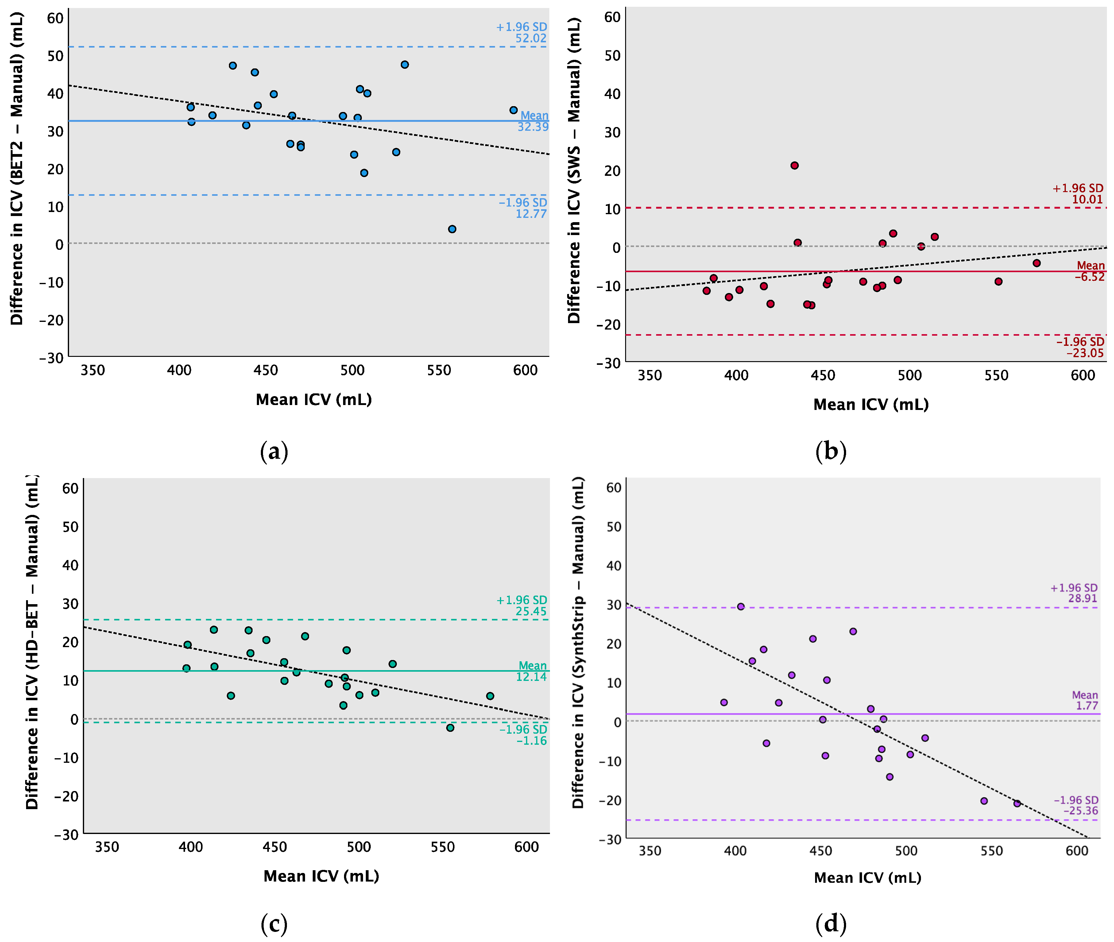
3.3.2. Intracranial Volume Estimation

Table 8 shows the ICV of the 22 premature babies scanned at TEA, estimated with the manual and automated methods. The Bland–Altman plots illustrate the agreement between the ICVs extracted from the MRI using automated segmentation methods against the reference (Figure 3). Ideally, the BE methods being compared would yield identical results, resulting in null ICV differences, but such a perfect agreement is unlikely to occur. Instead, we would expect to observe a random distribution of ICV differences clustered around zero, indicating an unbiased pattern of disagreement [71,72,73]. By examining the spread of differences both above and below zero, we can determine the extent to which the disagreement between the methods is acceptable when replacing manual for automated BE methods. If the majority of values consistently fall above/below zero, it suggests that one method consistently produces higher/lower measurements than the other. This pattern indicates that the disagreement is not random but rather systematic [71,72,73]. Furthermore, by analysing the data, we can also identify whether distinct patterns of disagreement exist among subjects with lower or higher ICVs [71,72,73].
The ICV mean differences (95% CI) or bias were as follows: 32.4 (12.8 to 52.0) mL for BET2 − Manual; −6.5 (−23.0 to 10.0) mL for SWS − Manual; 12.1 (−1.2 to 25.4) mL for HD-BET—Manual; and 1.8 (−25.4 to 28.9) mL for SynthStrip—Manual. These results can be visually perceived in some slices of Figure 2, with masks exceeding the brain area (e.g., BET2 and HD-BET) or the opposite (e.g., SWS and SynthStrip), as identified in the Bland–Altman analysis.
Most differences in the ICVs from the Bland–Altman analysis (Figure 3) were within the limits of agreement, with a range both above and below the mean difference; however, the differences were not always evenly distributed as ideally expected, so a linear regression analysis [71,73] was performed to assess the presence of proportional bias. The regression analysis was the statistical procedure used for examining the predictive relationship among the difference in ICVs between each automated and manual BE method (dependent—criterion—variable) and the mean ICV estimated by those methods (independent—predictor—variable). The results for the ICV mean differences of HD-BET—Manual (R = 0.608; p = 0.003) and SynthStrip—Manual (R = 0.719; p < 0.001) showed heteroscedasticity. However, the homoscedasticity of BET2—Manual (R = 0.317; p = 0.151) and SWS—Manual (R = 0.240; p = 0.283) did not indicate the same tendency of error with the increase in ICV. The correlational trend line of HD-BET demonstrates that for certain higher ICVs, the magnitude of positive differences tends to slightly decrease, approaching that of manual segmentation (in which the differences are closer to zero). Conversely, the regression line of SynthStrip reflects a tendency for the negative differences to increase for higher ICVs, showing a larger variability in the ICV estimations. Converting the difference between methods to percentages results in a mean bias of 6.76% for BET2; −1.42% for SWS; 2.59% for HD-BET; and 0.38% for SynthStrip. The RMSE and CVRMSE values for each automated method relative to the reference were as follows: 33.8 mL (7.31%) for BET2; 10.5 mL (2.27%) for SWS; 13.8 mL (2.99%) for HD-BET; and 13.6 mL (2.95%) for SynthStrip.

3.4. Computation Time

Each scan took roughly 3 h to segment manually. The average processing time (in seconds) for each automated BE method was as follows: 2.20 ± 0.15 (BET2); 4.95 ± 1.33 (SWS); 1288.40 ± 12.37 (HD-BET); and 266.97 ± 89.24 (SynthStrip).

4. Discussion

This study assessed different BE methods for MRI scans of preterm neonates and their effects on ICVs, showing that automated methods have a similar level of accuracy to that of manual skull stripping in T2w MRI. The study’s prerequisites were met regarding the ground truth that was created for BE, because both the intra- and inter-rater showed a high level of agreement (with average DC and ICC values above 0.980), suggesting that the full manual segmentation performed was a reliable method for establishing reference brain masks (in agreement with the findings of other studies [29,31]). Additionally, the dataset was tested as a whole, since the ICV estimation did not show significant differences in terms of gender and gestational age.
Based on the segmentation metrics results, we can interpret the different BE methods (Manual, BET2, SWS, HD-BET, and SynthStrip). According to the voxel-overlap-based metrics, HD-BET followed by SWS obtained the highest results for median DC (0.968 (IQR: 0.965–0.971) and 0.966 (IQR: 0.963–0.969)) and JC (0.938 and 0.934) values, respectively. A similar deduction can be made from the DC assessment for each brain mask subset, considering that the segmentation performance varies between them, due to anatomical differences across slices. The lower segmentation accuracy in the bottom slices might be related to the presence of different brain tissues (the cerebrum, cerebellum, and brain stem), vascular structures, air-filled cavities, and the intricate internal structure of the skull bones. The top slices cover a larger area of the brain, where it merges with the surrounding blood vessels, exterior skull bones, and scalp, challenging the segmentation of the brain from non-brain adjacent structures. HD-BET outperforms the other tested BE methods with median improvements of +0.031 (BET2), +0.002 (SWS), and +0.011 (SynthStrip) points for DC; −0.786 (BET2), −0.055 (SWS), and −0.124 (SynthStrip) mm for MSD; and −0.44 mm for HD95. Similar results were reported with HD-BET by Isensee et al. [19] with different adult MRI datasets and sequences, yielding a median DC of 0.976 (IQR, 0.970–0.980) on T1w, 0.969 (IQR, 0.961–0.974) on cT1w, 0.964 (IQR, 0.952–0.970) on FLAIR, and 0.961 (IQR, 0.952–0.967) on T2w sequences. Since SWS was not validated as a BE tool by Beare et al. [42], there are not studies comparing these results, despite their similarity to results from manual segmentation. However, the same authors proposed a BE method for T1w MRI also based on the watershed transform and validated it in human and macaque brains, showing a mean ± standard deviation DC in a pediatric cohort of 0.962 ± 0.005 [74], which is very similar to the results obtained in our study. When demonstrating the efficacy of SynthStrip, Hoopes et al. [26] included a small subset of 10 infants born full-term with T1w images acquired between 0 and 18 months, presenting similarities to our results, with a mean DC of 0.961 ± 0.014. Regarding surface-distance-based metrics, HD-BET performed well with a median HD95 of 3.2 mm (IQR: 2.5–3.6 mm), followed by SWS and SynthStrip, which also achieved good results (3.6 mm; IQR: 3.1–3.6 mm). Similar results were reported with HD-BET by Isensee et al. [19], yielding a median HD95 of 2.7 mm (IQR: 2.2–3.3 mm) on T1w, 3.2 mm (IQR: 2.8–4.1 mm) on cT1w, 4.2 mm (IQR: 3.4–5.0 mm) on FLAIR, and 4.4 mm (IQR: 3.9–5.0 mm) on T2w sequences. BET2′s overestimation of the brain boundary has also been previously reported by Smith [8]. Regarding SynthStrip, our HD95 and MSD results are better than those reported with an infant subset by Hoopes et al. [26] (38.7 ± 22.2 mm and 1.0 ± 0.3 mm, respectively) and might be related to the range of ages (0 to 18 months) included. In another study that evaluated twelve BE methods in a neonatal brain MRI dataset (preterms scanned at TEA), Serag et. al. [29] showed that the developed ALFA method [29] had a better performance than our tested methods, with a mean DC of 0.989 and an HD of 3.4 mm (for the T2w images). We intended to include this method in our study; however, it was no longer accessible, and therefore could not be tested with our dataset. Ten of the other tested methods [29] performed worse than HD-BET and SWS, namely, 3DSS (DC = 0.922), BET (DC = 0.792), BSE (DC = 0.714), LABEL (DC = 0.935), ROBEX (DC = 0.910), MV (DC = 0.951), STAPLE (DC = 0.948), SBA (DC = 0.960), BW (DC = 0.774), and BEaST (DC = 0.939). We also obtained different results when optimizing BET parameters, as Serag et. al. [29] showed a DC of 0.792, whereas in our study, it was 0.937, which is a massive improvement that suggests our parameters were better suited. The BE accuracy within a neonatal group (0.8 ± 0.3 months old) using the LABEL [31] method developed by Shi et. al. showed an average JC of 0.948 and their method performed better when compared with other BE methods (BET (JC = 0.920), BSE (JC = 0.884), ROBEX (JC = 0.886), GCUT (JC = 0.916), Majority voting (JC = 0.911), and STAPLE (JC = 0.934)). The LABEL results are slightly higher than those of HD-BET and SWS, but this could be due to the age of the dataset, since this method has a tendency for the JC to increase with the age of the sample [31]. Finally, the HSS method developed by Péporté et. al. [33] showed worse similarity metrics (DC = 0.954 and JC = 0.913) than HD-BET, SWS, and SynthStrip, as well as the other BE methods (FSL, BrainSuite, MRIcroN, and SPM8) they tested in their dataset.
Regarding ICV estimation, our Bland–Altman analysis indicated good agreement between some automated and manual BE methods, with the identification of patterns of disagreement that can be used as correction factors. BET2 consistently estimates higher ICVs than manual segmentation; this pattern is less prominent with HD-BET and with a tendency to approach to minor differences when the ICVs increase. On the other hand, SWS mostly estimates lower ICVs than manual segmentation. SynthStrip shows the largest variability, with a tendency to overestimate at lower ICVs and underestimate at higher ICVs. The ICV difference discrepancies between our study and the infant’s dataset by Hoopes et al. [26] (7.4 ± 3.5%) might be related to the wide variation in brain size between 0 and 18 months, the range of ages included in the test subset of SynthStrip. The error between automated and manual ICVs is small (<3%) for all the methods, except for BET2, indicating good agreement between the segmentation methods. However, the error obtained for BET2 was similar to that previously reported by Smith [8] when developing this widely used BE method; nonetheless, special awareness should be given when using this BE method in neonates due to the impact of a 7% measurement error when studying such small brains. SWS and HD-BET provide a level of agreement that is likely to be acceptable for experimental and clinical applications due to the smaller ICV mean differences (−6.5 mL (−1.42%) and 12.1 mL (2.59%)), median VS (2.61% and −2.03%), RMSE (10.5 mL and 13.8 mL), and CVRMSE (2.27% and 2.99%) values. This means that if the ICVs estimated from the automated BE methods are corrected by a factor of +1.42% (SWS) or −2.59% (HD-BET), it should be close to the real ICV with a small estimation error (±1.13% for SWS and ±1.49% for HD-BET). The estimates might be considered suitable considering the neonatal volume variation per week. According to Dimitrova et al. [75], 6.1% per week is a typical ICV developmental change during the neonatal period in a term-born dataset (37–45 weeks). Moreover, between 32 and 42 weeks, Mewes et al. [76] reported a brain growth of 11.2% per week. Furthermore, Gui et al. [77] and Zacharia et al. [78] depicted an average ICV growth rate of 27.2 mL and 24.0 mL per week in cohorts of premature infants that were assessed at birth and later at TEA, respectively.
Skull stripping, as a preprocessing step, should be fast, providing results that are as accurate as those of manual segmentation, which nonetheless is extremely time consuming when compared with automated methods [6,7,8,9,10,11]. Herein, we have observed that conventional automated BE methods perform faster than deep-learning-based methods, in agreement with the computation times described by other authors [9,30,53]. However, this limitation of the latter methods could be overcome by running them in GPU mode instead of CPU mode (e.g., HD-BET takes approximately 30 s in GPU mode [19]).
This study achieves the following: (1) it determines the applicability of state-of-the-art BE methods, such as HD-BET and SynthStrip, in MRI preterm infants scanned at TEA; (2) validates SWS with manual segmentation; (3) optimizes the parameters for BET2 and SynthStrip to apply in neonates; and (4) culminates in a proposal of correction factors for BE automated methods.
The current study also had some limitations, namely the dataset used for this study was small. This is because for testing the outputs of BE methods, it is recommended (1) to include the full manual segmentation as a reference, which is a time-consuming process and which is the main reason why the majority of similar studies have small sample sizes (e.g., several studies [10,12,15,16,22,29,30,33,35] reported small datasets/subgroups ranging from 5 to 22 subjects); and (2) to test subjects without detectable brain lesions or congenital conditions (and no severe motion artifacts) first [29,31,34,35,36,42], criteria which greatly limit the available datasets, as in our case, most infants had brain abnormalities.
The potential implications of these restrictions are described below:
  • The influence of our sample size on our Bland–Altman analysis [79] is difficult to determine due to the unknown clinically acceptable agreement limits for ICV measurements of preterm neonates at term. This analysis indicates the likely range of true mean differences in the specific clinical population, considering the potential for random variation [71,72,73]. Nevertheless, the findings from a small sample size are less likely to capture the characteristics and variability of the overall population, mainly when statistical inferences are applied; therefore, caution is needed when generalizing conclusions.
  • The presence of brain lesions and congenital condition or motion artifacts might lead to difficulties in accurately delineating the border between the brain and the skull, depending on their severity, location (e.g., near the border of the skull or affecting skull integrity and brain tissue characteristics), and BE method category [9]. When using BET2 [8,14], which is a deformable surface-based model approach, the presence of brain pathology and motion can pose challenges in the evolution of the mesh used to approximate the brain surface, primarily due to intensity and shape variations. However, the BE methods based on deep learning techniques are known to mitigate this constraint [9]. For instance, Isensee et al. [19] stated that HD-BET showed a robust performance in the presence of adult brain pathology- or treatment-induced tissue alterations. Additionally, Hoopes et al. [26] developed SynthStrip to be agnostic to MRI contrasts and acquisition schemes, and it was validated for age, health, resolution, and imaging modality factors. So, it is expected that deep learning methods behave similarly in a pathological neonatal context. Furthermore, motion artifacts can be present, especially in older infants, as it can be challenging to maintain their sleep during scanning [80]. Fortunately, since the typical protocols used in neonatal brain MRI (e.g., low magnetic field strengths and fast imaging sequences) do not provide high-resolution images, they are less sensitive to motion artifacts [81]. Nonetheless, special attention should be given when considering pathological cases with motion artifacts, because the performance of BE methods may vary considerably.
Concerning future work, it is recommended to expand the neonate’s dataset (with a larger sample size to increase the confidence of the findings) and perform BE in the presence of pathology, image artifacts, and different MRI protocols. Another interesting approach for further studies could be to assess regional brain volumes using pre-processed MRI scans of brains extracted with different methods.
In conclusion, HD-BET and SWS provide the best overall BE performances and can be considered, amongst the tested methods and considering our study’s limitations, the most suitable BE methods in the T2w MRI of preterm neonates scanned at TEA.

Author Contributions

Conceptualization, T.F.V. and H.A.F.; methodology, T.F.V. and H.A.F.; software, T.F.V.; validation, H.A.F. and N.C.M.; formal analysis, T.F.V. and H.A.F.; investigation, T.F.V.; resources, T.F.V., N.C.M., L.H.-W. and N.N.; data curation, T.F.V.; writing—original draft preparation, T.F.V.; writing—review and editing, T.F.V., H.A.F. and N.M.; visualization, T.F.V.; supervision, H.A.F., N.M. and N.C.M.; project administration, T.F.V., H.A.F., N.M. and N.C.M.; funding acquisition, T.F.V. All authors have read and agreed to the published version of the manuscript.

Funding

This research was supported by Fundação para a Ciência e a Tecnologia (FCT), under the IBEB Strategic Program UIDB/00645/2020 (https://doi.org/10.54499/UIDB/00645/2020), and Bolsa de Investigação para Doutoramento (2022.12483.BD).

Institutional Review Board Statement

The study was conducted in accordance with the Declaration of Helsinki, and approved by the Human Research Ethical Committee of the Medical Faculty at Uppsala University (protocol code 2014/236/1 and date of approval 24 February 2015, with one amendment 2014/236/2 dated as of 18 May 2016), and the data were included after written consent from the parents for the acquisition of images and retrospective data analysis.

Informed Consent Statement

Informed parental consent was obtained from all subjects involved in the study.

Data Availability Statement

The original dataset is unavailable due to privacy and ethical restrictions; however, the data analysed and generated are available in the main article and appendices. Further details are available on request from the corresponding author.

Conflicts of Interest

The authors declare no conflicts of interest.

Appendix A

Appendix A.1. BET2 Parameters

To define the parameters for the brain extraction (BE) of neonatal studies, BET2 from FSL version 6.0.6.4 [8,14,44] was tested with modified options from the BET2 program:
  • Fractional intensity threshold (<f> parameter varied from 0 to 1 in steps of 0.05; 0.50 is the default value), where smaller values results in larger brain outline estimates, and higher values result in smaller brain outline estimates.
  • Vertical gradient in fractional intensity threshold (<g> parameter varied from −1 to 1 in steps of 0.05; 0 is the default value), where positive values result in a larger brain outline at the bottom and a smaller one at the top of the scale, and negative values result in the opposite.
  • Robust brain centre estimation (<R>), iterates BET2 several times with the purpose of improving the BE, when the input data contains a considerable amount of non-brain matter.
  • Eye and optic nerve cleanup (<S>) attempts to clean up the residual eye and optic nerve voxels that are remaining after running standard BE using BET2.
  • Bias field and neck cleanup (<B>) attempts to reduce image bias and residual neck voxels after running standard BE using BET2.
Only one of the options (<R>, <S>, and <B>) can be selected for each BET2 run, together with <f> and <g>.
The extracted brain images were assessed for quality (i.e., an accurate brain outline, excluding voxels from the eyes, optic nerve, neck, arms, and hands in the neonatal MRI) and according to the dice coefficient (DC) score results, after comparing the results to those with manual segmentation.
After testing all the options, the options (<f> from 0.50 to 0.60 and <g> from −0.10 to 0.20) that provided higher DC scores were pre-selected to perform a further analysis (Figure A1). The DC scores were tested for general differences with the Friedman test (χ2 (20) = 376.364, p < 0.001). For post hoc comparisons, Bonferroni-adjusted significance tests were used for pairwise comparisons.
Figure A1. Dice coefficients with varying BET2 options per subject (n = 22 premature neonates, each one represented by different color lines).
Applsci 14 01339 g0a1
The parameters <f> 0.6 and <g> 0.1 were used for all the neonates’ MRI images, as they provided the best DC score (0.936 ± 0.006) and showed no statistically significant differences when compared with other options that also provided high DC scores (>0.931). Including the option <R> also provided good results, without statistically significant differences (paired samples t-test: t(9) = 1.899; p = 0.071), but since this option generally runs slower (4.87 ± 0.37 s) compared with the standard (2.20 ± 0.15 s), it was not considered further.

Appendix A.2. SynthStrip Parameters

The BE tool from SynthStrip [26] allows for the fine-tuning of the mask boundary distance from the brain (<b>, 1 mm is the default value). This option was varied from −2 to 3 mm in steps of 1 mm. The extracted brain images were compared with manual segmentation through DC metrics.
The DC were tested for general differences with a repeated measures ANOVA (F(1.066, 22.396) = 50.975, p < 0.001, partial η2 = 0.708). For post hoc comparisons, Bonferroni-adjusted significance tests were used for pairwise comparisons.
The mask border threshold of 0 and 1 mm provided the highest DC (0.958 ± 0.005 and 0.956 ± 0.008, respectively) and there were no statistically significant differences between them (p = 1.000), so in order to simplify processes, the default value (1 mm) was applied to all the neonates’ MRI scans.
All statistical analyses were performed considering a significance value of 5% and using the IBM® SPSS® v27 software.

Appendix B

Table A1. List of segmentation metrics with respective equations and descriptions used for assessment of brain extraction methods.
MetricsEquationsDescription
Voxel-overlap-based metricsDice Coefficient (DC) [69,70,82,83,84] D C = 2 | M A | M + | A | = 2 T P 2 T P + F P + F N DC describes the similarity level between the segmentation results (i.e., brain masks obtained with different automatic brain extraction methods) and ground truth (i.e., manual segmentation). It ranges from 0 (no overlap) to 1 (perfect match). DC is the most frequently used metric for accurate analysis of brain extraction and is also known as F1 score/measure or overlap index.
Jaccard Coefficient (JC) [69,70,84,85] J C = | M A | | M A | = T P T P + F P + F N JC is defined as the intersection between the automatic segmentation and the manual segmentation over their union. It ranges from 0 (no intersection) to 1 (full intersection). It is similar to DC regarding the measurement aspects and ranking.
Precision (Pr) [69,70,84] P r = | M A | | A | = T P T P + F P Pr is also called the positive predictive value (PPV) or confidence. It is defined as the amount of overlap with respect to the automatic segmentation.
Sensitivity (Se) [69,70,84] S e = | M A | | M | = T P T P + F N Se is also called recall or true positive rate (TPR). It is defined as the amount of overlap with respect to manual segmentation.
Specificity (Sp) [69,70,84] S p = | M ¯ A ¯ | | M ¯ | = T N T N + F P Sp is also called true negative rate (TNR). It is defined as the fraction of pixels correctly labelled as “background” (i.e., non-brain tissue).
False Positive Rate (FPR) [69,70,84] F P R = | A M | | M | = F P T N + F P = 1 S p FPR is also called fallout. It can be considered an estimation of over-segmentation, indicating how many pixels identified as brain, by the automatic method, are outside of the manual mask.
False Negative Rate (FNR) [69,70,84] F N R = | M A | | M | = F N T P + F N = 1 S e FNR is also called miss rate. It can be considered an estimation of under-segmentation, indicating the falsely segmented pixels over the total number of pixels in manual segmentation.
Volume-based metricsVolume Similarity (VS) [70,86] V S = 2 V A u t V M a n V A u t + V M a n 100 ( % ) VS represents the volume size difference (as a percentage) between the automatic and manual segmentations, whilst the overlap between brain masks is not considered. A negative VS means the volume is underestimated, and a positive VS means the volume is overestimated.
Root Mean Square Error (RMSE) [87] R M S E = 1 n i = 1 n ( V A u t , i V M a n , i ) 2 RMSE measures the volume (mL) deviations between the automatic and manual segmentations. It is the square root of the mean square error. A smaller RMSE value means better volume agreement between methods.
Coefficient of Variation of the Root Mean Square Error (CVRMSE) [87] C V R M S E = R M S E V M a n ¯ 100 CVRMSE is also called normalized RMSE or percent RMS. Normalizing the RMSE by the mean value of the manual volume provides the coefficient of variation (%) of the automated volumes relative to the manual volumes.
Surface distance-based metricsHausdorff Distance (HD) [69,70,88,89] H D ( S A u t , S M a n ) = m a x { d S A u t , S M a n , d ( S M a n , S A u t ) }
where
d ( S A u t , S M a n ) = max s aut S Aut m i n s m a n S M a n s a u t s m a n
HD measures the spatial consistency of the overlap between the automatic and manual segmentations by measuring the maximum surface-to-surface distance between the two brain masks. A smaller HD indicates a higher similarity between brain masks.
Hausdorff Distance 95% Percentile (HD95) [69,70,90] H D ( S A u t , S M a n ) = P 0.95 { d S A u t , S M a n , d ( S M a n , S A u t ) } HD95 is similar to the maximum HD but considers only the 95th percentile of the distances in order to overcome the impact of outliers.
Mean Surface Distance (MSD) [69,89] M S D = 1 S A u t + S M a n s a u t S A u t d s a u t , S M a n + s m a n S M a n d s m a n , S A u t MSD represents the average of all of the distances from pixels on the boundary of the automatic segmentation to the boundary of the manual segmentation, and vice versa.
Median Surface Distance (MDSD) [86] M D S D = m e d i a n d s a u t , S M a n , s m a n , S A u t MDSD represents the median of all of the distances from pixels on the boundary of the automatic segmentation to the boundary of the manual segmentation, and vice versa.
Standard Deviation Surface Distance (STDSD) [69,89] S T D S D = 1 S A u t + S M a n s a u t S A u t d s a u t , S M a n M S D 2 + s m a n S M a n d s m a n , S A u t M S D 2 STDSD represents the standard deviation of all of the distances from pixels on the boundary of the automatic segmentation to the boundary of the manual segmentation, and vice versa.
M and A stand for the number of pixels inside the brain mask obtained from manual and automatic segmentations, respectively. V M a n and V A u t stand for the volume obtained from manual and automatic segmentations, respectively. n stands for the sample size. d S M a n , S A u t stands for the Euclidean distance between corresponding paired points in S M a n and S A u t . S M a n and S A u t stand for the surface pixels of brain mask obtained from manual and automatic segmentations, respectively. True positive (TP), true negative (TN), false positive (FP), and false negative (FN) reflect the number of pixels in the automatic segmentation that are classified correctly (true) or incorrectly (false) with respect to the manual segmentation.

Appendix C

Figure A2. Comparison of segmentation metrics ((a) DC, (b) JC, (c) Pr, (d) Se, (e) Sp, (f) FPR, (g) FNR, (h) VS, (i) HD, (j) HD95, (k) MSD, (l) MDSD) between the four automated brain extraction methods using violin plots (with box plots inside and data points on the side).
Applsci 14 01339 g0a2aApplsci 14 01339 g0a2b

References

  1. Volpe, J.J. Neurology of the Newborn, 5th ed.; Saunders: Philadelphia, PA, USA, 2008; pp. 172–177. [Google Scholar]
  2. Rutherford, M.A. Imaging the Neonatal Brain. In The Newborn Brain; Lagercrantz, H., Hanson, M.A., Ment, L.R., Peebles, D.M., Eds.; Cambridge University Press: Cambridge, UK, 2010; pp. 199–210. ISBN 978-0-511-71184-8. [Google Scholar]
  3. Dubois, J.; Alison, M.; Counsell, S.J.; Hertz-Pannier, L.; Hüppi, P.S.; Benders, M.J.N.L. MRI of the Neonatal Brain: A Review of Methodological Challenges and Neuroscientific Advances. J. Magn. Reason. Imaging 2021, 53, 1318–1343. [Google Scholar] [CrossRef]
  4. British Association of Perinatal Medicine. Neonatal Brain Magnetic Resonance Imaging: Clinical Indications, Acquisition and Reporting. 2023. Available online: https://www.bapm.org/resources/neonatal-brain-magnetic-resonance-imaging (accessed on 30 November 2023).
  5. Li, G.; Wang, L.; Yap, P.-T.; Wang, F.; Wu, Z.; Meng, Y.; Dong, P.; Kim, J.; Shi, F.; Rekik, I.; et al. Computational Neuroanatomy of Baby Brains: A Review. NeuroImage 2019, 185, 906–925. [Google Scholar] [CrossRef]
  6. Devi, C.N.; Chandrasekharan, A.; Sundararaman, V.K.; Alex, Z.C. Neonatal Brain MRI Segmentation: A Review. Comput. Biol. Med. 2015, 64, 163–178. [Google Scholar] [CrossRef]
  7. Kalavathi, P.; Prasath, V.B.S. Methods on Skull Stripping of MRI Head Scan Images—A Review. J. Digit. Imaging 2016, 29, 365–379. [Google Scholar] [CrossRef]
  8. Smith, S.M. Fast Robust Automated Brain Extraction. Hum. Brain Mapp. 2002, 17, 143–155. [Google Scholar] [CrossRef]
  9. Fatima, A.; Shahid, A.R.; Raza, B.; Madni, T.M.; Janjua, U.I. State-of-the-Art Traditional to the Machine- and Deep-Learning-Based Skull Stripping Techniques, Models, and Algorithms. J. Digit. Imaging 2020, 33, 1443–1464. [Google Scholar] [CrossRef]
  10. Mahapatra, D. Skull Stripping of Neonatal Brain MRI: Using Prior Shape Information with Graph Cuts. J. Digit. Imaging 2012, 25, 802–814. [Google Scholar] [CrossRef]
  11. Makropoulos, A.; Counsell, S.J.; Rueckert, D. A Review on Automatic Fetal and Neonatal Brain MRI Segmentation. NeuroImage 2018, 170, 231–248. [Google Scholar] [CrossRef]
  12. Eskildsen, S.F.; Coupé, P.; Fonov, V.; Manjón, J.V.; Leung, K.K.; Guizard, N.; Wassef, S.N.; Østergaard, L.R.; Collins, D.L.; Alzheimer’s Disease Neuroimaging Initiative. BEaST: Brain Extraction Based on Nonlocal Segmentation Technique. NeuroImage 2012, 59, 2362–2373. [Google Scholar] [CrossRef]
  13. Rex, D.E.; Shattuck, D.W.; Woods, R.P.; Narr, K.L.; Luders, E.; Rehm, K.; Stoltzner, S.E.; Rottenberg, D.A.; Toga, A.W. A Meta-Algorithm for Brain Extraction in MRI. NeuroImage 2004, 23, 625–637. [Google Scholar] [CrossRef]
  14. Jenkinson, M.; Pechaud, M.; Smith, S. BET2: MR-Based Estimation of Brain, Skull and Scalp Surfaces. In Proceedings of the Eleventh Annual Meeting of the Organization for Human Brain Mapping, Toronto, ON, Canada, 12–16 June 2005. [Google Scholar]
  15. Shattuck, D.W.; Sandor-Leahy, S.R.; Schaper, K.A.; Rottenberg, D.A.; Leahy, R.M. Magnetic Resonance Image Tissue Classification Using a Partial Volume Model. NeuroImage 2001, 13, 856–876. [Google Scholar] [CrossRef]
  16. Lucena, O.; Souza, R.; Rittner, L.; Frayne, R.; Lotufo, R. Convolutional Neural Networks for Skull-Stripping in Brain MR Imaging Using Silver Standard Masks. Artif. Intell. Med. 2019, 98, 48–58. [Google Scholar] [CrossRef]
  17. Kleesiek, J.; Urban, G.; Hubert, A.; Schwarz, D.; Maier-Hein, K.; Bendszus, M.; Biller, A. Deep MRI Brain Extraction: A 3D Convolutional Neural Network for Skull Stripping. NeuroImage 2016, 129, 460–469. [Google Scholar] [CrossRef] [PubMed]
  18. Ségonne, F.; Dale, A.M.; Busa, E.; Glessner, M.; Salat, D.; Hahn, H.K.; Fischl, B. A Hybrid Approach to the Skull Stripping Problem in MRI. NeuroImage 2004, 22, 1060–1075. [Google Scholar] [CrossRef] [PubMed]
  19. Isensee, F.; Schell, M.; Pflueger, I.; Brugnara, G.; Bonekamp, D.; Neuberger, U.; Wick, A.; Schlemmer, H.-P.; Heiland, S.; Wick, W.; et al. Automated Brain Extraction of Multisequence MRI Using Artificial Neural Networks. Hum. Brain Mapp. 2019, 40, 4952–4964. [Google Scholar] [CrossRef]
  20. Doshi, J.; Erus, G.; Ou, Y.; Gaonkar, B.; Davatzikos, C. Multi-Atlas Skull-Stripping. Acad. Radiol. 2013, 20, 1566–1576. [Google Scholar] [CrossRef]
  21. Rehm, K.; Schaper, K.; Anderson, J.; Woods, R.; Stoltzner, S.; Rottenberg, D. Putting Our Heads Together: A Consensus Approach to Brain/Non-Brain Segmentation in T1-Weighted MR Volumes. NeuroImage 2004, 22, 1262–1270. [Google Scholar] [CrossRef]
  22. Iglesias, J.E.; Liu, C.-Y.; Thompson, P.M.; Tu, Z. Robust Brain Extraction across Datasets and Comparison with Publicly Available Methods. IEEE Trans. Med. Imaging 2011, 30, 1617–1634. [Google Scholar] [CrossRef]
  23. Roy, S.; Butman, J.A.; Pham, D.L. Robust Skull Stripping Using Multiple MR Image Contrasts Insensitive to Pathology. NeuroImage 2017, 146, 132–147. [Google Scholar] [CrossRef]
  24. Rohlfing, T.; Maurer, C.R. Shape-Based Averaging. IEEE Trans. Image Process. 2007, 16, 153–161. [Google Scholar] [CrossRef]
  25. Carass, A.; Cuzzocreo, J.; Wheeler, M.B.; Bazin, P.-L.; Resnick, S.M.; Prince, J.L. Simple Paradigm for Extra-Cerebral Tissue Removal: Algorithm and Analysis. NeuroImage 2011, 56, 1982–1992. [Google Scholar] [CrossRef]
  26. Hoopes, A.; Mora, J.S.; Dalca, A.V.; Fischl, B.; Hoffmann, M. SynthStrip: Skull-Stripping for Any Brain Image. NeuroImage 2022, 260, 119474. [Google Scholar] [CrossRef]
  27. Cox, R.W. AFNI: Software for Analysis and Visualization of Functional Magnetic Resonance Neuroimages. Comput. Biomed. Res. 1996, 29, 162–173. [Google Scholar] [CrossRef]
  28. Hwang, H.; Rehman, H.Z.U.; Lee, S. 3D U-Net for Skull Stripping in Brain MRI. Appl. Sci. 2019, 9, 569. [Google Scholar] [CrossRef]
  29. Serag, A.; Blesa, M.; Moore, E.J.; Pataky, R.; Sparrow, S.A.; Wilkinson, A.G.; Macnaught, G.; Semple, S.I.; Boardman, J.P. Accurate Learning with Few Atlases (ALFA): An Algorithm for MRI Neonatal Brain Extraction and Comparison with 11 Publicly Available Methods. Sci. Rep. 2016, 6, 23470. [Google Scholar] [CrossRef]
  30. Wang, L.; Wu, Z.; Chen, L.; Sun, Y.; Lin, W.; Li, G. iBEAT V2.0: A Multisite-Applicable, Deep Learning-Based Pipeline for Infant Cerebral Cortical Surface Reconstruction. Nat. Protoc. 2023, 18, 1488–1509. [Google Scholar] [CrossRef]
  31. Shi, F.; Wang, L.; Dai, Y.; Gilmore, J.H.; Lin, W.; Shen, D. LABEL: Pediatric Brain Extraction Using Learning-Based Meta-Algorithm. NeuroImage 2012, 62, 1975–1986. [Google Scholar] [CrossRef]
  32. Warfield, S.K.; Zou, K.H.; Wells, W.M. Simultaneous Truth and Performance Level Estimation (STAPLE): An Algorithm for the Validation of Image Segmentation. IEEE Trans. Med. Imaging 2004, 23, 903–921. [Google Scholar] [CrossRef]
  33. Péporté, M.; Ilea Ghita, D.E.; Twomey, E.; Whelan, P.F. A Hybrid Approach to Brain Extraction from Premature Infant MRI. In Lecture Notes in Computer Science, Proceedings of the Image Analysis: 17th Scandinavian Conference, SCIA 2011, Ystad, Sweden, 23–25 May 2011; Heyden, A., Kahl, F., Eds.; Springer: Berlin/Heidelberg, Germany, 2011; Volume 6688, pp. 719–730. [Google Scholar]
  34. Yamaguchi, K.; Fujimoto, Y.; Kobashi, S.; Wakata, Y.; Ishikura, R.; Kuramoto, K.; Imawaki, S.; Hirota, S.; Hata, Y. Automated Fuzzy Logic Based Skull Stripping in Neonatal and Infantile MR Images. In Proceedings of the International Conference on Fuzzy Systems, Barcelona, Spain, 18–23 July 2010; pp. 1–7. [Google Scholar]
  35. Kobashi, S.; Udupa, J.K. Fuzzy Connectedness Image Segmentation for Newborn Brain Extraction in MR Images. In Proceedings of the 35th Annual International Conference of the IEEE Engineering in Medicine and Biology Society (EMBC), Osaka, Japan, 3–7 July 2013; pp. 7136–7139. [Google Scholar]
  36. Gousias, I.S.; Edwards, A.D.; Rutherford, M.A.; Counsell, S.J.; Hajnal, J.V.; Rueckert, D.; Hammers, A. Magnetic Resonance Imaging of the Newborn Brain: Manual Segmentation of Labelled Atlases in Term-Born and Preterm Infants. Neuroimage 2012, 62, 1499–1509. [Google Scholar] [CrossRef]
  37. Plaisier, A.; Govaert, P.; Lequin, M.H.; Dudink, J. Optimal Timing of Cerebral MRI in Preterm Infants to Predict Long-Term Neurodevelopmental Outcome: A Systematic Review. AJNR Am. J. Neuroradiol. 2014, 35, 841–847. [Google Scholar] [CrossRef]
  38. Fedorov, A.; Beichel, R.; Kalpathy-Cramer, J.; Finet, J.; Fillion-Robin, J.-C.; Pujol, S.; Bauer, C.; Jennings, D.; Fennessy, F.; Sonka, M.; et al. 3D Slicer as an Image Computing Platform for the Quantitative Imaging Network. Magn. Reason. Imaging 2012, 30, 1323–1341. [Google Scholar] [CrossRef]
  39. Eritaia, J.; Wood, S.J.; Stuart, G.W.; Bridle, N.; Dudgeon, P.; Maruff, P.; Velakoulis, D.; Pantelis, C. An Optimized Method for Estimating Intracranial Volume from Magnetic Resonance Images. Magn. Reson. Med. 2000, 44, 973–977. [Google Scholar] [CrossRef]
  40. Mai, J.; Majtanik, M.; Paxinos, G. Atlas of the Human Brain, 4th ed.; Academic Press: Cambridge, MA, USA, 2015; pp. 7–40. [Google Scholar]
  41. Griffiths, P.D.; Morris, J.; Larroche, J.-C.; Reeves, M. Atlas of Fetal and Postnatal Brain MR Imaging, 1st ed.; Mosby: Philadelphia, PA, USA, 2010; pp. 35–157. [Google Scholar]
  42. Beare, R.J.; Chen, J.; Kelly, C.E.; Alexopoulos, D.; Smyser, C.D.; Rogers, C.E.; Loh, W.Y.; Matthews, L.G.; Cheong, J.L.Y.; Spittle, A.J.; et al. Neonatal Brain Tissue Classification with Morphological Adaptation and Unified Segmentation. Front. Neuroinform. 2016, 10, 12. [Google Scholar] [CrossRef]
  43. Merkel, D. Docker: Lightweight Linux Containers for Consistent Development and Deployment. Linux J. 2014, 239, 2. [Google Scholar]
  44. Jenkinson, M.; Beckmann, C.F.; Behrens, T.E.J.; Woolrich, M.W.; Smith, S.M. FSL. NeuroImage 2012, 62, 782–790. [Google Scholar] [CrossRef]
  45. Penny, W.D.; Friston, K.J.; Ashburner, J.T.; Kiebel, S.J.; Nichols, T.E. Statistical Parametric Mapping: The Analysis of Functional Brain Images, 1st ed.; Academic Press: Cambridge, MA, USA, 2006; p. 689. [Google Scholar]
  46. MATLAB Version: 9.14.0 (R2023a); The MathWorks Inc.: Natick, MA, USA, 2023.
  47. Fischl, B. FreeSurfer. NeuroImage 2012, 62, 774–781. [Google Scholar] [CrossRef]
  48. Alexander, B.; Kelly, C.E.; Adamson, C.; Beare, R.; Zannino, D.; Chen, J.; Murray, A.L.; Loh, W.Y.; Matthews, L.G.; Warfield, S.K.; et al. Changes in Neonatal Regional Brain Volume Associated with Preterm Birth and Perinatal Factors. NeuroImage 2019, 185, 654–663. [Google Scholar] [CrossRef]
  49. Thompson, D.K.; Kelly, C.E.; Chen, J.; Beare, R.; Alexander, B.; Seal, M.L.; Lee, K.J.; Matthews, L.G.; Anderson, P.J.; Doyle, L.W.; et al. Characterisation of Brain Volume and Microstructure at Term-Equivalent Age in Infants Born across the Gestational Age Spectrum. Neuroimage Clin. 2019, 21, 101630. [Google Scholar] [CrossRef]
  50. Alexander, B.; Loh, W.Y.; Matthews, L.G.; Murray, A.L.; Adamson, C.; Beare, R.; Chen, J.; Kelly, C.E.; Anderson, P.J.; Doyle, L.W.; et al. Desikan-Killiany-Tourville Atlas Compatible Version of M-CRIB Neonatal Parcellated Whole Brain Atlas: The M-CRIB 2.0. Front. Neurosci. 2019, 13, 34. [Google Scholar] [CrossRef]
  51. Thompson, D.K.; Kelly, C.E.; Chen, J.; Beare, R.; Alexander, B.; Seal, M.L.; Lee, K.; Matthews, L.G.; Anderson, P.J.; Doyle, L.W.; et al. Early Life Predictors of Brain Development at Term-Equivalent Age in Infants Born across the Gestational Age Spectrum. NeuroImage 2019, 185, 813–824. [Google Scholar] [CrossRef]
  52. Kelly, C.E.; Thompson, D.K.; Spittle, A.J.; Chen, J.; Seal, M.L.; Anderson, P.J.; Doyle, L.W.; Cheong, J.L.Y. Regional Brain Volumes, Microstructure and Neurodevelopment in Moderate-Late Preterm Children. Arch. Dis. Child.-Fetal Neonatal Ed. 2020, 105, 593–599. [Google Scholar] [CrossRef]
  53. Ding, Y.; Acosta, R.; Enguix, V.; Suffren, S.; Ortmann, J.; Luck, D.; Dolz, J.; Lodygensky, G.A. Using Deep Convolutional Neural Networks for Neonatal Brain Image Segmentation. Front. Neurosci. 2020, 14, 207. [Google Scholar] [CrossRef]
  54. Alexander, B.; Yang, J.Y.-M.; Yao, S.H.W.; Wu, M.H.; Chen, J.; Kelly, C.E.; Ball, G.; Matthews, L.G.; Seal, M.L.; Anderson, P.J.; et al. White Matter Extension of the Melbourne Children’s Regional Infant Brain Atlas: M-CRIB-WM. Hum. Brain Mapp. 2020, 41, 2317–2333. [Google Scholar] [CrossRef]
  55. Mongerson, C.R.L.; Wilcox, S.L.; Goins, S.M.; Pier, D.B.; Zurakowski, D.; Jennings, R.W.; Bajic, D. Infant Brain Structural MRI Analysis in the Context of Thoracic Non-Cardiac Surgery and Critical Care. Front. Pediatr. 2019, 7, 315. [Google Scholar] [CrossRef]
  56. Collins, S.E.; Thompson, D.K.; Kelly, C.E.; Gilchrist, C.P.; Matthews, L.G.; Pascoe, L.; Lee, K.J.; Inder, T.E.; Doyle, L.W.; Cheong, J.L.Y.; et al. Development of Regional Brain Gray Matter Volume across the First 13 Years of Life Is Associated with Childhood Math Computation Ability for Children Born Very Preterm and Full Term. Brain Cogn. 2022, 160, 105875. [Google Scholar] [CrossRef]
  57. Treyvaud, K.; Thompson, D.; Kelly, C.; Loh, W.; Inder, T.; Cheong, J.; Doyle, L.; Anderson, P. Early Parenting Is Associated with the Developing Brains of Children Born Very Preterm. Clin. Neuropsychol. 2021, 35, 885–903. [Google Scholar] [CrossRef]
  58. Monson, B.B.; Anderson, P.J.; Matthews, L.G.; Neil, J.J.; Kapur, K.; Cheong, J.L.Y.; Doyle, L.W.; Thompson, D.K.; Inder, T.E. Examination of the Pattern of Growth of Cerebral Tissue Volumes From Hospital Discharge to Early Childhood in Very Preterm Infants. JAMA Pediatr. 2016, 170, 772–779. [Google Scholar] [CrossRef]
  59. Granger, C.; Spittle, A.J.; Walsh, J.; Pyman, J.; Anderson, P.J.; Thompson, D.K.; Lee, K.J.; Coleman, L.; Dagia, C.; Doyle, L.W.; et al. Histologic Chorioamnionitis in Preterm Infants: Correlation with Brain Magnetic Resonance Imaging at Term Equivalent Age. BMC Pediatr. 2018, 18, 63. [Google Scholar] [CrossRef]
  60. Strahle, J.M.; Triplett, R.L.; Alexopoulos, D.; Smyser, T.A.; Rogers, C.E.; Limbrick, D.D.; Smyser, C.D. Impaired Hippocampal Development and Outcomes in Very Preterm Infants with Perinatal Brain Injury. NeuroImage Clin. 2019, 22, 101787. [Google Scholar] [CrossRef]
  61. Matthews, L.G.; Smyser, C.D.; Cherkerzian, S.; Alexopoulos, D.; Kenley, J.; Tuuli, M.G.; Michael Nelson, D.; Inder, T.E. Maternal Pomegranate Juice Intake and Brain Structure and Function in Infants with Intrauterine Growth Restriction: A Randomized Controlled Pilot Study. PLoS ONE 2019, 14, e0219596. [Google Scholar] [CrossRef]
  62. Rudisill, S.S.; Wang, J.T.; Jaimes, C.; Mongerson, C.R.L.; Hansen, A.R.; Jennings, R.W.; Bajic, D. Neurologic Injury and Brain Growth in the Setting of Long-Gap Esophageal Atresia Perioperative Critical Care: A Pilot Study. Brain Sci. 2019, 9, 383. [Google Scholar] [CrossRef]
  63. Vanderhasselt, T.; Naeyaert, M.; Watté, N.; Allemeersch, G.-J.; Raeymaeckers, S.; Dudink, J.; de Mey, J.; Raeymaekers, H. Synthetic MRI of Preterm Infants at Term-Equivalent Age: Evaluation of Diagnostic Image Quality and Automated Brain Volume Segmentation. AJNR Am. J. Neuroradiol. 2020, 41, 882–888. [Google Scholar] [CrossRef]
  64. GilchristKelly, C.P.; Thompson, D.K.; Alexander, B.; Kelly, C.E.; Treyvaud, K.; Matthews, L.G.; Pascoe, L.; Zannino, D.; Yates, R.; Adamson, C.; et al. Growth of Prefrontal and Limbic Brain Regions and Anxiety Disorders in Children Born Very Preterm. Psychol. Med. 2023, 53, 759–770. [Google Scholar] [CrossRef]
  65. Bell, K.A.; Cherkerzian, S.; Drouin, K.; Matthews, L.G.; Inder, T.E.; Prohl, A.K.; Warfield, S.K.; Belfort, M.B. Associations of Macronutrient Intake Determined by Point-of-Care Human Milk Analysis with Brain Development among Very Preterm Infants. Children 2022, 9, 969. [Google Scholar] [CrossRef]
  66. Whitwell, J.L.; Crum, W.R.; Watt, H.C.; Fox, N.C. Normalization of Cerebral Volumes by Use of Intracranial Volume: Implications for Longitudinal Quantitative MR Imaging. Am. J. Neuroradiol. 2001, 22, 1483–1489. [Google Scholar]
  67. Van Rossum, G.; Drake, F.L. Python 3 Reference Manual; CreateSpace: Scotts Valley, CA, USA, 2009. [Google Scholar]
  68. IBM Corp. IBM SPSS Statistics for Windows; Version 27.0; IBM Corp: Armonk, NY, USA, 2020. [Google Scholar]
  69. Yeghiazaryan, V.; Voiculescu, I. Family of Boundary Overlap Metrics for the Evaluation of Medical Image Segmentation. J. Med. Imaging 2018, 5, 015006. [Google Scholar] [CrossRef]
  70. Taha, A.A.; Hanbury, A. Metrics for Evaluating 3D Medical Image Segmentation: Analysis, Selection, and Tool. BMC Med. Imaging 2015, 15, 29. [Google Scholar] [CrossRef]
  71. Portney, L.G. Foundations of Clinical Research: Applications to Evidence-Based Practice, 4th ed.; FA Davis: Philadelphia, PA, USA, 2020; ISBN 978-0-8036-6113-4. [Google Scholar]
  72. Bland, J.M.; Altman, D.G. Statistical Methods for Assessing Agreement between Two Methods of Clinical Measurement. Lancet 1986, 1, 307–310. [Google Scholar] [CrossRef]
  73. Bland, J.M.; Altman, D.G. Measuring Agreement in Method Comparison Studies. Stat. Methods Med. Res. 1999, 8, 135–160. [Google Scholar] [CrossRef]
  74. Beare, R.; Chen, J.; Adamson, C.L.; Silk, T.; Thompson, D.K.; Yang, J.Y.M.; Anderson, V.A.; Seal, M.L.; Wood, A.G. Brain Extraction Using the Watershed Transform from Markers. Front. Neuroinform. 2013, 7, 32. [Google Scholar] [CrossRef]
  75. Dimitrova, R.; Arulkumaran, S.; Carney, O.; Chew, A.; Falconer, S.; Ciarrusta, J.; Wolfers, T.; Batalle, D.; Cordero-Grande, L.; Price, A.N.; et al. Phenotyping the Preterm Brain: Characterizing Individual Deviations From Normative Volumetric Development in Two Large Infant Cohorts. Cerebral Cortex 2021, 31, 3665–3677. [Google Scholar] [CrossRef]
  76. Mewes, A.U.J.; Hüppi, P.S.; Als, H.; Rybicki, F.J.; Inder, T.E.; McAnulty, G.B.; Mulkern, R.V.; Robertson, R.L.; Rivkin, M.J.; Warfield, S.K. Regional Brain Development in Serial Magnetic Resonance Imaging of Low-Risk Preterm Infants. Pediatrics 2006, 118, 23–33. [Google Scholar] [CrossRef] [PubMed]
  77. Gui, L.; Loukas, S.; Lazeyras, F.; Hüppi, P.S.; Meskaldji, D.E.; Borradori Tolsa, C. Longitudinal Study of Neonatal Brain Tissue Volumes in Preterm Infants and Their Ability to Predict Neurodevelopmental Outcome. Neuroimage 2019, 185, 728–741. [Google Scholar] [CrossRef]
  78. Zacharia, A.; Zimine, S.; Lovblad, K.O.; Warfield, S.; Thoeny, H.; Ozdoba, C.; Bossi, E.; Kreis, R.; Boesch, C.; Schroth, G.; et al. Early Assessment of Brain Maturation by MR Imaging Segmentation in Neonates and Premature Infants. AJNR Am. J. Neuroradiol. 2006, 27, 972–977. [Google Scholar]
  79. Lu, M.-J.; Zhong, W.-H.; Liu, Y.-X.; Miao, H.-Z.; Li, Y.-C.; Ji, M.-H. Sample Size for Assessing Agreement between Two Methods of Measurement by Bland-Altman Method. Int. J. Biostat. 2016, 12, 20150039. [Google Scholar] [CrossRef]
  80. Howell, B.R.; Styner, M.A.; Gao, W.; Yap, P.-T.; Wang, L.; Baluyot, K.; Yacoub, E.; Chen, G.; Potts, T.; Salzwedel, A.; et al. The UNC/UMN Baby Connectome Project (BCP): An Overview of the Study Design and Protocol Development. Neuroimage 2019, 185, 891–905. [Google Scholar] [CrossRef]
  81. Havsteen, I.; Ohlhues, A.; Madsen, K.H.; Nybing, J.D.; Christensen, H.; Christensen, A. Are Movement Artifacts in Magnetic Resonance Imaging a Real Problem?—A Narrative Review. Front. Neurol. 2017, 8, 232. [Google Scholar] [CrossRef]
  82. Sørensen, T. A Method of Establishing Groups of Equal Amplitude in Plant Sociology Based on Similarity of Species Content and Its Application to Analyses of the Vegetation on Danish Commons. K. Dan. Vidensk. Selsk. 1948, 5, 1–34. [Google Scholar]
  83. Dice, L.R. Measures of the Amount of Ecologic Association Between Species. Ecology 1945, 26, 297–302. [Google Scholar] [CrossRef]
  84. Powers, D.M.W. Evaluation: From Precision, Recall and F-Measure to ROC, Informedness, Markedness and Correlation. Int. J. Mach. Learn. 2011, 2, 37–63. [Google Scholar] [CrossRef]
  85. Jaccard, P. The Distribution of the Flora in the Alpine Zone. New Phytol. 1912, 11, 37–50. [Google Scholar] [CrossRef]
  86. Segmentation Evaluation. Available online: http://insightsoftwareconsortium.github.io/SimpleITK-Notebooks/Python_html/34_Segmentation_Evaluation.html (accessed on 26 August 2023).
  87. Root-Mean-Square Deviation. Wikipedia. 2023. Available online: https://en.wikipedia.org/w/index.php?title=Root-mean-square_deviation&oldid=1171599164 (accessed on 16 September 2023).
  88. Birsan, T.; Tiba, D. One Hundred Years Since the Introduction of the Set Distance by Dimitrie Pompeiu. In System Modeling and Optimization: Proceedings of the 22nd IFIP TC7 Conference, Turin, Italy, 18–22 July 2005; Ceragioli, F., Dontchev, A., Futura, H., Marti, K., Pandolfi, L., Eds.; Springer: Boston, MA, USA, 2006; pp. 35–39. [Google Scholar]
  89. Heimann, T.; van Ginneken, B.; Styner, M.A.; Arzhaeva, Y.; Aurich, V.; Bauer, C.; Beck, A.; Becker, C.; Beichel, R.; Bekes, G.; et al. Comparison and Evaluation of Methods for Liver Segmentation From CT Datasets. IEEE Trans. Med. Imaging 2009, 28, 1251–1265. [Google Scholar] [CrossRef]
  90. Menze, B.H.; Jakab, A.; Bauer, S.; Kalpathy-Cramer, J.; Farahani, K.; Kirby, J.; Burren, Y.; Porz, N.; Slotboom, J.; Wiest, R.; et al. The Multimodal Brain Tumor Image Segmentation Benchmark (BRATS). IEEE Trans. Med. Imaging 2015, 34, 1993–2024. [Google Scholar] [CrossRef]
Figure 1. ICV measurements by gender (a) and gestational age (b).
Applsci 14 01339 g001
Figure 2. TEA brain T2w MRI of a preterm neonate (born at 29 weeks GA) in three different axial slices (a) (from bottom to top: slice numbers 9, 17, and 26) and corresponding overlapping brain masks (in yellow) from each BE method: (b) Manual, (c) BET2, (d) SWS, (e) HD-BET, and (f) SynthStrip.
Applsci 14 01339 g002
Figure 3. Bland–Altman analysis of the mean of (x-axis) and the difference between (y-axis) the automated BE methods and manually segmented ICVs. (a) BET2—Manual, (b) SWS—Manual, (c) HD-BET—Manual, and (d) SynthStrip—Manual. The full lines (blue, red, green, and purple) indicate the mean difference, the dotted lines (blue, red, green, and purple) indicate upper and lower limits of agreement (±1.96 standard deviations), the thinner dotted lines in grey represent zero (no difference), and the linear regression line is shown in black.
Applsci 14 01339 g003
Table 1. Premature neonates’ characteristics.
All Infants
(GA < 32 Weeks)
Extremely Preterm (EP) (GA < 28 Weeks)Very Preterm (VP) (GA 28–31 Weeks)
Study population22814
Gestational age (GA) in weeks (mean ± standard deviation (range))28.4 ± 2.1
(25–31)
26.0 ± 0.3
(25–27)
29.9 ± 0.3
(28–31)
Gender (female, male)13, 95, 36, 8
Table 3. Voxel-overlap-based metrics statistics (median and interquartile range (IQR)) of four automated BE methods (BET2, SWS, HD-BET, and SynthStrip).
Median [IQR] of Voxel-Overlap-Based Metrics
DCJCPrSeSpFPRFNR
BET20.937 [0.933; 0.941]0.881 [0.874; 0.889]0.906 [0.896; 0.912]0.971 [0.959; 0.980]0.989 [0.988; 0.990]0.011 [0.010; 0.012]0.029 [0.020; 0.041]
SWS0.966 [0.963; 0.969]0.934 [0.929; 0.939]0.977 [0.961; 0.981]0.959 [0.954; 0.962]0.998 [0.996; 0.998]0.003 [0.002; 0.005]0.041 [0.038; 0.046]
HD-BET0.968 [0.965; 0.971]0.938 [0.932; 0.944]0.958 [0.948; 0.962]0.983 [0.974; 0.987]0.995 [0.994; 0.996]0.005 [0.004; 0.006]0.017 [0.013; 0.026]
SynthStrip0.957 [0.952; 0.961]0.917 [0.909; 0.925]0.958 [0.944; 0.964]0.961 [0.947; 0.969]0.996 [0.994; 0.996]0.005 [0.004; 0.006]0.039 [0.031; 0.053]
Abbreviations: DC—Dice coefficient; JC—Jaccard coefficient; Pr—Precision; Se—Sensitivity; Sp—Specificity; FPR—False positive rate; FNR—False negative rate.
Table 4. Volume-based metrics and surface-distance-based metrics statistics (median and interquartile range (IQR)) of four automated BE methods (BET2, SWS, HD-BET, and SynthStrip).
Median [IQR] of Volume-Based MetricsMedian [IQR] of Surface-Distance-Based Metrics (In mm)
VS (%)HD HD95 MSD MDSD STDSD
BET27.185
[5.512; 8.310]
32.357 [31.318; 33.586]3.600 [3.600; 4.438]1.382 [1.282; 1.582]0.884 [0.625; 0.975]1.940 [1.748; 2.166]
SWS−2.033
[−2.874; 0.028]
27.339 [11.027; 33.370]3.600 [3.125; 3.600]0.651 [0.571; 0.794]0.000 [0.000; 0.000]1.471 [1.106; 1.837]
HD-BET2.609 [1.320; 4.007]7.200 [6.063; 8.975]3.156 [2.500; 3.600]0.596 [0.463; 0.653]0.000 [0.000; 0.000]1.008 [0.863; 1.142]
SynthStrip0.083
[−1.773; 2.945]
7.500 [7.218; 9.674]3.600 [3.125; 3.600]0.720 [0.654; 0.941]0.000 [0.000; 0.000]1.127 [1.032; 1.281]
Abbreviations: VS—Volume similarity; HD—Hausdorff distance; HD95—Hausdorff distance 95% percentile; MSD—Mean surface distance; MDSD—Median surface distance; STDSD—Standard deviation surface distance.
Table 5. Dice coefficient statistics (median and interquartile range (IQR)) of automated BE methods (BET2, SWS, HD-BET, and SynthStrip) for each brain mask subset (bottom, middle, and top slices).
Median [IQR] of Dice Coefficient
Bottom Mask
(Slices 1 to 11)
Middle Mask
(Slices 12 to 22)
Top Mask
(Slices 23 to 33)
BET20.874 [0.857; 0.883]0.961 [0.959; 0.963]0.915 [0.904; 0.921]
SWS0.897 [0.877; 0.905]0.983 [0.980; 0.985]0.960 [0.947; 0.961]
HD-BET0.944 [0.935; 0.947]0.979 [0.976; 0.980]0.962 [0.949; 0.961]
SynthStrip0.926 [0.913; 0.930]0.968 [0.966; 0.970]0.948 [0.937; 0.952]
Table 6. Pairwise comparisons of segmentation metrics of the automated BE methods. For each comparison, we have reported the absolute value of the Z-statistics (|Z|) and the Bonferroni-adjusted p-value (adj. p).
HD-BET vs. BET2HD-BET vs. SWSHD-BET vs. SynthStripSWS vs. BET2SWS vs. SynthStripSynthStrip vs. BET2
|Z|adj. p|Z|adj. p|Z|adj. p|Z|adj. p|Z|adj. p|Z|adj. p
Voxel-overlap-based metricsDC2.5450.0000.2731.0001.3640.0032.2730.0001.0910.0301.1820.014
JC2.5450.0000.2731.0001.3640.0032.2730.0001.0910.0301.1820.014
Pr1.5000.0011.2270.0100.2731.0002.7270.0000.9550.0851.7730.000
Se1.2270.0102.0000.0002.0450.0000.7730.2830.0451.0000.8180.213
Sp1.4550.0011.3180.0040.3181.0002.7730.0001.0000.0611.7730.000
FPR1.4550.0011.3180.0040.3181.0002.7730.0001.0000.0611.7730.000
FNR1.2270.0102.0000.0002.0450.0000.7730.2830.0451.0000.8180.213
Volume-based metricsVS1.1820.0141.4550.0011.0000.0612.6360.0000.4551.0002.1820.000
Surface-distance-based metricsHD2.5680.0001.7270.0000.6140.6900.8410.1841.1140.0251.9550.000
HD952.3180.0000.5450.9670.6820.4791.7730.0000.1361.0001.6360.000
MSD2.5450.0000.5910.7741.0450.0431.9550.0000.4551.0001.5000.001
MDSD2.1590.0000.0681.0000.4091.0002.0910.0000.3411.0001.7500.000
STDSD2.3640.0001.3180.0040.5001.0001.0450.0430.8180.2131.8640.000
Abbreviations: DC—Dice coefficient; JC—Jaccard coefficient; Pr—Precision; Se—Sensitivity; Sp—Specificity; FPR—False positive rate; FNR—False negative rate; VS—Volume similarity; HD—Hausdorff distance; HD95—Hausdorff distance 95% percentile; MSD—Mean surface distance; MDSD—Median surface distance; STDSD—Standard deviation surface distance.
Table 7. Pairwise comparisons of DC for each brain mask subset and method. For each comparison, we have reported the absolute value of the Z-statistics (|Z|) and the Bonferroni-adjusted p-value (adj. p).
HD-BET vs. BET2HD-BET vs. SWSHD-BET vs. SynthStripSWS vs. BET2SWS vs. SynthStripSynthStrip vs. BET2
|Z|adj. p|Z|adj. p|Z|adj. p|Z|adj. p|Z|adj. p|Z|adj. p
Bottom mask (slices 1 to 11)7.1230.0005.4880.0002.3350.1171.6350.6123.1530.0104.7880.000
Middle mask (slices 12 to 22)5.0210.0001.8680.3702.9190.0216.8900.0004.7880.0002.1020.213
Top mask
(slices 23 to 33)
5.8390.0000.1171.0001.9850.2835.7220.0001.8680.3703.8540.001
Table 8. Descriptive statistics of intracranial volumes (mL) obtained with different brain extraction methods.
95% Confidence Interval for Mean
Brain Extraction MethodMeanStandard DeviationMinimumMaximumLower BoundUpper Bound
Manual463.050.1388.7575.6440.8485.3
BET2495.4 47.0 423.2 610.8 474.6516.3
SWS456.5 52.2 377.1 571.2 433.4479.6
HD-BET475.2 46.0 403.9 581.2 454.8495.6
SynthStrip464.8 40.2 395.7 554.4 447.0482.6
Disclaimer/Publisher’s Note: The statements, opinions and data contained in all publications are solely those of the individual author(s) and contributor(s) and not of MDPI and/or the editor(s). MDPI and/or the editor(s) disclaim responsibility for any injury to people or property resulting from any ideas, methods, instructions or products referred to in the content.

