1. Introduction
Elevators (also known as “lifts”) are integrated vertical transportation systems within buildings that meet the transport needs of passengers. The total vertical transport capacity of a building has a significant impact on its function as a workplace, residential area, or service center. Importantly, it is expected that elevators will offer ease of access, rapid availability, high-quality service, and reliability. Since 1945, the construction of medium- to high-rise buildings has increased considerably, contributing to the development of elevator technology. Manufacturers show receptiveness to the integration of innovative technologies. Progress has evolved from automatic-cabin development to hydraulic versions, and recent digital component integration. At the same time, extensive research has been conducted into the control systems and traffic management of elevator infrastructures.
An elevator group control system (EGCS) comprises a set of elevators interconnected with hall call buttons positioned on each floor, car call buttons situated within individual cabins, and a centralized group controller unit. The EGCS is used to facilitate the vertical transportation of a fixed number of passengers within a building, enabling their transit between various floors while allowing passengers to enter or leave at each floor level. Each passenger has a specific origin and destination floor.
One primary challenge pertains to the prompt dispatching of elevator cars upon the registration of a hall call. The group control system necessitates swift and accurate selection and assignment of an elevator car to promptly address the call. Therefore, elevator group control systems aim to efficiently manage and control a collective fleet of automatic elevators in addressing a shared array of landing calls in an optimally efficient manner. Considerable research efforts have been directed toward assessing the efficacy of elevator scheduling systems, predominantly concentrating on group elevator systems characterized by a unified scheduling unit overseeing the operations of multiple elevator cars collectively. In the literature, several methods, including minimizing power consumption, fuzzy logic systems, traffic pattern recognition, artificial neural networks, genetic algorithms, and multiagent systems, have been introduced and explained.
An existing paper [
1] provides a framework for modeling the power consumption of elevators based on passenger traffic, addresses the gap in energy efficiency research on elevators, and provides a methodology for modeling the power consumption and optimizing the delivery of elevators based on simulated passenger flows. In [
2], the study aims to develop energy-saving elevator algorithms by integrating IoT devices and mobile apps to control passenger numbers, reduce waiting time, implement scheduling and stopping strategies, and facilitate COVID-19 social-distancing measures through three mathematical models. In [
3], a bottom-up framework is provided for modeling total elevator energy consumption, providing load-modeling methods, and analyzing the profile of New York City elevator energy consumption, and the study proposes an approach to extend this analysis to regions with limited elevator data. These studies [
1,
2,
3] focused exclusively on minimizing energy consumption in a particular context without considering the temporal aspect of passenger waiting times.
One paper [
4] explores the design of a speed-control system for elevator permanent-magnet synchronous traction motors, integrating SVPWM, direct torque control, and fuzzy adaptive PID to ensure precise motor speed regulation aligned with elevator operation curves, encompassing input-signal, control, drive, and feedback modules. Another study [
5] examines industrial elevator systems, prevalent in daily use, operating within uncertain environments influenced by factors such as unpredictable passenger traffic, uncertain passenger attributes and behaviors, and hardware delays, aiming to evaluate and enhance system robustness in addressing uncertainties for improved design and implementation strategies. These research endeavors [
5,
6] predominantly center on the regulation and governance of elevator systems, delving deeply into their internal mechanisms, encompassing both software and hardware components. However, these studies have yet to comprehensively examine additional parameters, such as the influence and impact of passengers utilizing these elevator systems.
In [
6], the authors introduce an elevator traffic pattern recognition method using the density peak clustering algorithm, using historical passenger flow data cluster analysis to identify the center coordinates of the traffic pattern and then using five-minute real-time passenger flow data to select cluster centers based on the highest density and distance from high-density points. In [
7], a method is introduced for estimating elevator traffic flow, leveraging a hybrid long short-term memory neural network, which accounts for the hourly running frequency and incorporates trends, periodicity, and data fusion for accurate future flow estimation, addressing a gap in existing research focusing on real-time monitoring rather than future flow prediction. In both studies [
6,
7], the authors aim to discern the traffic dynamics characterizing elevator utilization. Nevertheless, this pattern does not persist consistently throughout all intervals. While prominently observable during peak periods (morning office hours, lunchtime, and end-of-day departures), its manifestation diminishes notably during other timeframes.
In [
8], an algorithm is presented to solve the problem of facility layout across multiple floors, considering the capacity of the elevator along with the costs of material flow between departments, with the aim of optimizing the number, location, and allocation of elevators. However, without explicitly measuring or addressing passenger waiting time as a primary optimization metric, the proposed algorithm has uncertain effectiveness in reducing or optimizing waiting times.
In [
9], the authors focus on controlling and managing power in a hybrid system for elevators, featuring a photovoltaic generator, a battery bank, supercapacitors, and a permanent-magnet synchronous motor, employing a neural network trained with a frequency-based strategy to effectively manage load-demand splits. In [
10], convolutional neural networks (CNNs) are utilized to develop a classifier model for recognizing and classifying floor numbers and commands spoken by elevator users, aiming to mitigate physical contact with elevator buttons and potentially reduce COVID-19 transmission. Both studies [
9,
10] focus mainly on utilizing neural network applications to optimize elevator systems. However, there is a potential disadvantage regarding reducing passenger wait times due to the complexity of neural networks. Neural networks, while attempting to learn patterns and predict them, may face challenges in dynamically adapting to fluctuations in real-time passenger demand, traffic patterns, and unforeseen variables within the elevator environment. Their dependence on historical data and training may limit their ability to adapt quickly to sudden changes, potentially affecting their effectiveness in minimizing passenger wait times rapidly during dynamic operational scenarios.
In [
11], the authors introduce a genetic algorithm tailored for conventionally controlled double-deck elevators, showcasing superior performance compared to a tabu search algorithm across varied fitness evaluation functions for car-landing call allocation within the elevator group control system (EGCS). While these are crucial aspects affecting elevator performance, the optimization objective is not directly targeting the minimization of passenger waiting times. In [
12], the authors address the energy crisis in elevator group control systems (EGCSs) by implementing and analyzing energy-saving strategies utilizing particle swarm optimization (PSO) and genetic algorithm (GA) metaheuristic algorithms, which remain limited despite their potential significance. However, the focus on energy saving might inadvertently prioritize energy efficiency over passenger waiting times.
In [
13], using modern sensors and computer vision, the proposed control system harnesses information from multiple monitoring agents to estimate the sizes of waiting passengers and their belongings in elevator halls, aiming for efficient dispatching and fair minimization of waiting times. One potential drawback in the study [
13] is the reliance on sensor-based estimation of waiting passengers using modern technology such as computer vision. While the aim is to optimize dispatching and minimize waiting times fairly, relying solely on sensor-based estimations might introduce inaccuracies or limitations in real-time scenarios.
The moth–flame optimization (MFO) algorithm [
14,
15] is advantageous for calculating average waiting times in elevator systems due to its global exploration ability and rapid convergence toward optimal solutions. Inspired by moth behavior, MFO efficiently explores various configurations, aiding in identifying waiting-time reduction strategies across diverse scenarios. Its swift convergence speed accelerates the search for efficient solutions. However, MFO’s performance can be sensitive to parameter settings, requiring careful calibration. Additionally, there is a risk of premature convergence to suboptimal solutions, potentially hindering its adaptability to dynamic passenger demands. Despite these considerations, MFO shows promise in swiftly identifying effective waiting-time reduction strategies for elevators, provided that its parameters are meticulously adjusted to suit the system’s dynamics.
The sparrow search algorithm (SSA) [
16,
17] demonstrates specific advantages in computing average waiting times within elevator systems. Inspired by sparrows’ foraging behavior, SSA efficiently explores solution spaces, enabling comprehensive analysis of various configurations to identify optimal settings for minimizing waiting times across diverse operational scenarios. SSA’s dynamic adaptability, driven by its diversity mechanism, allows it to strike a balance between exploration and exploitation, which is particularly beneficial in handling fluctuating passenger demands for elevators. However, potential drawbacks include parameter sensitivity, necessitating precise calibration, and potential computational complexity when handling extensive or complex elevator configurations. Despite these considerations, SSA’s strengths in efficient exploration and adaptability suggest promise in effectively minimizing waiting times, contingent on meticulous parameter tuning and management of computational complexities within elevator systems.
The scheduling of group elevators represents a combinatorial optimization problem without an established method for polynomial time resolution. Efficiently determining an optimal schedule entails evaluating all possible schedule combinations, with a complexity in the problem search domain denoted as O(NP), where N signifies the number of operational cars and P represents the requests. This results in NP potential assignment combinations for the requests among the cars. However, evaluating the cost associated with each schedule, such as waiting times, would facilitate the selection of the lowest-cost schedule. Yet, with a scenario involving 30 requests for 4 elevators, the number of feasible schedules is equal to 430. This quantity exceeds the computational feasibility of scanning and identifying the minimum cost schedule within a specified time limit even with advanced computer systems. Therefore, algorithms are required that can identify effective and satisfactory, but not necessarily optimal, schedules. In terms of waiting-time criteria, ensuring acceptable waiting time for each passenger is important. A passenger’s dissatisfaction usually increases with a longer waiting time; however, there is a threshold beyond which passengers find difficult to tolerate additional delays. When a passenger’s wait time exceeds this threshold, that person’s dissatisfaction increases rapidly. Therefore, our system is designed to maintain a tolerable waiting time to mitigate passenger dissatisfaction.
This paper investigates various methods for controlling elevator-car dispatching in response to hall calls, focusing on minimizing passenger waiting time and optimizing elevator movement. Our study begins by establishing a representation of the elevator group control system as a finite-state machine to understand its dynamic behavior. We then analyze two primary heuristic approaches:
Directional Continuity Heuristic: This heuristic prioritizes maintaining the current direction of movement unless the highest or lowest floor is reached
Final Call Heuristic: This heuristic allows direction changes upon completing the final call in the current direction, regardless of floor extremes.
While these heuristics demonstrate some effectiveness, we identify areas for improvement and explore two optimization methodologies: the genetic algorithm (GA) and simulated annealing (SA). GA and SA have emerged as preferred optimization methods for elevator control systems due to their unique abilities to respond to the complexity of this problem. GA excels in exploring a wide range of solution spaces and iteratively exploiting solutions. For elevator systems, this means considering many configurations, from elevator allocation to time scheduling strategies, which is crucial to addressing the multifaceted challenge of minimizing passenger waiting time. Its parallel-processing capacity fits well with scenarios requiring coordination among several elevators. On the other hand, SA’s strength lies in navigating complex landscapes by probabilistically accepting suboptimal solutions, enabling the exploration of various configurations crucial for dealing with the nonlinear, nonconvex spaces inherent in the optimization of waiting time. SA’s adaptability via a temperature parameter allows it to dynamically adjust the elevator control parameters, essential for optimizing scheduling policies to minimize waiting times. GA and SA provide flexibility and efficiency in dealing with the dynamic, nonlinear nature of elevator optimization problems, making them favorable choices among the multitude of available optimization techniques. The computation of fitness for each solution, whether in the context of GA or SA, adheres to the method outlined in reference [
18].
However, GA and SA often lead to prolonged computational durations, primarily attributed to the significant number of iterations they undergo. To optimize their performance in minimizing average waiting time within elevator systems, meticulous parameter optimization becomes imperative. This optimization focuses on fine-tuning the basic parameters of GA and SA to strike a balance between solution quality and computational efficiency, ensuring the attainment of optimal results swiftly amidst the complex optimization landscape inherent in elevator systems.
Through extensive simulations, we determine the optimal parameter values for both GA and SA and conduct a comparative analysis to identify the most effective method among all approaches investigated.
Our research findings contribute significantly to the advancement of elevator group control systems by:
Establishing a comprehensive understanding of the system dynamics through finite state machine representation;
Evaluating existing heuristic methods and identifying their limitations;
Proposing novel optimization approaches using GA and SA;
Conducting a rigorous comparison of various dispatching algorithms.
These methods provide comprehensive and efficient solutions to optimize elevator group control. By rigorous analysis and comparison, we explain the strengths, limitations, and operational efficiency of these methods in an elevator group control system. Overall, our contributions range from basic representations to advanced optimization strategies aimed at improving the understanding and efficiency of elevator control systems.
2. Elevator Control Problem
Domain Description: The elevator system operates in a building with several floors. The floors are numbered from 1 to Nf (where Nf is the total number of floors in the building). The elevator can move up or down one floor at a time, and it can stop at any floor. The elevator has a capacity of c passengers, and each passenger has a destination floor. Passengers can only be picked up and dropped off on the floors where the elevator stops.
Within this operational domain, two distinct categories of actions can be delineated:
Load(p) and Unload(p) actions for each passenger p to permit that person’s entrance and exit;
MoveUp(f) and MoveDown(f) actions for each floor f, where f represents the effect of the action (i.e., the new current floor). In total, there are 2np + 2(Nf − 1) actions, where np is the number of passengers and Nf is the number of floors. Note that there is no up action from the top floor or down action from the bottom floor.
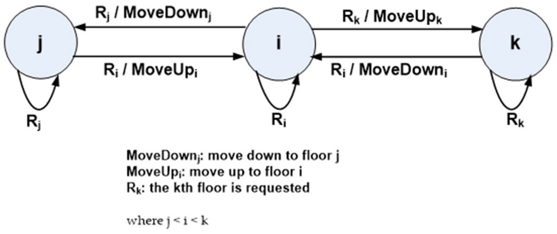
Our elevator system, denoted as A1, encompasses a finite set of states, specifically Nf states, each symbolizing the elevator’s present floor. All states within this automaton are designated as accepting states, with the initial state correspondingly set to f0. Within the context of each state or floor, the up and down actions facilitate transitions that align with the positional relationship between the current floor and the destination floor. Notably, these actions are constrained by specific rules, disallowing transitions that are incompatible with the relative positions of the current and prospective floors.
Figure 1 provides a visual representation of the resultant automaton.
With these elements in place, a classical planner can solve this problem and find a sequence of actions that will transport all passengers to their desired floors while minimizing the cost of the actions taken.
Single-agent classical planning task tuple π = {A, F, I, G} for an elevator system:
- (a)
A: The set of possible actions that the elevator can take, which includes moving up, moving down, stopping, loading passengers, and unloading passengers.
Move up: the elevator moves up one floor.
Move down: the elevator moves down one floor.
Stop: the elevator stops at the current floor.
Load: the elevator picks up a passenger at the current floor.
Unload: the elevator drops off a passenger at the current floor.
More details of each action in the elevator system and their preconditions and effects can be found in
Table 1.
Constraints: The elevator cannot carry more passengers than its capacity, and passengers can only be dropped off at their desired floor.
The operation of an elevator must follow five essential constraints as outlined by Closs in 1970 [
19]. These constraints are as follows:
An elevator is not allowed to stop at a floor if no passenger is entering or exiting the elevator;
An elevator cannot bypass a floor where a passenger wishes to disembark;
A passenger is not allowed to enter an elevator that is moving in the opposite direction to where they need to go;
Once a passenger is in the elevator, it cannot change direction of travel;
Car calls always take priority over floor calls.
- (b)
F: The set of possible states in the elevator system, which includes the location of the elevator, the passengers in the elevator, and the passengers waiting at each floor.
A finite-state transition model is a mathematical representation of the behavior of a system. It is composed of a set of states, transitions between those states, and actions associated with each transition. To be more generic, we introduce the following, as shown in
Figure 1.
The input set, denoted as Is = {Rj, 1 ≤ j ≤ Nf}, represents the floors that have been requested; for example, Rj indicates that the jth floor has been requested. The output set, denoted as Os = {MoveDowni, MoveUpk}, represents the direction and the number of floors that the elevator should move, for example, MoveDowni means that the elevator should move down i floors, and MoveUpk means that it should move up k floors.
The set of states, denoted as S = {S
i, 1 ≤ i ≤ Nf}, represents the floor that the elevator is currently on. For instance, in
Figure 1, if the current floor is S
i and there is a request for the jth floor (R
j), the elevator will move down (MoveDown
j) to floor j, changing from state S
i to S
j.
- (c)
I: The initial state of the system, which includes the location of the elevator at floor 1, all passengers waiting on different floors, and the elevator being empty.
- (d)
G: The goal state of the system, which includes all passengers being transported to their desired floors.
Cost Function: The cost of each action.
With these elements in place, a classical planner can use a search algorithm to find a sequence of actions that will take the system from the initial state to the goal state while minimizing the cost of the actions taken. For the evaluation of the cost function, we employ two distinct methodologies. The first method, called the heuristic solution, relies on employing two straightforward heuristics outlined in
Section 3. Subsequently, we use the optimal solution approach, detailed in
Section 4; this approach involves the utilization of the genetic algorithm and simulated annealing algorithm for optimization.
3. Heuristic Solution Applied to an Elevator Group Control System
The elevators are limited in terms of their available actions. When the elevator is on a floor, it has the option to move either up or down. If it is between floors, it must either stop at the next floor or continue past it. However, due to passenger expectations, there are certain limitations on these actions. For example, the elevator cannot bypass a floor if a passenger wants to disembark, and the elevator cannot change direction until it has fulfilled all the requests in its current direction. In addition, there are three additional guidelines that have been incorporated to reflect basic prior knowledge. The elevator cannot stop at a floor unless someone wishes to enter or leave, it cannot stop to pick up passengers if another elevator is already stopped at that floor, and it should give priority to moving up rather than down. Given these limitations, the only available choices for each elevator are to stop or to continue.
To evaluate the cost of a plan
π, we can use the following formula:
where
means to sum up the cost of each action in the plan π and
c(
ai) is the cost of each individual action.
Heuristic 1: Car calls are typically addressed through a conventional mechanism involving a reversal process at either the highest floor attained or the lowest floor encountered. Consequently, the elevator responds to both its internal car calls and external landing calls in a sequential manner based on the floor sequence relative to its current position and the committed direction of travel.
Heuristic 1 suggests a strategy for the management of elevator calls, adhering to the principles of directional distributive control. In this approach, landing calls are processed in a conventional manner, involving a reversal of direction when the elevator reaches the highest downward call or the lowest upward call. Consequently, the elevator responds to both car and landing calls in accordance with the sequential order of floors, commencing from its current location and adhering to the direction of travel that aligns with its ongoing commitment.
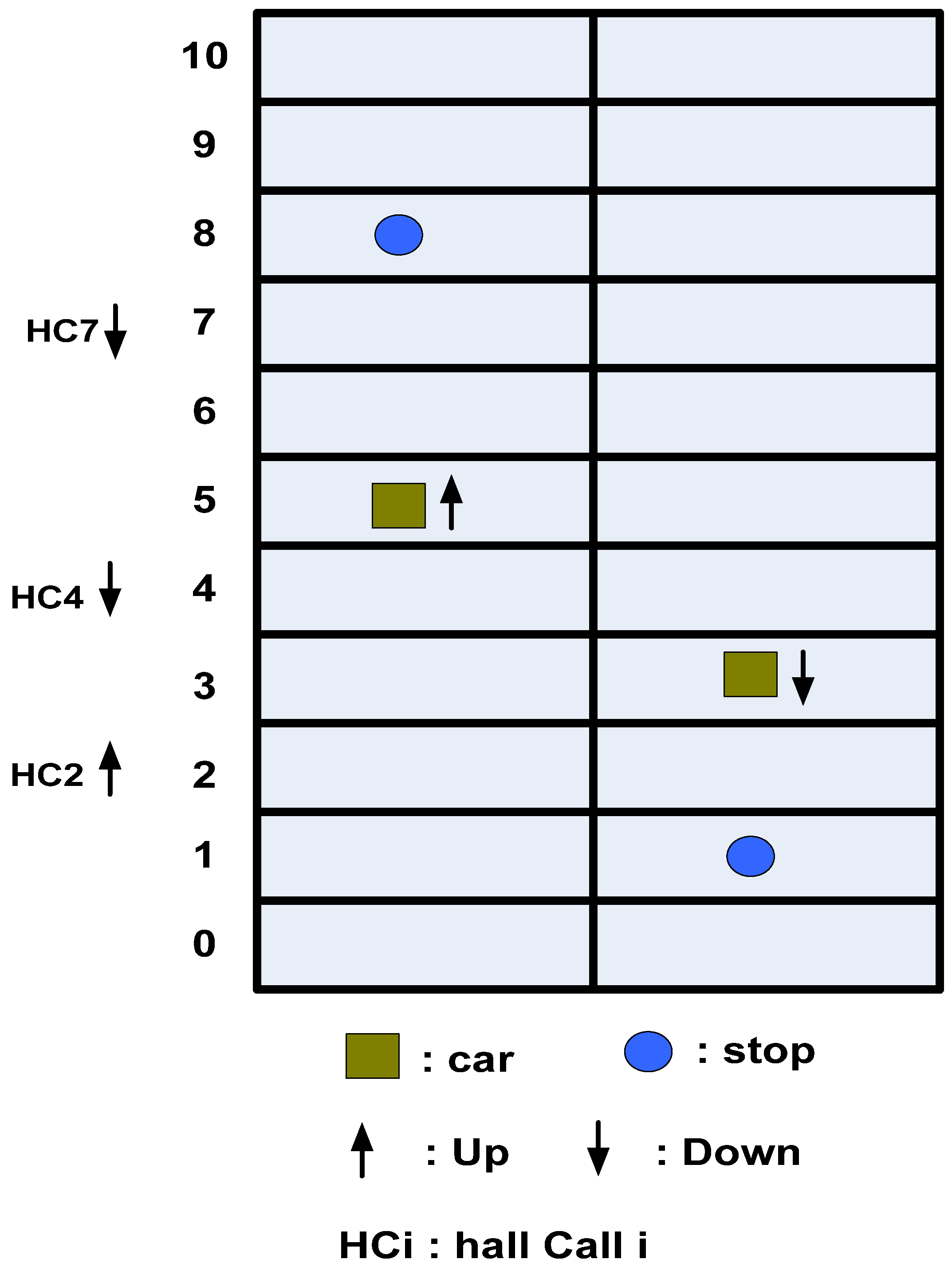
Suppose we have an elevator system with two cars and eleven floors. Car 1 is currently on floor 5, and car 2 is currently on floor 3. Car 1 wants to move up to floor 8, and car 2 wants to move down to floor 2 (see
Figure 2).
The time needed to stop is equal to 4 units of time. The time to go from one floor to a successive one is equal to 3 units of time. The time needed to change direction is equal to 1 unit of time (one unit of time is equivalent to one second).
Car 1: moves up from floor 5 to floor 8 (9 units of time), stops at floor 8 (4 units of time), moves up from floor 8 to floor 10 (6 units of time), changes direction (1 unit of time), moves down from floor 10 to floor 7 (9 units of time), stops at floor 7 (4 units of time), moves down from floor 7 to floor 4 (9 units of time), stops at floor 4 (4 units of time), moves down from floor 4 to floor 0 (12 units of time), changes direction (1 unit of time), moves up to floor 2 (6 units of time).
Car 2: moves down from floor 3 to floor 1 (6 units of time), stops at floor 1 (4 units of time), moves down from floor 1 to floor 0 (3 units of time), changes direction (1 unit of time), moves up from floor 0 to floor 2 (6 units of time), stops at floor 2 (4 units of time), moves up from floor 2 to floor 10 (24 units of time), changes direction (1 unit of time), moves down from floor 10 to floor 7 (9 units of time), stops at floor 7 (4 units of time), moves down from floor 7 to floor 4 (9 units of time).
Table 2 shows the cost of a trip between the actual position of cars (Car 1 and Car 2) and hall calls (HC2, HC4, HC7) based on the first heuristic.
Car 1 can perform the following calls: HC7 and HC4 (arriving at HC4 at 42 units of time).
Car 2 can perform the following call: HC2 (arriving at HC2 at 20 units of time).
Heuristic 2: Priority is given to the set of calls in the same direction (without reversing direction), or the direction of the car is changed when all calls in the same direction are responded to, beginning from the highest position if the direction is DOWN or from the lowest position if the direction is UP (in case of equity of opposite directions, priority is given to the same direction).
Suppose we have an elevator system with two cars and eleven floors. Car 1 is currently on floor 5, and car 2 is currently on floor 3. Car 1 wants to move up to floor 8, and car 2 wants to move down to floor 2 (see
Figure 2).
The time needed to stop is equal to 4. The time to go from one floor to a successive one is equal to 3. The time needed to change direction is equal to 1.
Car 1: moves up from floor 5 to floor 8 (9 units of time), stops at floor 8 (4 units of time), changes direction (1 unit of time), moves down from floor 8 to floor 7 (3 units of time), stops at floor 7 (4 units of time), moves down from floor 7 to floor 4 (9 units of time), stops at floor 4 (4 units of time), moves down from floor 4 to floor 2 (6 units of time).
Car 2: moves down from floor 3 to floor 1 (6 units of time), stops at floor 1 (4 units of time), changes direction (1 unit of time), moves up from floor 1 to floor 2 (3 units of time), stops at floor 2 (4 units of time), moves up from floor 2 to floor 7 (15 units of time), stops at floor 7 (4 units of time), changes direction (1 unit of time), moves down from floor 7 to floor 4 (9 units of time).
Table 3 shows the cost of a trip between the actual position of cars (Car 1 and Car 2) and hall calls (HC2, HC4, HC7) based on the second heuristic.
Car 1 can perform the following calls: HC7 and HC4 (arriving at HC4 at 30 units of time).
Car 2 can perform the following call: HC2 (arriving at HC2 at 14 units of time).
A waiting time longer than 30 s is usually considered long and undesirable for this service [
20]. That is why we need to study this problem with a genetic algorithm and simulated annealing to reduce the average waiting time.
4. Optimal Solution Applied to an Elevator Group Control System
Each car within the elevator group is associated with a unique array, characterized by the upward and downward calls to each floor for the car. Therefore, the length of each solution is (2 × N), where N represents the total number of floors in the structure.
For individual cars, the solution represents the allocation of up and down hall calls, as outlined in
Table 4 and
Table 5. The example tables correspond to a 10-floor architectural configuration. The solution uses binary encoding, where ‘0’ denotes the absence of hall-call allocation for the respective car, while ‘1’ signifies the assignment of the registered hall call on that floor to the designated car.
Table 6 presents upward and downward hall calls for the whole elevator group.
All possible solutions that are encoded as stated above are evaluated to determine the quality (or fitness) of such solutions.
The fitness estimation procedure relies on the state of the elevator (stationary, ascending, or descending) and is based on four peak values denoted as X1, X2, X3, and X4.
For case (i), where the elevator is stationary or ascending:
- -
X1 represents the current floor;
- -
X2 signifies the highest floor for passengers going up;
- -
X3 denotes the lowest floor for passengers going down;
- -
X4 represents the highest floor lower than X1 for passengers going up, where X4 < X1.
Equation (1) considers the maximum known upward trip, the maximum known downward trip, and the subsequent maximum known unexecuted upward trip in the initial upward traffic, given X4 < X1. Notably, the mathematical expression excludes passenger destination trips, as their information is unknown until passengers enter the cabin.
For case (ii), where the elevator is descending:
- -
X1 represents the current floor;
- -
X2 signifies the lowest floor for passengers going down;
- -
X3 denotes the highest floor for passengers going up;
- -
X4 represents the lowest floor higher than X1 for passengers going down, where X4 > X1.
Equation (2) considers the maximum known downward trip, the maximum known upward trip, and the subsequent maximum known unexecuted downward trip in the initial downward traffic, given X4 > X1.
Then, the average value is calculated as (3):
where
n is the number of cars in the group.
We consider a given group of two cars in a 10-story building. Calls to the upper and lower halls are assigned as shown in
Table 6. Let us suppose that the value for estimated interfloor trip time = 3.
Car 1 is moving down, and it is on floor 3.
The fitness of the first car is calculated using Equation (2), where:
- -
X1 = 3 represents the current floor;
- -
X2 = 1 signifies the lowest floor for passengers going down;
- -
X3 = 7 denotes the highest floor for passengers going up;
- -
X4 = 4 represents the lowest floor higher than X1 for passengers going down, where X4 > X1.
The fitness is then calculated as:
Car 2 is moving up, and it is on floor 3.
The fitness of the second car is calculated using Equation (1), where:
- -
X1 = 3 represents the current floor;
- -
X2 = 10 signifies the highest floor for passengers going up;
- -
X3 = 2 denotes the lowest floor for passengers going down;
- -
X4 = 2 represents the highest floor lower than X1.
The fitness is then calculated as:
The final fitness is thus given by Equation (3):
The evaluation of the quality of the solution is carried out according to the procedure mentioned above for each possible encoded solution. This assessment has a significant impact on the search trajectory in the feasibility region dictated by the SA algorithm or on the potential success of the offspring of the GA.
4.1. Simulated Annealing Algorithm
Simulated annealing is a famous iterative metaheuristic [
21]. To obtain an approximate solution (close to the optimum) for computational optimization problems, the SA method based on only the point search technique has been commonly favored by experts as well as researchers. SA begins with the initial solution and tries to improve it in time by producing modifications to that solution at every step. The principal characteristic of SA is that obtaining a worse solution can be accepted with some likelihood that changes in time depending on the temperature and the adjustment of the solution. Consequently, while looking for the best solution to a given problem, the value of every candidate solution should be assessed, and this is accomplished by utilizing an objective function.
The algorithm of SA is presented in the following Algorithm 1.
| Algorithm 1 Simulated Annealing |
begin
1 Input: Solinitial; Tinitial; Tmin; reduction factor α
2 Output: Solbest
3 Current ← Solinitial; Optimal ← Current; T ← Tinitial
4 while (T > Tmin) do
5 for i = 0 to N (maxIter)
6 Next ← a randomly selected successor of Current
7 if fitness (Next) < fitness (Current) then
8 Current ← Next
9 if fitness (Next) < fitness (Optimal) then
10 Optimal ← Next
11 Topt ← T
12 end if
13 else
14 ∆fitness = fitness (Next) − fitness (Current)
15 r ← random (0, 1)
16 if r < exp (-∆fitness/kT) then
17 Current ← Next //Current = Next only with probability exp(−∆E/KT)
18 end if
19 end if
20 end for
21 T ← α x T
22 end while
end. |
The local search is executed N times (maximum of iterations); after that, the temperature T is decreased as in T ← αT, where the parameter α is considered as the reduction factor (0 ≤ α ≤ 1).
In the SA algorithm, it is essential to obtain precise values for three parameters: the initial temperature (T), the reduction factor (α), and the maximum number of iterations permitted for each temperature value (N). These parameters are obtained as a product of calibration tests. The calibration process of simulated annealing is as follows:
- (1)
The initial temperature T is considered in the range between 10 and 180;
- (2)
The reduction factor is tested at the range between 0.1 and 1;
- (3)
The maximum number of iterations N is verified in the range between 1 and 18.
Significant research efforts have been made to identify optimal parameters for the SA algorithm [
22]. However, it was proven that an optimal and universally applicable configuration does not exist. In fact, various problems require particular parameters specific to each. If each algorithm parameter is conceptualized as a variable and SA performance is conceptualized as an objective value, the search for the best parameter settings is equivalent to navigating this landscape to find the global optimum, a task that varies from problem to problem and involves identifying the most favorable configuration in this broad and diverse parameter space. In establishing parameter values for SA, a common approach involves parameter tuning, relying on systematic experimentation of different parameter values. This method involves conducting multiple tests to determine the values that produce optimal results and then adopting these selected values for the final execution of the algorithm. Importantly, this parameterization technique complies with a fixed value paradigm during algorithm execution, where the selected values remain constant, without dynamic change during runtime.
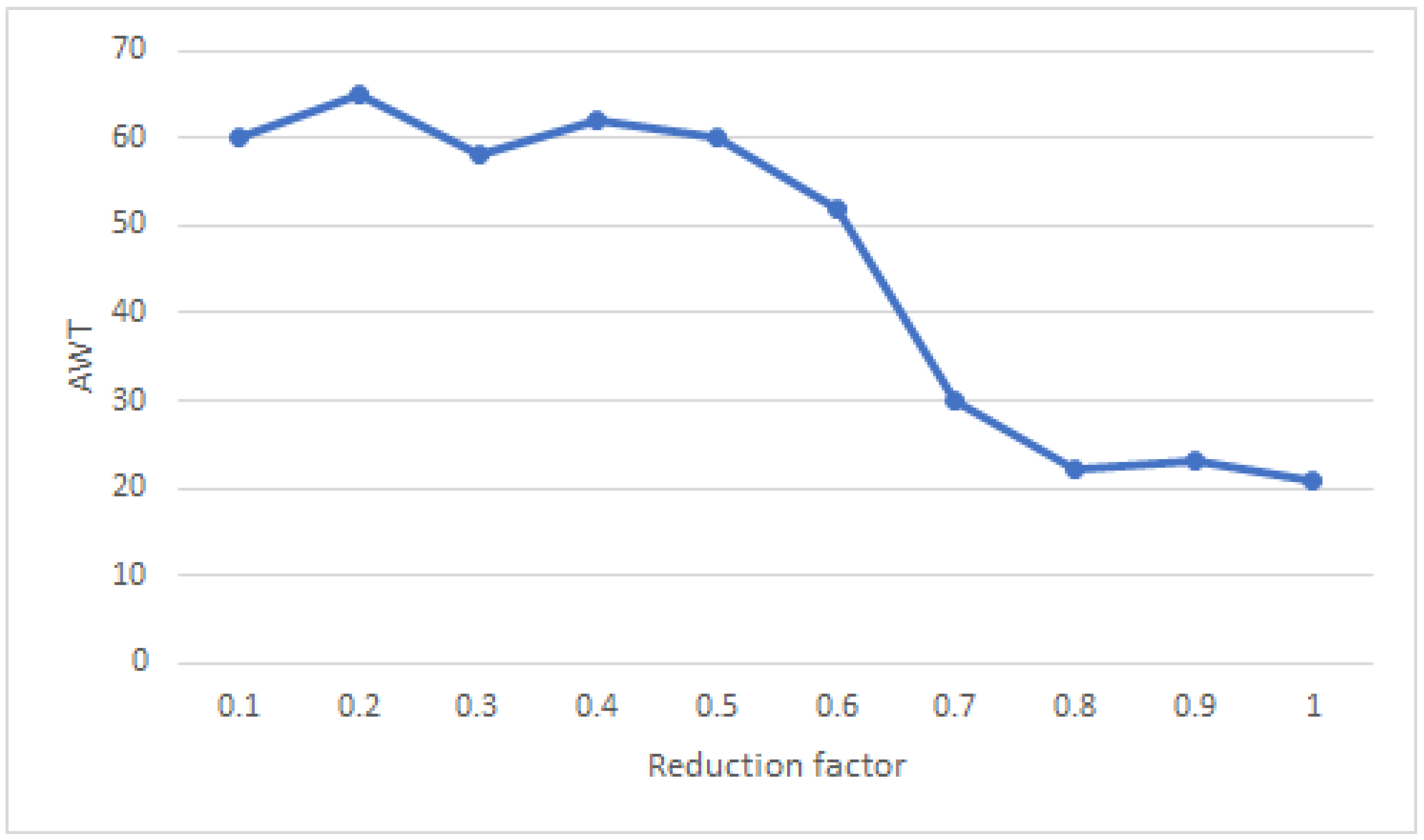
Figure 3 demonstrates that choosing the reduction factor (α) is of supreme significance. A reduction factor that is too small (from 0.1 to 0.6) will lead to a very bad solution (the average waiting time is very high), whereas a larger value will cause the average waiting time to continue oscillating around the global minimum. This can be explained by the fact that when the reduction factor (α) is reduced, the number of iterations is therefore limited, but if the reduction factor (α) is elevated, the number of iterations is consequently very high. Therefore, it is more feasible to find the global minimum with a high reduction factor (α) value.
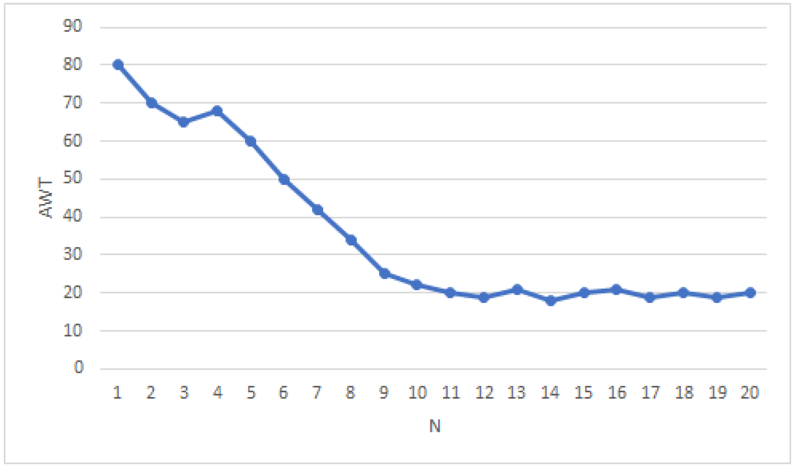
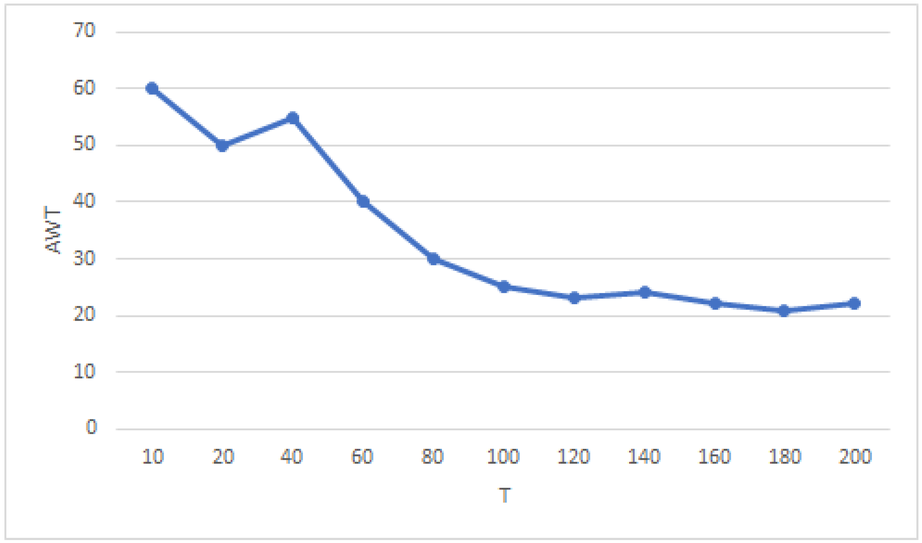
Figure 4 shows that the N value is very important in the SA. A smaller value (between 1 and 7) will cause a faster convergence to a local minimum, taking less time, whereas a higher value will cause a slower convergence to a global minimum, taking more time. This can be justified because when the N value is reduced, the number of repetitions for the same temperature value is limited, but if its value is too high, then the number of repetitions for the same temperature value will be high. That explains why the probability of finding the best solution is ensured with a high value of N.
Figure 5 demonstrates that the initial value of temperature T is very important for obtaining good results with the simulated annealing algorithm. If the initial value is small (from 0 to 50), the simulated annealing research may have poorer performance that it converges to a bad solution (not the global optimum). However, if the initial value is great, then it is more likely to converge to the best solution, which means the global optimum. This can be explained as follows: when the temperature T is reduced, the probability of accepting a bad move tends toward zero, and so the algorithm converges to the local minimum. However, when the temperature T is high, the SA sometimes accepts a bad move to escape the local optimum.
4.2. Genetic Algorithm
The genetic algorithm is an evolutionary method utilized to determine a heuristic global optimum [
23]. Its heuristic is based on Charles Darwin’s evolution hypothesis, with a deterministic process to select individuals, where the fitter individuals are more likely to survive and to replicate, and a stochastic process related to random individual mutation and crossover. Therefore, the GA globally converges to the optimal solution. Algorithm 2 presents the pseudocode of the genetic algorithm.
| Algorithm 2 Genetic algorithm |
begin
generate initial population
compute the fitness of each individual
while NOT finished DO
/* produce new generation */
for population_size
Evaluate each individual based on the fitness function
/* crossover phase */
select two individuals from the old generation for reproducing based on the fitness function
recombine the two individuals to give two descendants
insert these two descendants in the new generation
/* mutation phase */
select individuals based on their fitness function to do mutation
insert altered individuals in a new generation
end for
if population has converged THEN
finished: = TRUE
end if
end. |
The parameters of GA are also obtained by the same approach. Three important parameters need to be calibrated; these parameters are as follows: (1) the mutation rate in the range [0, 0.9], (2) the population size in the range [2, 140], and (3) the number of repetitions N in the range [10, 200].
The effectiveness of genetic algorithms (GAs) depends on the careful selection of their basic parameters, i.e., population size, mutation rate, and number of generations, which interact in a complex way collectively. To verify GA performance based on these parameters, extensive research has been undertaken. Knowing the complex interdependence of these parameters directly affects solution quality, and maintaining a balanced configuration of parameter values increases GA’s solution search effectiveness [
24]. The three basic parameters used by GA are as follows:
Mutation rate (probability): Dictating the frequency of chromosome mutations throughout a generation, the mutation rate is in the range of [0, 1]. Its role is crucial to prevent local optimization, but an excessively high mutation rate can lead GA toward random search rather than directed optimization.
Population size: This parameter directly affects the size of the search space when entered into the algorithm. A smaller population can limit exploration, resulting in a potential trap of local optimization, while an overly large population increases computational requirements without increasing the quality of the solution.
Number of generations: Termination is set to occur after a specified number of cycles; the appropriate value of this parameter varies depending on the nature and complexity of the problem. Its relevance can fluctuate depending on the design of the GA, especially when termination is based on specific criteria rather than a predetermined number of generations.
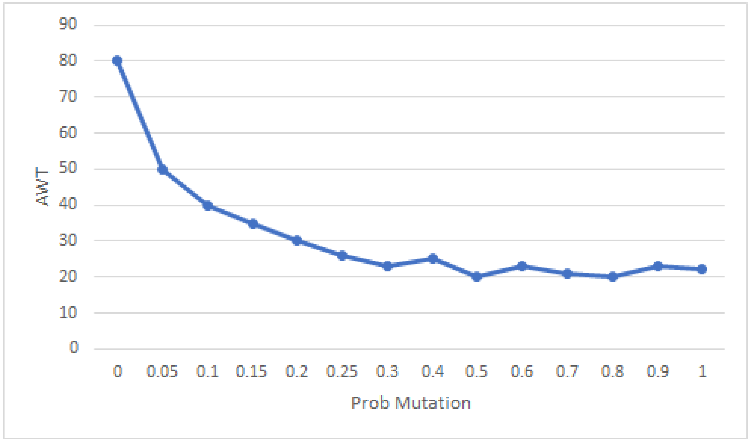
Figure 6 shows that choosing the mutation probability is very important. A smaller value (between 0 and 0.1) leads to a bad solution in terms of the fitness value. Whereas a higher value will cause fitness to continue oscillating near the global minimum. This can be justified as follows: when the mutation probability is reduced, the GA converges quickly to a local minimum without having the chance to discover new solution candidates, but if the mutation probability is high, the GA converges to a global minimum with better coverage of different solution candidates.
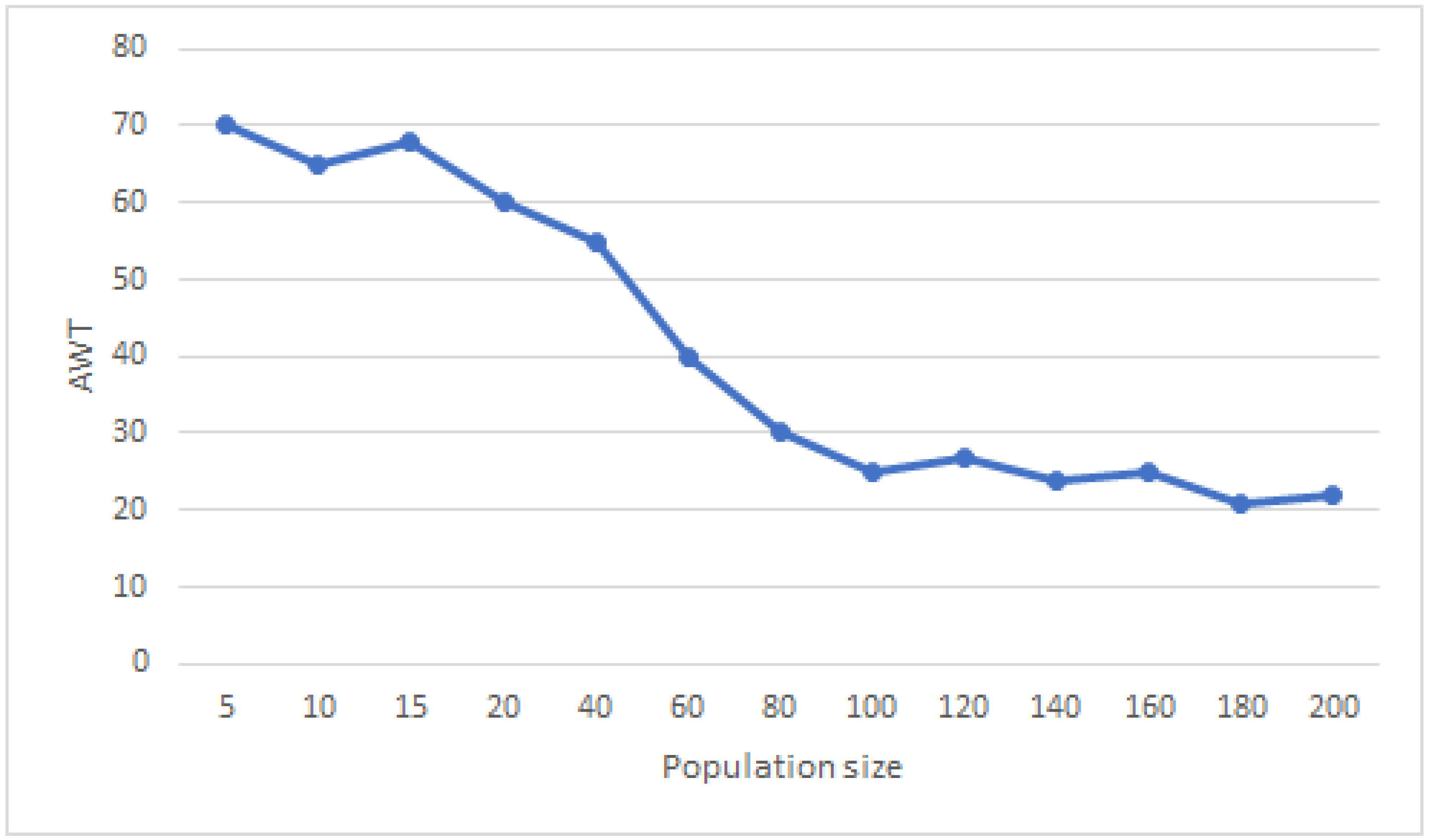
Figure 7 demonstrates that the population size is of supreme significance. A smaller value (from 1 to 40) will cause the algorithm to converge quickly to a local minimum, whereas a larger value will cause the algorithm to converge slowly to a global minimum. This can be justified as follows: when the N value is reduced, the number of repetitions for the same temperature value is limited, but if the value is too high, then the number of repetitions for the same temperature value will be high. That explains the probability of finding the best solution.
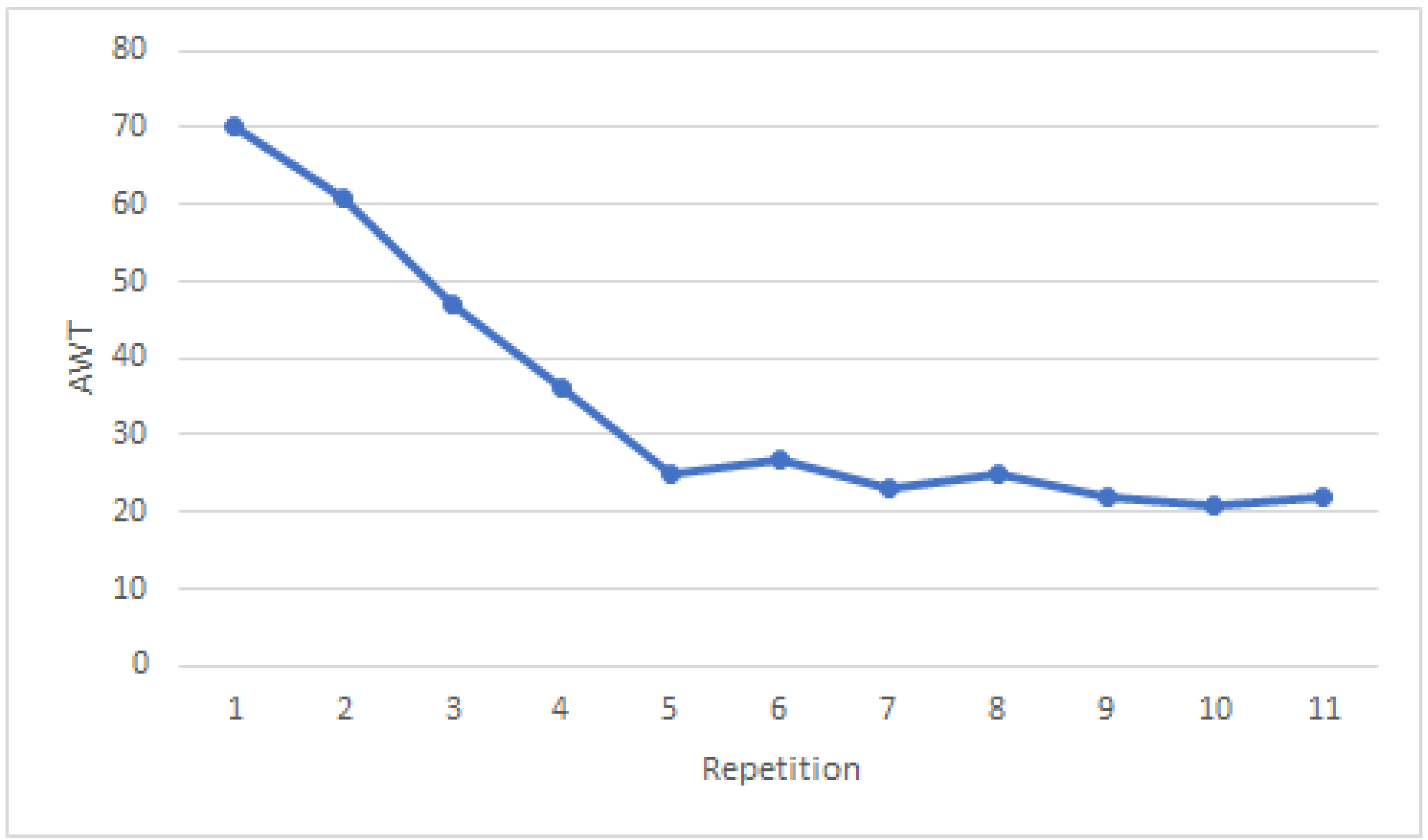
Figure 8 shows that the repetition value is an important parameter for GA. Whenever the value is too small (from 10 to 40), the genetic algorithm is considered to have lower performance, converging to a bad solution. However, if the value is too high, then it takes more time to converge but is more likely to converge to the best solution, which means the global optimum. This can be explained by the fact the higher the repetition value, the more likely the algorithm is to find the global minimum.


