Article

Research on the Remaining Life Prediction Method of Rolling Bearings Based on Multi-Feature Fusion

1
College of Electrical and Information Engineering, Lanzhou University of Technology, Lanzhou 730050, China
2
Key Laboratory of Gansu Advanced Control for Industrial Processes, Lanzhou 730050, China
3
National Demonstration Center for Experimental Electrical and Control Engineering Education, Lanzhou University of Technology, Lanzhou 730050, China
*
Author to whom correspondence should be addressed.
Appl. Sci. 2024, 14(3), 1294; https://doi.org/10.3390/app14031294
Submission received: 2 January 2024 / Revised: 30 January 2024 / Accepted: 31 January 2024 / Published: 4 February 2024
(This article belongs to the Special Issue Recent Advances and Innovation in Prognostics and Health Management)

Abstract

:
Rolling bearings are one of the most important and indispensable components of a mechanical system, and an accurate prediction of their remaining life is essential to ensuring the reliable operation of a mechanical system. In order to effectively utilize the large amount of data collected simultaneously by multiple sensors during equipment monitoring and to solve the problem that global feature information cannot be fully extracted during the feature extraction process, this research presents a technique for forecasting the remaining lifespan of rolling bearings by integrating many features. Firstly, a parallel multi-branch feature learning network is constructed using TCN, LSTM, and Transformer, and a parallel multi-scale attention mechanism is designed to capture both local and global dependencies, enabling adaptive weighted fusing of output features from the three feature extractors. Secondly, the shallow features obtained by the parallel feature extractor are residually connected with the deep features through the attention mechanism to improve the efficiency of utilizing the information of the front and back features. Ultimately, the combined characteristics produce the forecasted findings for the RUL of the bearing using the fully connected layer, and RUL prediction studies were performed with the PHM 2012 bearing dataset and the XJTU-SY bearing accelerated life test dataset, and the experimental results demonstrate that the suggested method can effectively forecast the RUL of various types of bearings with reduced prediction errors.

1. Introduction

With the continuous development of the industrial level, the metallurgical industry plays an important role in the process of achieving comprehensive industrialization in China, which is of great significance to the industrial and economic development of the country [1]. In the metallurgical beneficiation process, the grinding link in mechanical equipment is crucial [2]. However, as metallurgical equipment works in harsh environments all year round, the longer the equipment is used, the more difficult it is to avoid wear, aging, and failure of rolling bearings [3,4,5]. Such wear and failure will not only affect economic production efficiency but may also c ause accidents in serious cases, resulting in casualties and property losses. Therefore, the prediction of the remaining useful life (RUL) of rolling bearings is a meaningful and extremely important work [6].
In the past few years, many scholars have devoted themselves to the research of bearing RUL prediction methods. These methods can be broadly categorized into two primary groups: model-driven and data-driven approaches. Model-driven-based methods achieve bearing RUL prediction by constructing a physical or mathematical model that can accurately describe the bearing degradation process, which mainly include Kalman filtering [7], particle filtering [8], Wiener’s process [9], Gamma process [10], and Weibull distribution [11] methods. The construction process requires not only the parameters of the actual engineering system obtained after a series of measurements but also a great deal of a priori knowledge. While model-based approaches are useful in predicting the general trend of mechanical degradation, it is difficult to accurately simulate the degradation trend with simple physical or mathematical models in practical industrial applications, especially for complex mechanical equipment. Due to the swift advancement of intelligent sensing and machine learning technologies, a substantial quantity of condition monitoring data is gathered in industrial production, leading to the quick growth and increased viability of the data-driven approach.
Currently, machine learning and deep learning are the main research directions for data-driven methods [12]. In traditional machine learning approaches to unstructured data, such as text, images, or audio, a process of feature engineering is often required to transform the raw data into features with interpretable and representational capabilities. This process requires domain expertise and experience to select and design appropriate feature extraction methods. Deep learning has the ability to learn features with representational power directly from raw data through the learning capabilities of multi-layer neural networks. Compared to traditional methods, deep learning models possess the ability to autonomously extract and acquire abstract features of a higher level from unstructured data, eliminating the need for manual feature creation and selection. Therefore, with sufficient data, deep learning prediction methods are more effective than traditional machine learning and are now widely used in the domain of RUL forecasting [13].
Since Hinton et al. [14] proposed the deep learning theory, Recurrent Neural Network (RNN), Convolutional Neural Network (CNN), and their derivative networks have gained wide application in the field of lifetime prediction. For example, Guo et al. [15] introduced a health indicator (RNN-HI) based on RNN to forecast the RUL of bearings. Catelani et al. [16] combined an RNN-based estimation method with a filter-based state-space estimation technique to enhance the accuracy and precision of the RUL prediction for lithium-ion batteries. However, RNNs may suffer from gradient explosion during model training, so researchers have made many improvements to the RNN structure to solve the problem and have obtained many improved models. Among them, the Long Short-Term Memory (LSTM) model, introduced by Hochreiter and Schmidhuber [17], is widely recognized as the most prominent in its field. Miao et al. [18] employed LSTM to construct a dual-task deep LSTM model for simultaneously learning the assessment of aero-engine degradation and predicting its RUL. Although LSTMs are capable of capturing temporal dependencies in time-series data both before and after a given point, their intricate chain structure results in longer training periods and less sensitivity to extended time series. To enhance the effectiveness of prediction models, certain researchers have endeavored to implement RUL prediction with CNN. Ren et al. [19] developed a model based on deep CNN and LSTM for mining deeper information from limited data to accurately predict the remaining lifetime of lithium-ion batteries. Although CNNs provide a remarkable capability to extract features that are locally relevant, they lack sensitivity to temporal information and are prone to ignoring the back-and-forth correlation of temporal information in the data. In order to tackle this issue, Bai et al. [20] proposed a solution to address this problem by introducing a Temporal Convolutional Network (TCN) that integrates causal convolution with null convolution. This network exhibits similar temporal feature extraction capabilities as RNN and has shown promising results in time series modeling applications. Wang et al. [21] developed a TCN network that incorporates a soft threshold and attention mechanism to effectively capture important features and accurately forecast the RUL of mechanical devices. However, the convolution operation used in TCN, i.e., the extraction of local information, exhibits a deficiency in considering worldwide data and does not adequately account for relationships that span over a significant period of time in the sequence. In order to consider global correlations, some researchers have used Transformer to predict bearing RUL. Mo et al. [22] used the Transformer encoder as the backbone of the model to capture short-term and long-term dependencies and global feature representations in the time series, which in turn predicts their remaining lifespan.
In addition, in recent years, as smart manufacturing systems have improved, modern industries have increasingly implemented a significant number of signal sensors [23]. According to Li et al. [24], the use of many sensors in the industrial production process can result in the collection of a significant volume of data. This, in turn, can enhance the dependability of the health monitoring system for industrial equipment, so the information derived from multiple sensors is more valuable to study than the single sensor data. However, how to effectively utilize multi-sensor data and achieve fusion of feature information is still an open question.
To summarize, while deep learning techniques have shown promising outcomes in predicting the RUL of bearings, there are still unresolved concerns that require attention:
(1)
Most of the current research focuses on the utilization of single-sensor data, while insufficient attention is paid to the efficient integration and utilization of data from several sensors. Meanwhile, when using parallel networks for feature extraction, the same network structure is often adopted without giving full play to the advantages of multiple networks.
(2)
In most of the parallel attention mechanism structure research, each branch of the network utilizes the multi-head self-attention mechanism to adjust the internal connections inside the data. However, using the same feature extraction method to fuse the outputs of each branch network may result in important features being masked while redundant features are retained, ultimately affecting the overall performance of the network.
In order to tackle the aforementioned issues, this research presents a method for predicting the RUL of rolling bearings by utilizing a fusion of many features. Firstly, the multi-sensor data is normalized, and the sensor data is combined in each channel to produce an optimal fusion of data from several sensors; Then, a parallel multi-branch feature learning network was constructed using TCN, LSTM, and Transformer, where TCN analyzes the data to identify and extract the long-time series features, LSTM captures the time-correlated features in the series data, and Transformer extracts the global feature representation of the bearing data. Meanwhile, a parallel multi-scale attention mechanism that captures both local and global dependencies is designed to go a step further in capturing the global and local contextual information of the sequence in order to accomplish adaptive weighted fusion from the output features of the three feature extractors. Secondly, the shallow features obtained by the parallel feature extractor are residually connected to the deeper features through the attention mechanism in order to enhance the efficiency of utilizing the information from the before and after features. Finally, the fused features output RUL predictions through the fully connected layer. The predictive model allows for a more comprehensive description of the operating condition of ball mill rolling bearings by fusing multiple features multiple times and capturing factors that may have an impact on their remaining life. This improves the accuracy of the prediction model and more accurately forecasts the RUL of rolling bearings. This paper’s contribution can be summarized as follows:
(1)
By fusing information from multiple sensors, more comprehensive, accurate, and reliable information is obtained, and feature extraction by parallel processing TCN, LSTM, and Transformer gives full play to their respective advantages to enhance the efficiency of the prediction model and the precision of the forecast outcomes.
(2)
A parallel, multi-scale attention mechanism is designed. By fusing features in both the time and frequency domains, we are able to capture comprehensive and specific contextual information from sequential data while capturing local and global dependencies. A more comprehensive representation of the data can be achieved.
(3)
A multi-feature fusion model for predicting the RUL of rolling bearings is proposed, which can enhance valuable information while reducing redundant information, ultimately achieving the effective fusion of multiple features. Better prediction results than the current prediction methods are achieved in the experimental validation.
The subsequent sections of the paper are structured in the following manner: Section 2 provides a concise overview of the relevant background information; Section 3 provides a comprehensive explanation of the proposed methodology; Section 4 demonstrates the efficacy of the proposed method by analyzing two bearing datasets; and Section 5 provides the conclusion.

2. Theoretical Background

2.1. Temporal Convolutional Network

The combined process of one-dimensional full convolution, causal convolution, and dilation convolution is represented by dilation causal convolution, as shown in Figure 1. In Figure 1, the input sequence is denoted as X = { x 1 , x 2 , , x t 1 , x t } . The output sequence, denoted as Y = { y 1 , y 2 , , y t 1 , y t } , is obtained by performing a one-dimensional dilated causal convolution operation with a convolution kernel size of 3 on a three-layer input sequence, which is the same as the input sequence. The dilation factor, denoted as d N , is often set to 2 in convolution calculations.
The sensory field v is determined by the dimensions of the convolution kernel, the number of layers of the convolution computation, and the dilation factor, which is calculated as follows:
v = 1 + i = 0 l 1 ( k 1 ) b i
where k , l , and b represent the size of the convolutional kernel, the number of convolutional layers in the network, and the base of the expansion factor, respectively. which is usually set to b = 2.
For the task of TCN, we are provided with a one-dimensional input sequence x n and a convolution kernel f : { 0 , 1 , , k 1 } . The dilated causal full convolution at the position of the sequence s is computed as follows:
F ( s ) = i = 0 k 1 f ( i ) x s d i
where x s d i is the ( s d i ) t h element in the preceding layer, and f ( i ) is a convolution kernel function that maps an index i to a real weight. x s d i denotes the ( s d i ) t h element of the input sequence x after it has been adjusted by the expansion causality operation, and the remaining parameters retain their former significance.
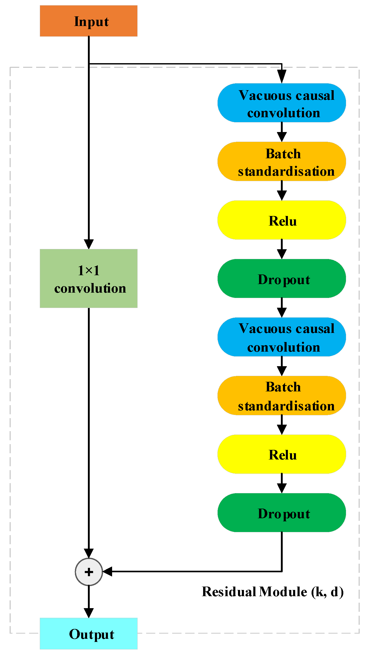
Furthermore, TCN employs residual block connectivity to enhance the depth of the network, which can effectively weaken the gradient problem and further increase the model sensory field by connecting multiple residual blocks together. The structure of each residual block is depicted in Figure 2.

2.2. Long Short-Term Memory

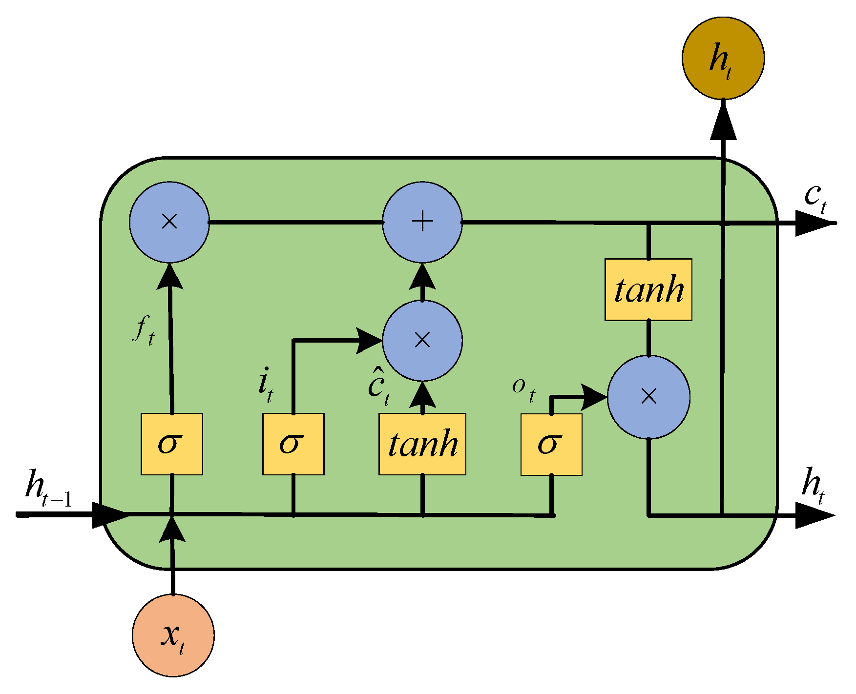
RNN is a specialized model for processing time-series data by introducing the concept of “time”, in which information from a past period of time can be remembered. LSTM is a special structure proposed to overcome the gradient explosion or vanishing problem of RNN, which possesses the ability to retain information over an extended duration and can extract information not only from a single data point but also from an entire data series [17]. LSTM is mainly divided into three gates, namely, the oblivion gate, the input gate, and the output gate, and the structure is seen in Figure 3.
The core concepts of LSTM lie in the cell state, which corresponds to the path of information transmission, and the gate structure, which enables the addition and removal of information, which is controlled using the S i g m o i d activation function. The input gate, denoted as i t , regulates the amount of information that should be stored for the candidate state, denoted as C ^ t , at the present time. The forgetting gate, denoted as f t , regulates the amount of information that should be discarded from the internal state, represented as C t 1 , from the previous time step. The output gate, denoted as o t , regulates the amount of information that is transmitted from the internal state, represented as C t , to the exterior state, denoted as h t , at the present time, and the formulae for the three gates are shown below:
i t = σ ( W i x t + U i h t 1 + b i )
f t = σ ( W f x t + U f h t 1 + b f )
o t = σ ( W o x t + U o h t 1 + b o )
C t = f t C t 1 + i t C ^ t
h t = o t tanh ( C t )
C ^ t = tanh ( W c x t + U c h t 1 + b C )
where x t represents the input feature, C t is the memory unit, C t 1 represents the memory unit of the previous moment, C ^ t represents the memory unit of the current state of the candidate, h t denotes the external state, and h t 1 denotes the external state of the preceding moment. W i , W f , W o , and W c denote the input weight vectors of the input gate, the forget gate, the output gate, and the candidate unit, respectively. U i , U f , U o , and U c denote the cyclic weight vectors of each gating unit, respectively. The activation function σ is the S i g m o i d , while the activation function tanh is the hyperbolic tangent. The symbol “ ” represents the vector product.

2.3. Enocder of Transformer

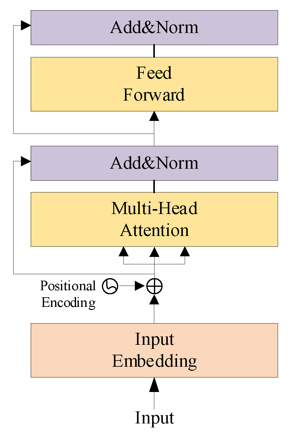
The Transformer encoder comprises two primary components: the multi-head attention mechanism and the feed-forward network. Each part is followed by connecting the residual network and the layer normalization module. The structure of the Transformer encoder is depicted in Figure 4.
Multiple attention mechanisms are stacking operations performed by multiple attention mechanisms to get the attention weight of each word in a sentence. The inputs to the attentional mechanism are three matrices of equal dimensions Q = [ q 1 , q 2 , , q n ] , K = [ k 1 , k 2 , , k n ] and V = [ v 1 , v 2 , , v n ] , where q i R d h , k i R d h , and v i R d h , d h denote the dimensions of the hidden layer. By querying the sequence Q , the sequence of keys K , and the sequence of values V , the attention value can be obtained as follows:
A ( Q , K , V ) = s o f t max ( Q K T d k ) V
where d k denotes the scaling factor, the main purpose of which is to prevent the gradient from disappearing during backpropagation.
The multi-head attention mechanism obtains feature vectors from different representation subspaces and then stitches and linearly transforms the results obtained from multiple attention heads:
h i = A ( W i Q Q , W i k K , W i V V )
M = C ( h 1 , , h h ) W O
where W i Q R d q × d h , W i K R d k × d h , W i V R d v × d h , and W i O R d o × d h are weight matrices.
The input vectors E s , E a , and E s a are subjected to residual network and normalization layer operations with Equation (11), which are calculated as follows, using E s as an example:
X s = L ( E s + M ( E s ) )
The feed-forward network converts the hidden layer representation acquired by the multi-head attention mechanism, which is computed assuming the input sequence is H as follows:
F ( H ) = max ( 0 , H W 1 + b 1 ) W 2 + b 2
where the weight matrix is denoted by W 1 and W 2 , whereas the bias values are denoted by b 1 and b 2 . Finally, the H s , H a , and H s a hidden layer representations are obtained by residual network and normalization layer computation. Taking the contextual hidden layer representation H s as an example, the computational formula is as follows:
H s = L ( X s + F ( X s ) )

3. Prediction of RUL Based on the Multi-Feature Fusion Method

The precise RUL of a bearing in real industrial production processes is uncertain at any particular point. Therefore, analyzing the historical operating data of existing bearings is crucial for industrial safety as it allows for an accurate projection of the lifespan of other bearings. To this end, a RUL prediction approach is proposed that utilizes multi-feature fusion, which consists of four main parts: multi-sensor data fusion processing, parallel TCN-LSTM-Transformer feature extractor construction, parallel multi-scale attention mechanism design, offline model training, and online bearing RUL prediction. The structure of the lifetime prediction network, which utilizes multi-feature fusion, is illustrated in Figure 5. Firstly, the multi-sensor data is normalized, and the sensor data is combined in each channel to produce an optimal fusion of data from several sensors; Secondly, a parallel multi-branch feature learning network was constructed using TCN, LSTM, and Transformer, where TCN extracts the local features of the data, LSTM captures the long-term dependencies present in the sequential data, and Transformer extracts the global feature representation of the bearing data. Meanwhile, a parallel multi-scale attention mechanism that captures both local and global dependencies is designed to go a step further in capturing the global and local contextual information of the sequence in order to accomplish adaptive weighted fusion of the output features from the three feature extractors. Next, the shallow features obtained by the parallel feature extractor are residually connected to the deeper features through the attention process, which enhances the efficiency of utilizing both the preceding and subsequent feature information. Finally, the fused features output RUL predictions through the fully connected layer.

3.1. Fusion of Multisensor Data

Data processing is a critical step in life prediction, and in order to eliminate, as much as possible, the reliance on expert knowledge in this part of the process, Multiple sensors provide the capability to gather vibration data from various positions on the bearing, in contrast to a single sensor, so that feature information from different viewpoints and locations can be obtained. By fusing these diverse characteristics, the condition of the bearing system may be described more comprehensively, providing a richer set of input features. Therefore, this paper employs a multi-sensor information fusion strategy to enhance the quantity of feature information included in the model inputs. The fusion process is illustrated in Figure 6.
Assuming the existence of M rolling bearings and their performance degradation data, the performance degradation data of C sensors will be gathered for each bearing, and each sensor will have the same sample period ( t ). Moreover, the t th data sample collected by the C th sensor may be represented as X t c , X t c H × 1 , where each sample’s length is represented by H, and each sensor’s data may be seen as a separate data channel. To lessen the impact of variations in the data distribution across several bearings, each sensor’s raw data was normalized in the manner described below:
x ˜ t , i c = x t , i c min ( x t , i c ) max ( x t , i c ) min ( x t , i c )
where x t , i c is the original data sample’s i th value. The normalized data sample may be represented by the symbol x ˜ t , i c , which stands for the i th value of the normalized data sample. Each sensor’s data is then spliced according to channel to obtain the multichannel fusion data x t m , x t m which can be expressed as:
x t m = { x ˜ t 1 , x ˜ t 2 , , x ˜ t C }
where after multichannel fusion, the t th sample of the m th bearing is represented by x t m H × C , x t m , and all of the samples of the m th bearing are designated by { x t m } t = 1 N , where N is the total amount of time spent sampling. Finally, the label of the t th sample of the m th bearing can be denoted as y t m and the labels of all the samples of the m th bearing are represented as { y t m } t = 1 N . Based on the above samples and labels, the m th bearing’s multi-sensor fusion data can be expressed as { x t m , y t m } t = 1 N . For M bearings, the multi-sensor data of each bearing after channel fusion will be used as a deep learning model’s training set, and the RUL of additional bearings will be predicted using the learned model.

3.2. Parallel TCN-LSTM-Transformer Feature Extractor

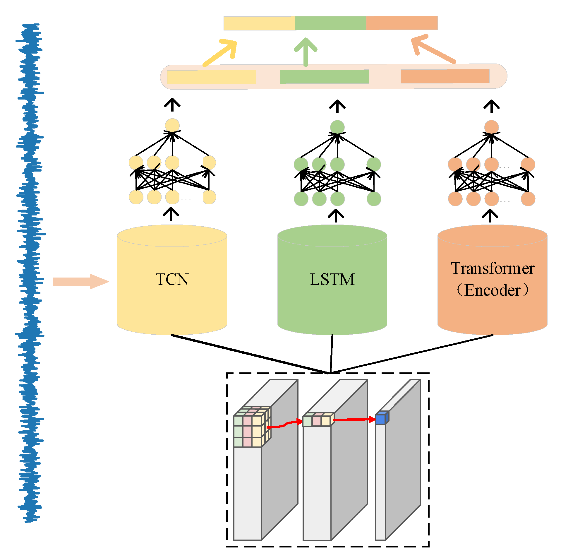
In order to get the prediction model closer to how the bearing really operates, this paper constructs a parallel multi-branch feature learning network using TCN, LSTM, and Transformer. The feature extraction model needs to be able to handle multi-dimensional problems and have the ability to extract spatial and temporal data. In this paper, a combination of TCN, LSTM, and Transformer is used for parallel processing of the models, and then fusion of their features can extract a rich feature representation that fully captures the advantages of different models. Where TCN performs feature extraction at different time steps through convolutional layers, which can capture both local and global temporal dependencies, LSTM is suitable for capturing long-range temporal features by creating long-term dependencies in the sequence through cyclic cells; Transformer, on the other hand, interacts globally with features in a sequence through a self-attentive mechanism that is able to capture global contextual relationships. With the parallel TCN-LSTM-Transformer network, multiple levels of features can be extracted at the same time, resulting in a richer and more comprehensive representation capability. The model schematic of this parallel feature extractor is shown in Figure 7.

3.3. Parallel Multi-Scale Attention Mechanisms

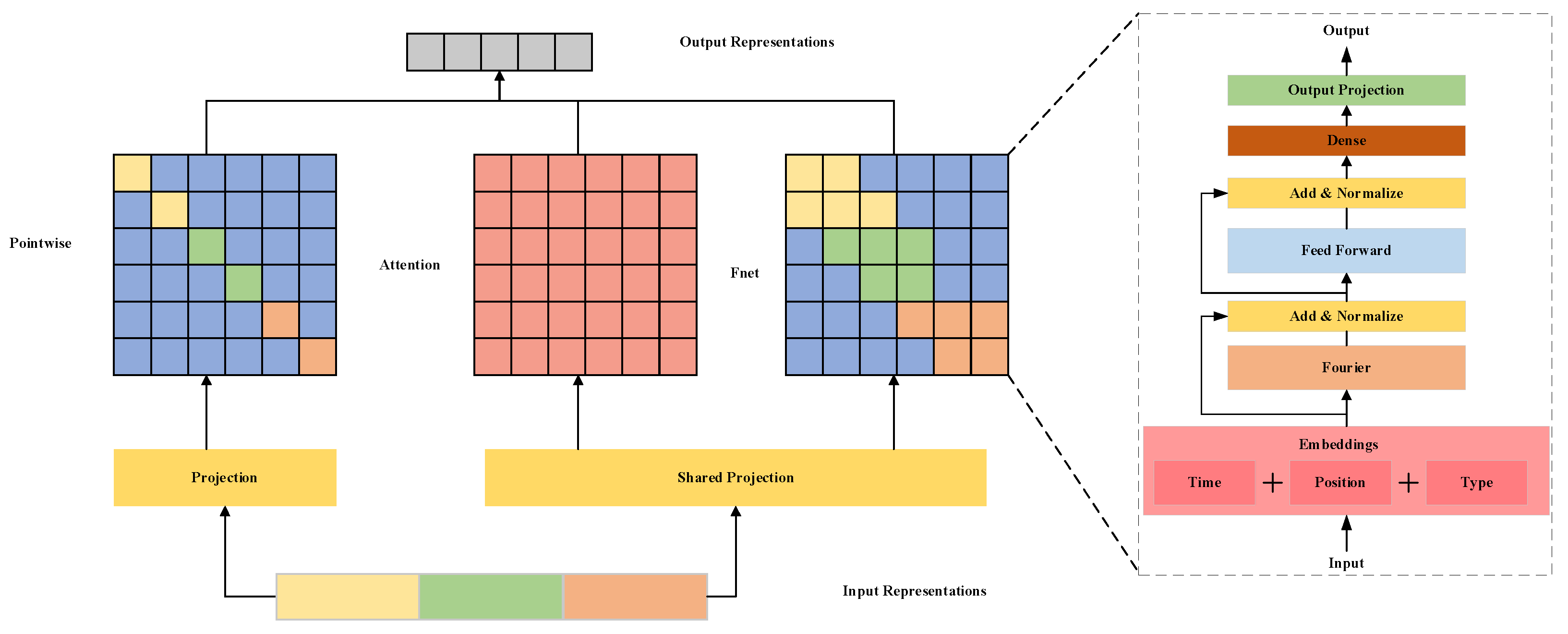
In most of the parallel attention mechanism structure research, each branch network is the same through the multi-head self-attention mechanism, which is used to adjust the internal relationships within the data. If you use the same feature extraction method for the fusion of the output of each branch network, it will lead to the important features not being highlighted and the redundant features being retained. Inevitably, the performance of the whole network would be impacted. To tackle this issue, this research proposes the development of a novel parallel, multi-scale attention method. The principle of its attention mechanism is shown in Figure 8.
FNet [25] replaces the self-attention layer with a Fourier sublayer, which speeds up the Transformer’s encoder with less loss of accuracy; however, FNet may lose some positional information when processing the sequence data, which will affect the precision of the RUL forecast. As a result, a parallel multi-scale attention mechanism is proposed in this paper, inspired by FNet. In order to increase the speed while reducing the loss of accuracy, the attention mechanism is implemented in conjunction with the FFT of the input features because the Fourier transform is faster than the calculation of the convolution and attention mechanism, which not only accelerates the training speed of the model but also enhances the feature extraction capability and stability. Utilizing self-attention and FNet, the process of encoding sequences concurrently at several sizes. Self-attention and FNet can be combined to learn sequence representations at a greater variety of scales. It consists of three primary components: self-attention, which captures global characteristics in the temporal domain; an FNet module for capturing local deep features in the frequency domain; and a feed-forward network used to capture positional characteristics. The module receives as input the result obtained from the -layer and produces an output representation in the form of a fused manner:
X i = X i 1 + A t t e n t i o n ( X i 1 ) + F N et ( X i 1 ) + P o int w i s e ( X i 1 )
where “Attention” pertains to the mechanism of self-attention, “FNet” denotes the FNet module, and “Pointwise” denotes the position feed-forward network. Below are the specifics of FNet and the FNet structure shown in Figure 8.
Given a sequence { x n } , n [ 0 , N 1 ] , the discrete Fourier transform (DFT) can be defined as follows:
X ( a ) = n = 0 N 1 x n e 2 π i N n a , 0 a N 1
where X ( a ) denotes the data after DFT. From Equation (18), the time complexity of DFT is O ( N 2 ) . FFT is a fast algorithm for discrete Fourier transform, which recursively obtains the result by butterfly operation, which reduces the number of DFT multiplications and the time complexity to O ( N log N ) .

3.4. RUL Forecast

Figure 5 illustrates the procedure for model training and predicting the RUL. The fusion of bearing vibration data obtained from multiple sensors yields multi-sensor fusion data. Consequently, this leads to the fulfillment of the prediction objective. In the RUL prediction process in Figure 5, the gathered bearing vibration data from many sensors is combined via fusion, resulting in multi-sensor fusion data. This data is then separated into training-bearing data and test-bearing data to construct the prediction network.
In the offline modeling process, the training data are input into the parallel feature extractor and trained several times. The training process calculates the loss function and backpropagation to adjust the model parameters, and once the number of training iterations exceeds the total number of training iterations, the model finishes the training process. In the online prediction process, the trained prediction network model is used to make real-time predictions by inputting test data. Furthermore, assessment indicators are established to validate the model’s predictive performance. Ultimately, the forecast outcomes are presented in a graphical representation.
In this study, bearings’ complete life cycle information is used to educate the network. The advantages are: (1) Complete life cycle data encompasses every conceivable bearing failure. Therefore, the examination of complete life cycle data will facilitate a more exhaustive surveillance of the bearing’s condition. (2) It has been noted that the duration between the initial injury and the ultimate failure of a bearing is exceptionally brief. Damage can spread rapidly, particularly when the bearing is on the verge of total failure. Hence, predicting the RUL before the onset of deterioration may provide enough time to schedule equipment repair. (3) Li et al. [26] used the concept of first prediction time (FPT) to classify life cycle data into two distinct stages: healthy and deteriorated. However, accurately establishing the FPT is a challenging endeavor that may require a significant increase in effort to calculate it manually. This research circumvents this issue by training the network utilizing comprehensive data over the whole lifespan.
The assessment metrics consist of mean absolute error (MAE) and root mean square error (RMSE). These metrics are described as follows:
M A E = 1 n i = 1 n | R u l i p r e R u l i a c t |
R M S E = 1 n i = 1 n ( R u l i p r e R u l i a c t ) 2
where R u l i a c t represents the actual value of the remaining life, R u l i p r e represents the predicted value of the remaining life, and n represents the overall duration of the prediction, which is equivalent to the number of samples. In addition, early RUL predictions and late RUL predictions have different impacts on the machine during the machinery and equipment’s actual operation. Therefore, in the early stages of the machine’s life cycle, the weight of the predicted results is reduced, while in the later stages, the weight of the predicted results is increased to capture possible malfunctions and failures of the machine more accurately. The scoring function’s definition is extracted from reference [21]. The scoring function designed in reference [21] differs from the scoring function in PHM 2012 [27] in that it takes into account the effects of the early stages of the machine lifecycle, the later stages of the machine lifecycle, and the whole lifecycle operation stages. The specific descriptions are shown in Equations (21) and (22):
A i = { exp ( ln ( 0.6 ) ( R u l i p r e Rul i a c t i 10 ) ) , e r i 0 exp ( ln ( 0.6 ) ( R u l i p r e R u l i a c t 40 ) ) , e r i > 0
S core = α 1 m i = 1 m A i + β 1 n m m + 1 n A i
where the weights of the early and late bearing phases are denoted by α and β , respectively, while the early stage proportion is represented by m . Here, α is set to 0.35 and β to 0.65, i.e., the late stage of the life cycle is predicted to be more significant than its early stage, and the higher the score, the more accurate the forecast.

4. Experimental Verification

In this section, we use the PHM 2012 Challenge dataset provided via the Association of Electrical and Electronics Engineers as well as the Bearing Degradation dataset provided by Xi’an Jiaotong University to verify the suggested method’s capacity for prediction. In addition, the framework of the Deep Learning Torch is used to perform the experiments. The computer is equipped with an i5-13400F CPU, an NVIDIA GeForce RTX 3060 Ti processor, and 16 GB of RAM.

4.1. Parameter Configuration of Multi-Feature Fusion Networks

In both cases, the hyperparameters of the multi-feature fusion network are the same, as detailed in Table 1. The hyperparameters were selected using cross-validation of numerous training datasets, taking into account the prediction accuracy.

4.2. Case Study 1: Predicting the RUL of Bearings Using the PHM 2012 Dataset

4.2.1. Introduction to the Dataset

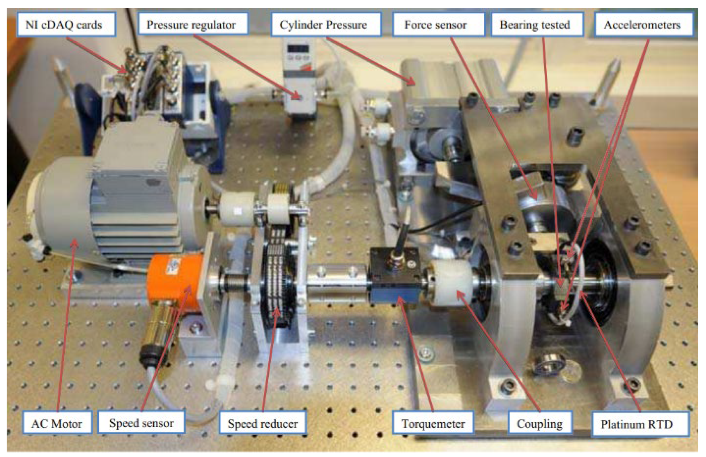
The bearing dataset for the IEEE PHM 2012 Data Challenge was acquired from the PRONOSTIA test platform, and the data acquisition platform is shown in Figure 9. The vibration acceleration data of rolling bearings during their whole life cycle, from normal operation to failure, under various operating situations, are obtained by the accelerated life degradation test, and the test is halted when the magnitude of the vibration signal surpasses 20 g. The vibration signals obtained are segregated into horizontal and vertical orientations. The data is sampled at a frequency of 25.6 kHz, with recordings taken every 10 s; the time duration of the collection is 0.1 s; and there are 2560 pieces of vibration data collected each time. Table 2 displays the data set’s operational circumstances.

4.2.2. Analysis of Projected Results

To comprehensively evaluate the performance of our prediction network, we carefully selected bearing vibration data from two different operating conditions, namely Condition 1 and Condition 2. Under these two conditions, we conducted five test experiments on each bearing to ensure the reliability of the data and the stability of the experimental results. Notably, in each experiment, we used a brand-new, untrained network. This approach was taken to ensure the consistency and repeatability of our experimental results.
When testing a specific bearing data set, we used the data from all other bearings to train the network. For example, if bearing A1-1 was chosen as the test set, then bearings A1-2, A1-3, A1-4, A1-5, A1-6, and A1-7 were used as the training set. This strategy ensured that each bearing data set could be used both for training and testing, maximizing the utilization of data and enhancing the effectiveness of the experiments.
To demonstrate the effectiveness of our method, we selected four different approaches and compared their RUL prediction results with our multi-feature fusion-based prediction results. The specific comparison results are shown in Table 3.
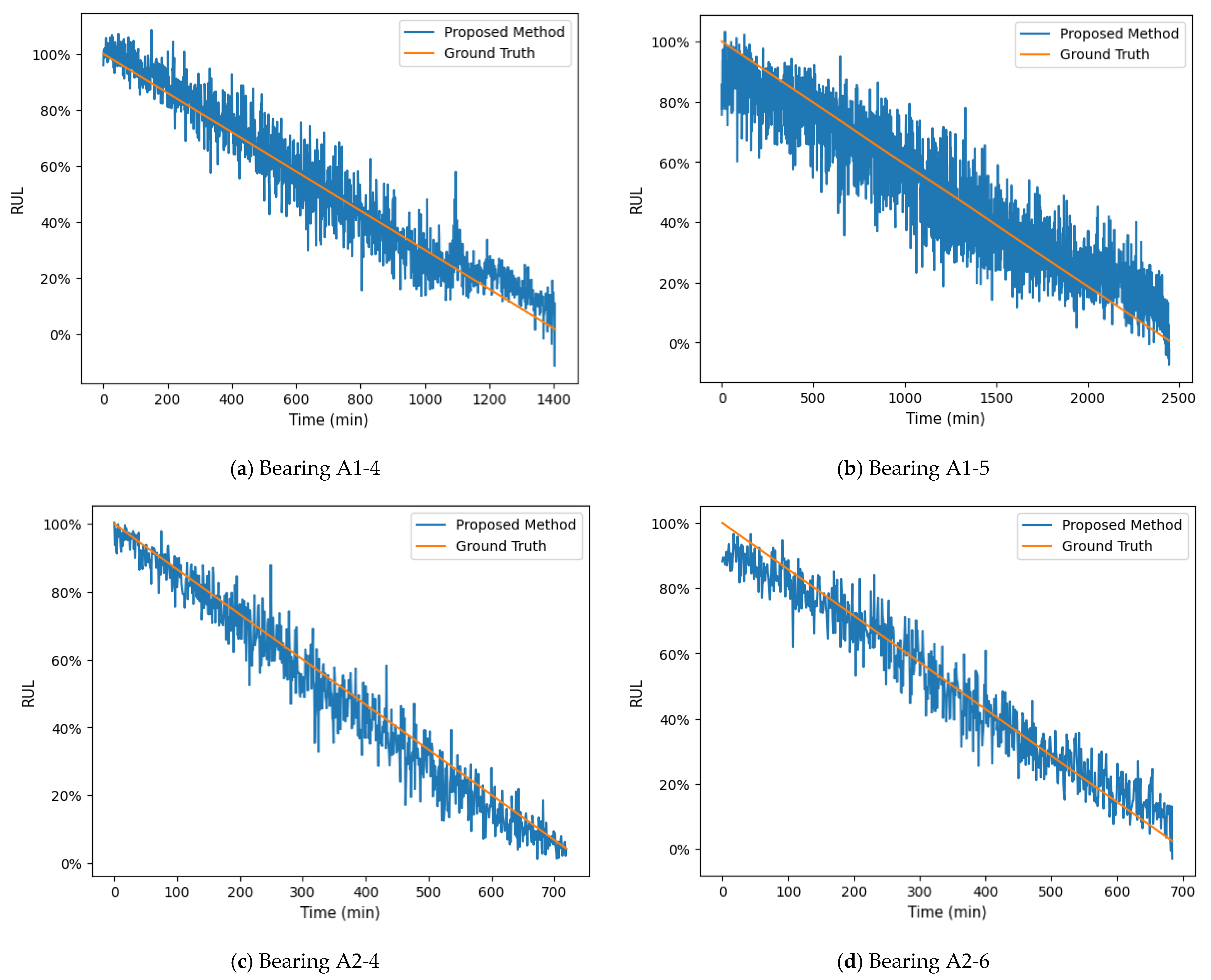
In this experiment, a total of 14 bearings were examined. As Table 3 illustrates, for most of the tested bearings, the proposed approach’s MAE and RMSE are less than those of the comparison method, and as Figure 10 illustrates, the proposed method’s average RMSE and MAE are the lowest while its score is the greatest. The approach suggested in this paper has greater score values than the comparable methods, except that the score of tests bearing A1-1 is lower than that of TCN-RSCB and the score of tests bearing A2-3 is the same as that of TCN-RSCB. The aforementioned experimental findings demonstrate that the proposed method has the greatest prediction performance because the multi-sensor data fusion method effectively fuses multi-sensor data, and in the multi-feature fusion network, we designed a parallel TCN-LSTM-Transformer feature extractor. Where TCN extracts the data’s long-term sequence features, LSTM captures the time-dependent features in the sequence data, and Transformer extracts the global feature representation of the bearing data. Meanwhile, a parallel multi-scale attention mechanism is designed that captures both local and global dependencies to go a step further in capturing the global and local contextual information of the sequence in order to accomplish the three feature extractors’ output features’ adaptive weighted fusion. Secondly, the shallow features obtained from the parallel feature extractor are residually connected to the deep features through the attention mechanism to improve the efficiency of utilizing the information of the front and back features, and finally, the RUL’s output is used in the fully connected layer. Among them, CNNs face the drawbacks of insufficient modeling power for long-term dependence, fixed sense field size, a large number of parameters, and translational invariance, leading to poor RUL prediction when dealing with time series data. Although TCN-SA, TCN-RSA, and TCN-RSCB introduce attention mechanisms and residual connections to improve the traditional TCN models, they have some drawbacks, such as not considering the global nature, not mining the information more deeply, and not utilizing the before and after feature information efficiently. In conclusion, the multi-feature fusion network gets higher forecast results due to the design of the multi-feature fusion network, which enhances the all-round learning of sequence features, the attention mechanism’s deep feature mining, and the improvement of the efficiency of residual linkage in the utilization of before and after features. Furthermore, even if the proposed method’s prediction curves exhibit some local oscillations, the proposed approach has a good capacity to anticipate the RUL of the bearings since it can accurately estimate the condition of the bearings in their latter stages of life.
The prediction results for bearings A1-4, A1-5, A2-4, and A2-6 are shown in Figure 11. Figure 11 demonstrates that our proposed multi-feature fusion network successfully captures the bearing degradation information across various operating situations and accurately predicts the RUL.

4.2.3. Ablation Experiment

To evaluate the efficacy of the novel aspect of the proposed methodology, we eliminated or altered a component of the methodology. Data for the ablation experiments were obtained from the PHM 2012 dataset with test bearings A1-4. Method 1 utilizes vertical vibration data obtained from a solitary vertical sensor as input, whereas the proposed method uses multi-sensor fusion data as input. Method 2 utilizes TCN blocks for network feature extraction; the proposed method uses TCN-LSTM-Transformer for network feature extraction. Method 3 uses the traditional self-attention mechanism for feature fusion; the proposed method uses a parallel multi-scale attention mechanism in order to accomplish the adaptive weighted fusion of the output features from the three feature extractors. The prediction findings are shown in Table 4, revealing that the MAE and RMSE outcomes of the proposed approach are markedly superior to those of the comparable approaches.

4.3. Case Study 2: Predicting the RUL of Bearings Using the XJTU-SY Dataset

4.3.1. Introduction to the Dataset

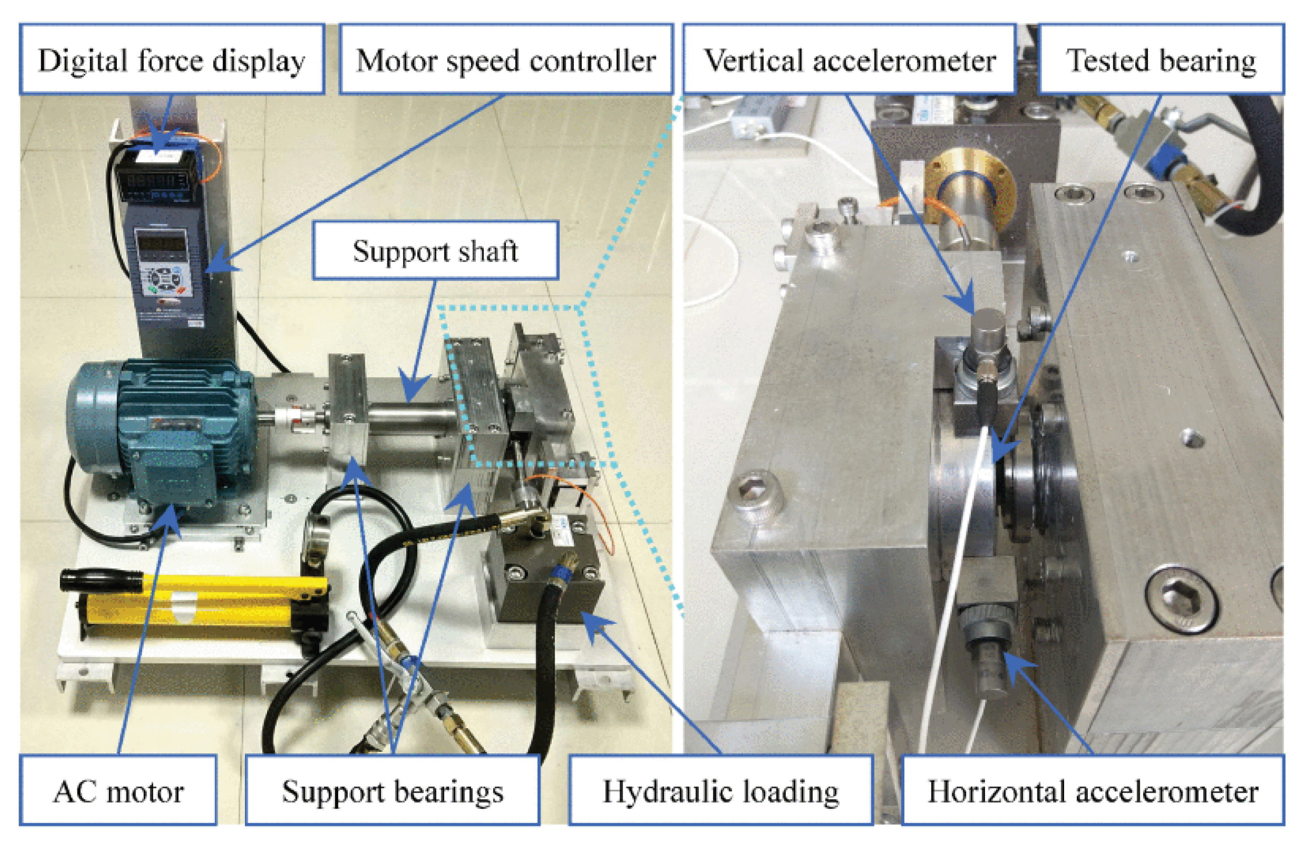
Data set for the XJTU-SY rolling bearing accelerated life test [30]. The test rig for this collected dataset is shown in Figure 12. The platform is used to perform accelerated degradation tests on bearings by generating radial force from a hydraulic loading system, and the AC motor’s speed is controlled by its speed controller. The gathered vibration signals were split into horizontal and vertical directions, and the test’s sample frequency was set to 25.6 kHz, the sampling interval was set at 1 min, and the sampling time was 1.28 s. Figure 13 shows the physical diagrams of bearing inner ring wear, cage fracture, outer ring wear, and outer ring cracking. Different deterioration patterns under various operating situations are caused by these bearing degradation trends. Two different operating conditions were selected for the XJTU-SY test, as shown in Table 5. For the first scenario, the motor speed is 2100 r/min, and the load is 12 kN; for the second scenario, the motor speed is 2250 r/min, and the load is 11 kN; both conditions contain five different bearings each.

4.3.2. Analysis of Projected Results

To assess the prediction network’s generalization capacity to the fullest extent possible, the bearing vibration data under Cases 1 and 2 were selected from the working conditions. When RUL prediction is performed using the XJTU-SY dataset, the network parameters, MAE, RMSE, and scoring function of multi-feature fusion are identical to those of Case 1. In addition, the proposed method’s superiority is shown by comparing the multi-feature fusion prediction results with those of the four approaches in Case 1, and Table 6 displays the outcomes of their predictions.
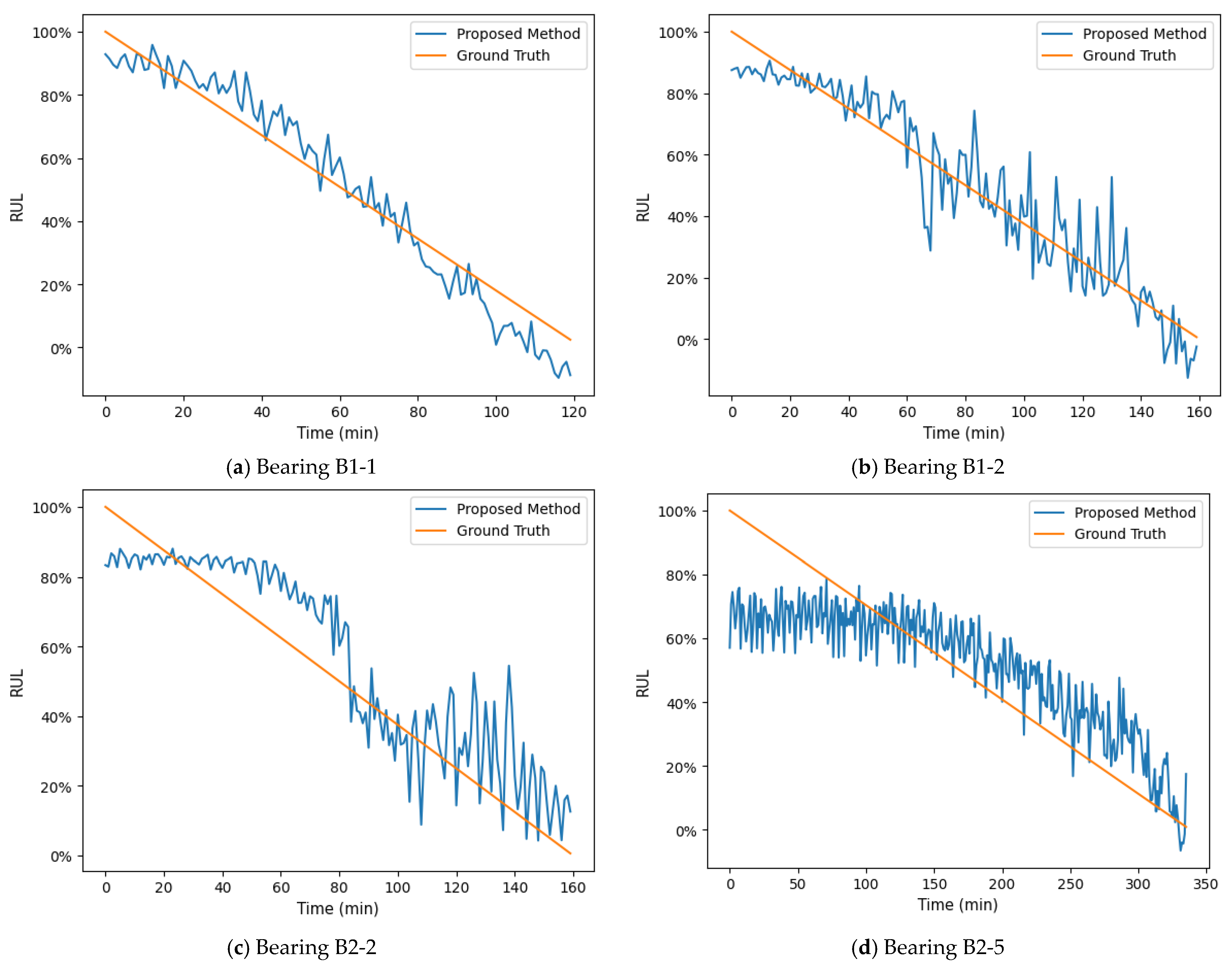
In this experiment, a total of 10 bearings were subjected to testing. Table 6 demonstrates that the proposed method exhibits reduced MAE and RMSE values compared to the comparison method for the majority of the tested bearings. Figure 14 clearly demonstrates that the proposed method achieves the lowest average MAE and average RMSE while also attaining the greatest score. This suggests that the proposed approach exhibits superior performance in predicting the RUL of bearings. The scoring values of the proposed method in this paper surpass those of the comparison methods, except that the score of tests bearing B1-1 is lower than that of TCN-SA, B2-5 is lower than that of TCN-RSCB, and the score of tests bearing B1-5 is the same as that of TCN-SA. Furthermore, due to the diverse range of failures that bearings often experience as they degrade, it is very challenging for prediction methods to accurately determine the optimal RUL forecast for any individual bearing. Figure 15 displays the RUL forecast outcomes for the B1-1, B1-2, B2-2, and B2-5 bearings. Despite the presence of local oscillations in the curves of the proposed method, accurate predictions may be made on the state of the bearings throughout the latter stages of their service life. Ultimately, the proposed method demonstrates a commendable capacity to anticipate the RUL of rolling bearings.

4.3.3. Ablation Experiment

To assess the suggested method’s ability for generalization, the design of the ablation trials aligns with the PHM 2012 dataset, and the test bearing selected is B1-2. Table 7 displays the outcomes of the predictions, revealing that the MAE and RMSE outcomes of the proposed method exhibit a notable superiority over those of the comparative methods.

5. Conclusions

In order to improve the real-time monitoring capability in industrial processes and accurately and efficiently identify the rolling bearings’ state of health during operation, a multi-feature fusion-based rolling bearing RUL prediction method is put forward. The following conclusions are drawn from the experimental findings based on the PHM 2012 bearing degradation dataset and the XJTU-SY bearing accelerated life test dataset:
(1)
A method for multi-sensor data fusion has been developed to combine data from many sensors based on their channels. This approach not only provides an effective fusion of multi-sensor data but also compensates for the limitations of standard prediction methods that rely only on data from a single sensor.
(2)
To address the issue of incomplete extraction of global feature information throughout the feature extraction procedure, this paper uses TCN, LSTM, and Transformer to construct a parallel multi-branch feature learning network, designs a parallel multi-scale attention mechanism to capture both local and global dependencies, and realizes the adaptive weighted fusion of the output features from three types of feature extractors. The shallow features obtained by the parallel feature extractor are then residually connected with the deeper features through the attention mechanism to improve the utilization efficiency of the before and after feature information so as to learn more comprehensive feature information.
(3)
Validation of the validity and generalization ability of the proposed method using the PHM 2012 bearing degradation dataset and the XJTU-SY bearing accelerated life test dataset. The experimental findings demonstrate that the proposed method can precisely forecast the RUL of a variety of bearings. Comparative experiments demonstrate that the proposed method has a reduced prediction error.

Author Contributions

Conceptualization, D.J. and G.Z.; methodology, G.Z.; software, G.Z.; validation, G.Z.; formal analysis, G.Z.; investigation, G.Z.; resources, G.Z.; data curation, G.Z.; writing—original draft preparation, G.Z.; writing—review and editing, G.Z.; visualization, G.Z.; supervision, D.J.; project administration, D.J.; funding acquisition, D.J. All authors have read and agreed to the published version of the manuscript.

Funding

This research was funded by the National Science Foundation of China (62263020), the Key R&D Program of Gansu Province (23YFGA0061), the Lanzhou Science and Technology Plan Project (2022-2-69), and the Excellent Youth Foundation of Gansu Scientific Committee (20JR10RA202).

Data Availability Statement

The data used for training and test set PHM 2012 are available at: https://github.com/Lucky-Loek/ieee-phm-2012-data-challenge-dataset (accessed on 20 January 2024). The data used for training and test set SJTU-SY are available at: https://github.com/WangBiaoXJTU/xjtu-sy-bearing-datasets (accessed on 20 January 2024).

Conflicts of Interest

The authors declare no conflicts of interest.

Correction Statement

This article has been republished with a minor correction to the readability of Figures 5 and 6. This change does not affect the scientific content of the article.

References

  1. Lei, Y.G.; Jia, F.; Kong, D.T.; Ling, J.; Xing, S.B. Opportunities and challenges of mechanical intelligent fault diagnosis under big data. J. Mech. Eng. 2018, 54, 94–104. (In Chinese) [Google Scholar] [CrossRef]
  2. Fragoso, A.; Martins, R.F.; Soares, A.C. Failure analysis of a ball mill located in a cement’s production line. Eng. Fail. Anal. 2022, 138, 106339. [Google Scholar] [CrossRef]
  3. Saucedo-Dorantes, J.J.; Arellano-Espitia, F.; Delgado-Prieto, M.; Osornio-Rios, R.A. Diagnosis methodology based on deep feature learning for fault identification in metallic, hybrid and ceramic bearings. Sensors 2021, 21, 5832. [Google Scholar] [CrossRef]
  4. Shi, H.T.; Hou, M.X.; Wu, Y.H.; Li, B.C. Incipient fault detection of full ceramic ball bearing based on modified observer. Int. J. Control Autom. Syst. 2022, 20, 727–740. [Google Scholar] [CrossRef]
  5. Zhang, X.C.; Wu, D.; Xia, Z.F.; Li, Y.F.; Wang, J.Q.; Han, E.H. Characteristics and mechanism of surface damage of hybrid ceramic ball bearings for high-precision machine tool. Eng. Fail. Anal. 2022, 142, 106784. [Google Scholar] [CrossRef]
  6. Si, X.S.; Wang, W.B.; Hu, C.H.; Zhou, D.H. Remaining useful life estimation–A review on the statistical data driven approaches. Eur. J. Oper. Res. 2011, 213, 1–14. [Google Scholar] [CrossRef]
  7. Singleton, R.K.; Strangas, E.G.; Aviyente, S. Extended Kalman filtering for remaining-useful-life estimation of bearings. IEEE Trans. Ind. Electron. 2014, 62, 1781–1790. [Google Scholar] [CrossRef]
  8. Chen, C.C.; Vachtsevanos, G.; Orchard, M.E. Machine remaining useful life prediction: An integrated adaptive neuro-fuzzy and high-order particle filtering approach. Mech. Syst. Signal Process. 2012, 28, 597–607. [Google Scholar] [CrossRef]
  9. Cai, B.P.; Fan, H.Y.; Shao, X.Y.; Liu, Y.H.; Liu, G.J.; Liu, Z.K.; Ji, R.J. Remaining useful life re-prediction methodology based on Wiener process: Subsea Christmas tree system as a case study. Comput. Ind. Eng. 2021, 151, 106983. [Google Scholar] [CrossRef]
  10. Le Son, K.; Fouladirad, M.; Barros, A. Remaining useful lifetime estimation and noisy gamma deterioration process. Reliab. Eng. Syst. Saf. 2016, 149, 76–87. [Google Scholar] [CrossRef]
  11. Kundu, P.; Darpe, A.K.; Kulkarni, M.S. Weibull accelerated failure time regression model for remaining useful life prediction of bearing working under multiple operating conditions. Mech. Syst. Signal Proc. 2019, 134, 106302. [Google Scholar] [CrossRef]
  12. Sun, Q.Q.; Ge, Z.Q. A survey on deep learning for data-driven soft sensors. IEEE Trans. Industr. Inform. 2021, 17, 5853–5866. [Google Scholar] [CrossRef]
  13. Deutsch, J.; He, D. Using deep learning-based approach to predict remaining useful life of rotating components. IEEE Trans. Syst. Man Cybern. 2017, 48, 11–20. [Google Scholar] [CrossRef]
  14. Hinton, G.E.; Osindero, S.; Teh, Y.W. A fast learning algorithm for deep belief nets. Neural Comput. 2006, 18, 1527–1554. [Google Scholar] [CrossRef]
  15. Guo, L.; Li, N.P.; Jia, F.; Lei, Y.G.; Lin, J. A recurrent neural network based health indicator for remaining useful life prediction of bearings. Neurocomputing 2017, 240, 98–109. [Google Scholar] [CrossRef]
  16. Catelani, M.; Ciani, L.; Fantacci, R.; Patrizi, C.; Picano, B. Remaining useful life estimation for prognostics of lithium-ion batteries based on recurrent neural network. IEEE Trans. Instrum. Meas. 2021, 70, 3524611. [Google Scholar] [CrossRef]
  17. Hochreiter, S.; Schmidhuber, J. Long short-term memory. Neural Comput. 1997, 9, 1735–1780. [Google Scholar] [CrossRef]
  18. Miao, H.H.; Li, B.; Sun, C.; Liu, J. Joint learning of degradation assessment and RUL prediction for aeroengines via dual-task deep LSTM networks. IEEE Trans. Industr. Inform. 2019, 15, 5023–5032. [Google Scholar] [CrossRef]
  19. Ren, L.; Dong, J.B.; Wang, X.K.; Meng, Z.H.; Zhao, L.; Deen, M.J. A data-driven auto-CNN-LSTM prediction model for lithium-ion battery remaining useful life. IEEE Trans. Industr. Inform. 2020, 17, 3478–3487. [Google Scholar] [CrossRef]
  20. Bai, S.J.; Kolter, J.Z.; Koltun, V. An empirical evaluation of generic convolutional and recurrent networks for sequence modeling. arXiv 2018, arXiv:1803.01271. [Google Scholar]
  21. Wang, Y.W.; Deng, L.; Zheng, L.Y.; Gao, R.X. Temporal convolutional network with soft thresholding and attention mechanism for machinery prognostics. J. Manuf. Syst. 2021, 60, 512–526. [Google Scholar] [CrossRef]
  22. Mo, Y.; Wu, Q.H.; Li, X.; Huang, B.Q. Remaining useful life estimation via transformer encoder enhanced by a gated convolutional unit. J. Intell. Manuf. 2021, 32, 1997–2006. [Google Scholar] [CrossRef]
  23. Egea-Lopez, E.; Martinez-Sala, A.; Vales-Alonso, J.; Garcia-Haro, J.; Malgosa-Sanahuja, J. Wireless communications deployment in industry: A review of issues, options and technologies. Comput. Ind. 2005, 56, 29–53. [Google Scholar] [CrossRef]
  24. Li, N.P.; Gebraeel, N.; Lei, Y.G.; Fang, X.L.; Cai, X.; Yan, T. Remaining useful life prediction based on a multi-sensor data fusion model. Reliab. Eng. Syst. Saf. 2021, 208, 107249. [Google Scholar] [CrossRef]
  25. Lee-Thorp, J.; Ainslie, J.; Eckstein, I.; Ontañón, S. Fnet: Mixing tokens with fourier transforms. arXiv 2021, arXiv:2105.03824. [Google Scholar]
  26. Li, X.; Zhang, W.; Ding, Q. Deep learning-based remaining useful life estimation of bearings using multi-scale feature extraction. Reliab. Eng. Syst. Saf. 2019, 182, 208–218. [Google Scholar] [CrossRef]
  27. Nectoux, P.; Gouriveau, R.; Medjaher, K.; Ramasso, E.; Chebel-Morello, B.; Zerhouni, N.; Varnier, C. An experimental platform for bearings accelerated degradation tests. In Proceedings of the IEEE International Conference on Prognostics and Health Management IEEE (ICPHM), Beijing, China, 23–25 May 2012; pp. 23–25. [Google Scholar]
  28. Cao, Y.D.; Ding, Y.F.; Jia, M.P. A novel temporal convolutional network with residual self-attention mechanism for remaining useful life prediction of rolling bearings. Reliab. Eng. Syst. Saf. 2021, 215, 107813. [Google Scholar] [CrossRef]
  29. Zhang, Y.Z.; Zhao, X.Q. Remaining useful life prediction of bearings based on temporal convolutional networks with residual separable blocks. J. Braz. Soc. Mech. Sci. 2022, 44, 527. [Google Scholar] [CrossRef]
  30. Lei, Y.G.; Han, T.Y.; Wang, B.; Li, N.P.; Yan, T.; Yang, J. Interpretation of XJTU-SY rolling bearing accelerated life test dataset. J. Mech. Eng. 2019, 55, 1–6. [Google Scholar]
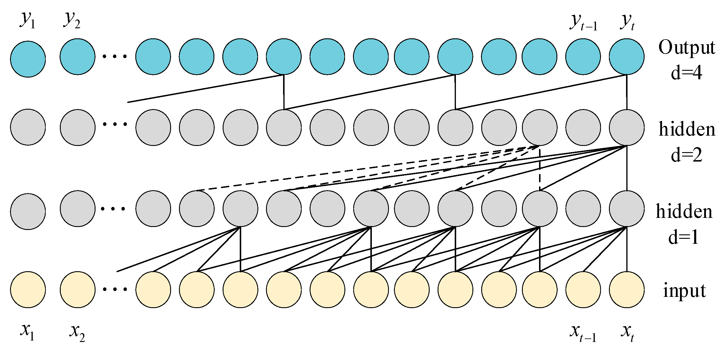
Figure 1. Illustration of the dilated causal convolution operation.
Applsci 14 01294 g001
Figure 2. Schematic diagram of the residual block in TCN.
Applsci 14 01294 g002
Figure 3. LSTM neural network.
Applsci 14 01294 g003
Figure 4. Structure of the Transformer encoder.
Applsci 14 01294 g004
Figure 5. The proposed method’s RUL prediction mechanism.
Applsci 14 01294 g005
Figure 6. Fusion of data from multiple sensors via channel fusion.
Applsci 14 01294 g006
Figure 7. The diagram of the hybrid neural network.
Applsci 14 01294 g007
Figure 8. The schematic diagram of the parallel multi-scale attention mechanism.
Applsci 14 01294 g008
Figure 9. PHM 2012 dataset-bearing test bench.
Applsci 14 01294 g009
Figure 10. Boxplots of MAE, RMSE, and scores on the PHM2012 dataset.
Applsci 14 01294 g010
Figure 11. The PHM 2012 dataset contains RUL visualization prediction results for test bearings.
Applsci 14 01294 g011
Figure 12. Bearing test bench of the XJTU-SY dataset.
Applsci 14 01294 g012
Figure 13. Failure photos of bearings.
Applsci 14 01294 g013
Figure 14. Boxplots of MAE, RMSE, and scores on the XJTU-SY dataset.
Applsci 14 01294 g014
Figure 15. The XJTU-SY dataset contains RUL visualization prediction results for test bearings.
Applsci 14 01294 g015
Table 1. Parameters of a multi-feature fusion network model.
ModuleLayerParameters
TransformerBatchNorm1dNum_eatures: 2560
Eps: 1 × 10⁻⁵
Momentum: 0.1
affine: True
Track running stats: True
Transformer Encoder
Layer
D_model: 2
Nhead: 2
Dim feedforward: 2048
Dropout: 0.1
Activation: relu
Normalize before: False
Num layers: 3
LinearIn features: 5120
Out features: 1
Bias: True
TCNTemporal BlockN_inputs: 2560
N_outputs: 8
kernel_size: 3
Stride: 1
dilation: 1, 2, 4
dropout: 0.5
Temporal Conv NetNum_inputs: 2560
Num_channels: 8, 8, 8
Kernel_size: 3
Dropout: 0.2
LSTMNor: 2560
input features: 2
number of hidden states: 3
number of input features: 7680
Hidden Size: 3
Flatten
FNetDim: 100
Depth: 3
Mlp_dim: 100
Dropout: 0
Table 2. The FEMTO-ST bearing dataset’s operating conditions.
Operating ConditionA1A2A3
1800 r/min
4000 N
1650 r/min
4200 N
1500 r/min
5000 N
BearingBearing A1-1Bearing A2-1Bearing A3-1
Bearing A1-2Bearing A2-2Bearing A3-2
Bearing A1-3Bearing A2-3Bearing A3-3
Bearing A1-4Bearing A2-4
Bearing A1-5Bearing A2-5
Bearing A1-6Bearing A2-6
Bearing A1-7Bearing A2-7
Table 3. Results of several algorithms’ predictions in the PHM 2012 dataset.
Test SetTCN-SA [21]TCN-RSA [28]Standard-CNNTCN-RSCB [29]Proposed Method
MAERMSEScoreMAERMSEScoreMAERMSEScoreMAERMSEScoreMAERMSEScore
A1-110.411.30.8711.013.70.848.710.90.848.610.70.888.7211.50.87
A1-213.016.90.8014.016.30.7912.116.10.589.612.80.7110.914.70.85
A1-39.711.70.8111.414.10.7815.318.20.8311.714.10.856.708.340.88
A1-47.18.50.7313.715.80.595.737.370.836.908.400.825.747.310.85
A1-59.1113.00.8310.913.20.809.5113.00.7411.514.20.768.4512.80.84
A1-68.311.90.688.411.10.7012.215.30.608.2310.60.7714.518.00.82
A1-79.012.90.7517.823.50.7817.621.90.7313.919.20.8113.218.00.83
A2-114.318.10.7429.035.30.7333.639.90.6922.327.90.7419.526.10.78
A2-214.518.60.4417.221.40.4717.521.60.4510.213.90.6911.916.70.70
A2-317.923.00.7724.430.80.7519.827.00.7216.522.90.7916.119.40.79
A2-45.186.420.916.58.10.826.057.580.806.278.280.884.946.300.92
A2-513.316.10.7815.218.90.6717.421.70.7512.516.10.783.834.810.89
A2-610.913.80.8312.214.30.7614.518.60.768.1010.70.843.755.070.90
A2-717.525.00.5318.624.10.468.6110.40.728.2010.00.777.389.230.83
Average11.414.80.7515.018.60.7114.217.80.7211.014.20.7910.413.50.83
Table 4. Results of ablation experiments with different comparison methods under the PHM2012 dataset.
Method 1Method 2Method 3Proposed Method
MAE13.48.716.325.74
RMSE14.59.438.517.31
Table 5. Operating conditions for the SJTU-SY bearing dataset.
Operating ConditionB1B2B3
2100 r/min
12 kN
2250 r/min
11 kN
2400 r/min
10 kN
bearingBearing B1-1Bearing B2-1Bearing B3-1
Bearing B1-2Bearing B2-2Bearing B3-2
Bearing B1-3Bearing B2-3Bearing B3-3
Bearing B1-4Bearing B2-4Bearing B3-4
Bearing B1-5Bearing B2-5Bearing B3-5
Table 6. Prediction results of different methods in the XJTU-SY dataset.
Test SetTCN-SA [21]TCN-RSA [28]Standard-CNNTCN-RSCB [29]Proposed Method
MAERMSEScoreMAERMSEScoreMAERMSEScoreMAERMSEScoreMAERMSEScore
A1-15.27.10.9021.525.90.7514.316.60.7012.314.80.825.77.30.88
A1-219.024.00.8018.823.00.618.211.80.817.79.30.837.29.30.84
A1-317.021.70.6513.616.00.6516.118.90.618.410.00.698.29.70.71
A1-426.830.40.8011.914.00.6618.522.20.467.910.10.847.18.80.85
A1-520.325.30.5119.722.30.4528.233.60.3127.832.70.4019.221.40.51
A2-113.616.40.8023.729.50.6523.028.30.6420.824.90.7612.415.10.81
A2-214.518.60.8511.313.80.6814.316.70.758.210.20.868.610.60.86
A2-313.617.10.8521.824.40.7611.013.40.6610.815.40.8610.712.80.87
A2-416.619.40.7416.019.00.6416.520.80.6013.517.50.7914.416.60.80
A2-511.114.30.8018.322.80.7114.718.10.627.29.20.8111.514.90.78
Average15.819.40.7717.721.10.6616.520.00.6212.515.40.7710.512.60.79
Table 7. Results of ablation experiments with different comparison methods under the SJTU-SY dataset.
Method 1Method 2Method 3Proposed Method
MAE16.311.59.27.1
RMSE20.514.911.18.8
Disclaimer/Publisher’s Note: The statements, opinions and data contained in all publications are solely those of the individual author(s) and contributor(s) and not of MDPI and/or the editor(s). MDPI and/or the editor(s) disclaim responsibility for any injury to people or property resulting from any ideas, methods, instructions or products referred to in the content.