A Machine Learning Approach to Simulation of Mallard Movements

Abstract

Machine learning (ML) is increasingly used in diverse fields, including animal behavior research. However, its application to ambiguous data requires careful consideration to avoid uncritical interpretations. This paper extends prior research on ringed mallards where sensors revealed their movements in southern Sweden, particularly in areas with small lakes. The primary focus is to distinguish the movement patterns of wild and farmed mallards. While well-known statistical methods can capture such differences, ML also provides opportunities to simulate behaviors outside of the core study span. Building on this, this study applies ML techniques to simulate these movements, using the previously collected data. It is crucial to note that unrefined application of ML can lead to incomplete or misleading outcomes. Challenges in the data include disparities in swimming and flying records, farmed mallards’ biased data due to feeding points, and extended intervals between data points. This research highlights these data challenges, while identifying discernible patterns, as well as proposing approaches to meet such challenges. The key contribution lies in separating incompatible data and, through different ML models, handle these separately to enhance the reliability of the simulation models. This approach ensures a more credible and nuanced understanding of mallard movements, demonstrating the importance of critical analysis in ML applications in wildlife studies.

1. Introduction

A computer simulation uses a model mimicking a real system, representing the dynamics of that system, i.e., the simulation in execution forms a representation of the real behavior of the system [1]. Typically, simulation models are used to predict and study behaviors in response to conditions that otherwise cannot be easily or safely applied in a real-life setting. The main aim of this study is to find applicable and trustworthy machine learning (ML)-based simulation models for specific behaviors, here mallard movements.

Today, wildlife ecology studies generate an ever-increasing amount of data [2]. Due to this fact, analyzing is getting more challenging, not only because of the growing size of data, but also because data evolve into more complex data structures. Depending on the data, various models and techniques can be applied for dispersal and predicting animal migrations, usually ranging from statistics [3,4,5,6] to machine learning [2,7,8,9] and deep learning [10,11,12,13,14] models to spatial analysis techniques applied on GIS data [3,7,14,15] appearing in recent animal movement research, as well as already mentioned simulations [16,17].

McDuie et al. [3] used statistical methods like Pearson, chi-square, and ANOVA to estimate the distance moved, the area used, and how time was allocated throughout the day. Here, the variable of interest was the step length and the individual bird day for the sampling unit(s). Another statistical method, incorporating net squared displacement (NSD) statistics within a nonlinear hierarchical modeling framework, was used for modeling animal dispersal [4,5,6]. While this approach facilitated the efficient creation of precise population redistribution kernels, enabled the quantification of individual variations in dispersal, and permitted the testing of hypothesized correlations related to these variations, it is important to note that this model was not suitable for making predictions.

When we came to the use of machine learning in investigating animal migration, Valletta et al. [2] approached three cases using data covering pheasant eggs, jackdaw associations, and wildebeest identifications and applied both unsupervised and supervised machine learning. With large datasets and complex variables, Asmara et al. [7] found artificial neural networks (ANN), such as self-organizing maps (SOMs), useful for unstructured data and species distribution modeling of bird species at a Kenyir area. In an additional supervised learning study, Butts et al. [8] emphasized using and finding appropriate mathematical models for one deer and extrapolated this to model groups of deer through a so-called “data-driven agent-based” modeling approach. Huettmann et al. [9] looked at seasonal plot surveys for short-billed gull presence at Fairbanks in Alaska using classification and regression trees (CARTs), CART Ensembles and Bagger, TreeNet, random forests, and multivariate adaptive regression splines (MARS). The simulation models presented in [2,8] contributed to our studies and were the sources of inspiration for gaining insights into ML model approaches.

Wijeyakulasuriya et al. [10] used random forests, neural networks, and recurrent neural networks (RNNs) to compare performance in predicting one step ahead for migratory gulls’ data as well as long-range simulations for black carpenter ant movements. The RNNs were used for sequential data or time-series data. Work on animal movements has used further neural network techniques predicting movement and/or movement patterns. In Peng et al. [11], an RNN was used to classify movement patterns from the southern elephant seal species, and their neural network model was composed of two parts. The first part was an RNN that could extract features from the input trajectory segments. The second part included two single-layer neural networks, each of which was fed by the output of the aforementioned RNN. Maekawa et al. [12] used a deep learning software assistant tool for the comparative analysis of animal movements, segmenting trajectories and visualizing them to reveal underlying meanings and facilitating new hypotheses of behaviors. Especially, the scaling from millimeters to hundreds of kilometers revealed movement features of animals of various sizes. Furthermore, Rew et al. [13] used the spatiotemporal movement of long-billed curlew birds using RNN models and a random forest method, considering both observation points and environmental factors and filling in gaps for missing positional GPS data.

A theoretical model can be used on flocks or herds of animals, as presented by Amornbunchornvej and Berger-Wolf in [14], where they generated a set of time series of 2-dimensional x- and y-coordinates corresponding to longitude and latitude GPS positions. Applying the model to a herd of baboons showed good results. Further articles combining geographic information system (GIS) and geographic positioning system (GPS) sensor data have used various statistical and ML methods in combination for animal movement analytics. The authors mentioned before [3] compiled the data in an Environmental Systems Research Institute (ESRI) GIS platform with 68 open access predictor layers. An additional trend by Huang et al. [15] showed the development of geospatial artificial intelligence (AI) techniques, adding geographical features as input features to existing ML models/frameworks for animal and human movements, and in [7] showed relationships between movements and resource usage, landscape interactions, and specific habitat needs tracked via GPS–GSM transmitters to examine fine-scale movement patterns.

Sebastian Echegaray and Luo [16] presented a simulation involving the evolution of basic animal behavior in a prey–predator food model, where surviving animals breed successive generations, possessing sensors for environmental awareness and free movement. Xue et al. [17] used simulation for storm petrel behavior using morphological measurements and aerodynamic models, with deep reinforcement learning to demonstrate the petrel’s high maneuverability and stability under various wind conditions, offering insights into its biomechanics and guiding the design of biomimetic robots. Here, the authors applied the deep deterministic policy gradient (DDPG) algorithm, implemented in a simulation reinforcement learning toolbox in Matlab, i.e., the Simscape Multibody simulation environment (Matlab R2021b, MathWorks, Inc., Portola Valley, CA, USA).

ML is generally considered as a potential and efficient tool for processing extensive datasets across various domains, including industrial robotics [18], the internet of things and edge computing [19], and rack detection in bridge concrete [20]. Beyond these applications, as pointed out before, ML holds promise for contributing to fields like animal behavior and large-scale ecology systems [2], gaining popularity in these contexts and inspiring the focus of this contribution, that is, movements of wild and farmed mallards.

Traditionally, machine learning models have relied on plaintext data for training and predictions, potentially containing sensitive information. It should be mentioned that it is crucial to consider the security and privacy preservation in ML models. Reviews and surveys on the current state of knowledge regarding privacy preservation in ML workflows can be found, for example, in [21,22,23,24]. In privacy-preserving machine learning, the primary objective is to ensure the continuous encryption or maintenance of raw data in ciphertext form during both training and prediction processes. The term “ciphertext” refers to the encrypted form of data. In this context, the advancements allow for the training and prediction of models directly over encrypted data, ensuring that the underlying information remains confidential and secure. Several widely used privacy-preserving techniques include a homomorphic encryption method [25], secure multi-party computation for federated learning [26], and an innovative approach known as the efficient and privacy-preserving neural network (EPNN) [27]. These methods were not directly applicable to our mallard data. Consequently, we opted for using plaintext due to its human-readable and easily accessible nature as well as for better understanding and interpreting data. From an authority point of view (such as the Swedish Environmental Protection Agency (in Swedish, “Naturvårdsverket”, https://www.naturvardsverket.se/en/ (accessed on 28 January 2024))), it is important to have appropriate knowledge about current wildlife behavior and future behavior(s). Simulation models as a result of this study were further progressed, looking at further aspects of bird lives. Possible behavioral changes can be a result of possible climate changes. Furthermore, a time-series analysis was conducted on a limited part of the available data to investigate the movement behavior of individual mallards.

To gain knowledge and understanding, a review was conducted on previous work regarding geese behavior patterns presented in a report commissioned by Swedish researchers in biology and ecology. They noticed geese had increased in numbers and possibly changed their migration patterns. The report [28] described geese and swan habitats, and how these herbivores affect agriculture by grazing crops. With a change in the climate, it is noticed that there is a change in the movement of these birds that otherwise would leave southern Sweden but now stay in or nearby neighboring countries [29]. As pointed out by [30,31], crop damage is becoming more frequent, and particularly with climate change shifting population ranges, there is a need to better understand the habitat selection processes of different goose species to be able to inform authorities and thereby improve damage mitigation. The value of this study and other studies should be seen in this context. Possible simulations of the mallards in question are of interest, and these gained experiences point further toward possible future ML-based simulation studies of geese. The aim is to provide tools for studying the effects of changed animal behavior and to meet and communicate these problems that these possibly can entail.

The study of this contribution is based on previous work being the starting point of investigating how wild and farmed mallards moved across local areas in southern Sweden [32]. The main purpose was to study differences in movement patterns between farmed and wild mallards, focusing on how the populations were affected. The results showed how wild mallards generally moved over larger distances in comparison to farmed ones. Data were collected from ringed mallards, where the rings carried sensors providing positions and time. The sensors occasionally seemed to produce values considered as outliers (areas of movements that are too large), with a need for either excluding data points or averaging them out.

Studies indicate that straightforward machine learning (ML) techniques are not entirely effective in replicating mallard behavior. This ineffectiveness is primarily due to the biased nature of mallard data, which are often imbalanced and include non-continuous time stamps. Typically, an ML model encompassing an entire dataset risks becoming too generalized, treating natural deviations as outliers. To address this issue, a two-step approach was proposed. The first step involved a thorough analysis of the dataset to gain a deeper understanding of the natural variations. Following this, the second step was to move away from a uniform ML model and instead develop specialized ML models tailored to the distinct characteristics of the data.

The study further revealed that by categorizing mallards into two groups—farmed and wild—it became feasible to predict the average movement within these subgroups. Additionally, it highlighted the need to treat mallards as individuals within each subgroup. While this ML approach did not predict the individual movements of each mallard, it did provide insights into the average movement patterns within the subgroups. This points out how studies are challenged by imbalances in datasets and where such datasets contain significantly different data. Such challenges are proposed to be met by splitting up one uniform ML model into multiple ML models, each one corresponding to datasets with significant inherent consistencies. In the case of these studies, two such datasets will be identified, corresponding to behavior of wild versus farmed mallards. Experiments will be conducted to develop ML models to effectively represent these datasets. The results show that it would be difficult to achieve this in one uniform trained ML model.

2. Materials and Methods

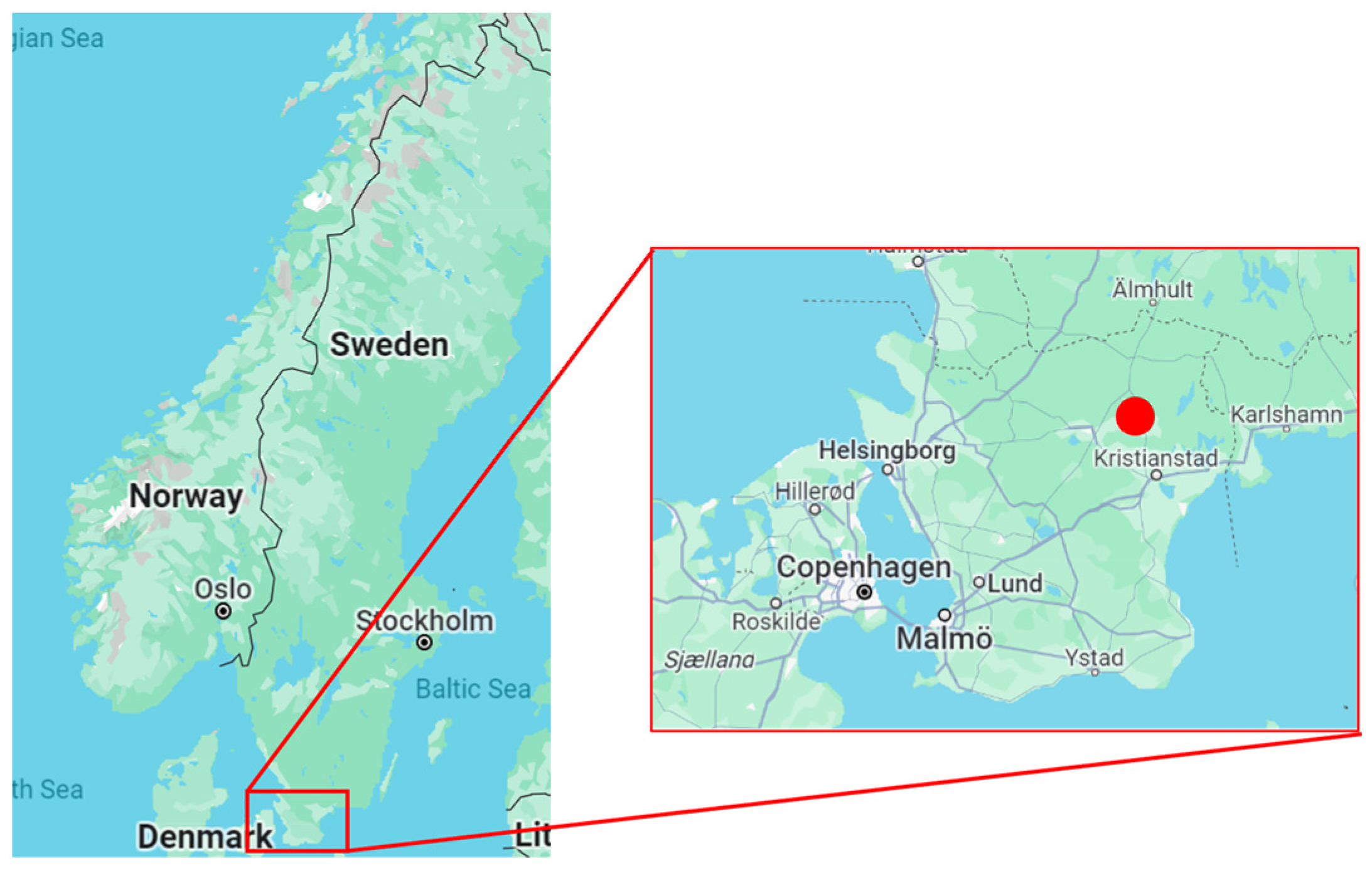
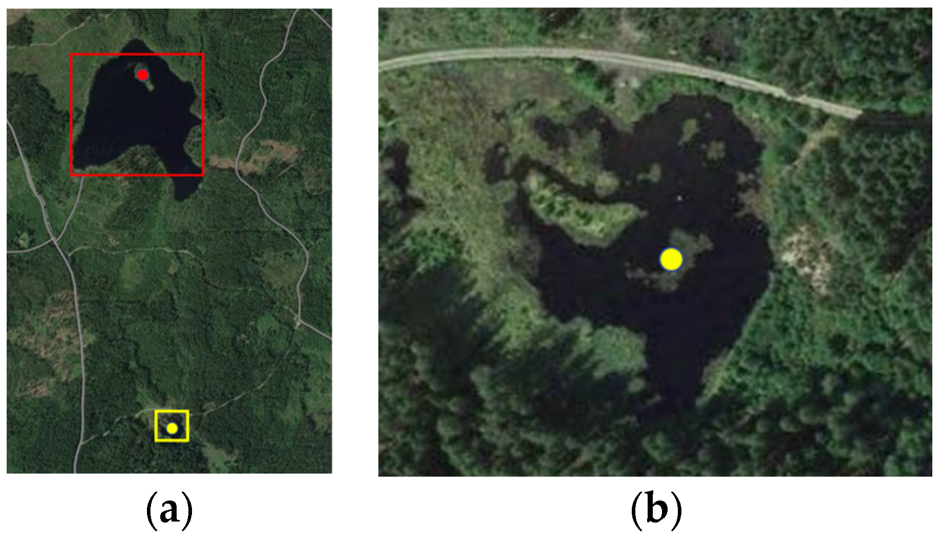
The studies in [32] were carried out in areas with smaller lakes and wetlands in north-eastern Scania, southern Sweden, Europe (marked as a red dot in Figure 1). More specifically, a smaller lake, Liasjön, which some mallards visited frequently, and a nearby wetland area (Figure 2a) were chosen with the core aim of studying how far wild and farmed mallards adapted to each other’s behavior.

A trap was set up in the wetland area of 100 by 100 m where the farmed mallards fed and also was important for sensor readings. Figure 2a shows the wetland area marked with a yellow frame indicating the wetland (extended in Figure 2b) and the lake, Liasjön, marked with a red frame. The distance between the yellow and red geolocated points was approximately 1000 m, with about 750 m between the lower red edge and the upper yellow edge.

The positions, in latitude and longitude, are shown in

Table 1. Liasjön, red marking the reference.

Place	Latitude	Longitude
Upper-left corner	56.45015	13.98744
Bottom-right corner	56.44700	13.99400
Reference point (red dot)	56.44950	13.99090

and

Table 2. The wetland, yellow marking the reference.

Place	Latitude	Longitude
Upper-left corner	56.44020	13.99180
Bottom-right corner	56.43950	13.99310
Reference point (yellow dot)	56.43983	13.99265

.

2.1. Preparatory Studies

The core result of the study material was stored in an Excel document with 19,916 data points. Information was originally received from the rings, identifying the mallards, and the attached GPS loggers (CatTraQ, Catnip Technologies, Ltd., Dallas, TX, USA), set to acquire position data once an hour. The data from the GPS loggers were downloaded with @trip PC (CatTraQ) and converted into .csv files and then further converted to an Excel document [32]. The Excel document and its columns showed the date, the time, the position, and the type of mallard (wild or farmed). The data were acquired during the period of August to October 2012 and, in some cases, also until November of the same year. The study obtained data from 56 individual mallards, of which 12 were wild mallards and 44 were farmed.

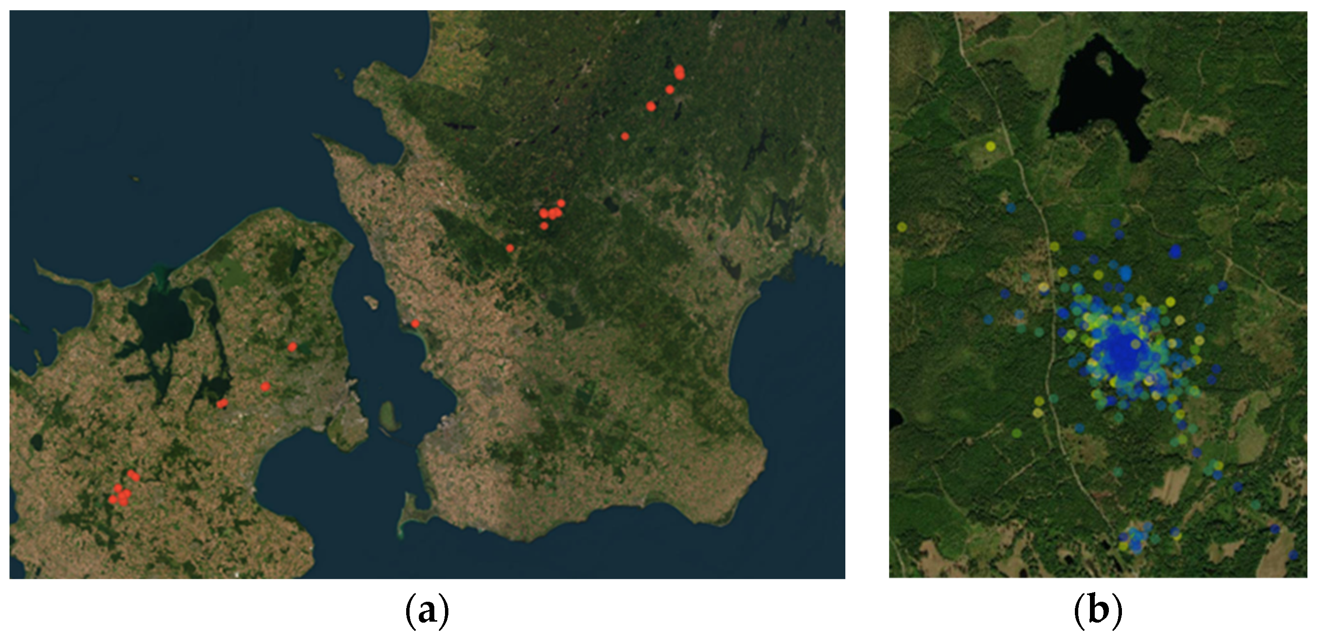
At a general level, it could be shown that there were differences in the movements with respect to the type of mallards: the wild mallards did move south-west during the later parts of the fall, while the farmed mallards hardly at all moved away from the wetland where they were brought up. Figure 3a,b illustrates the gap in behavior between the mallard types, showing that the two types of mallards could almost be interpreted as two different species.

This study focused on a limited time frame from 28 September 2012 to 2 October 2012 to be able to follow the complete movement patterns of a set of mallards. The results of this study will later be elaborated upon in future studies, scaling it up including aspects of behaviors besides movements.

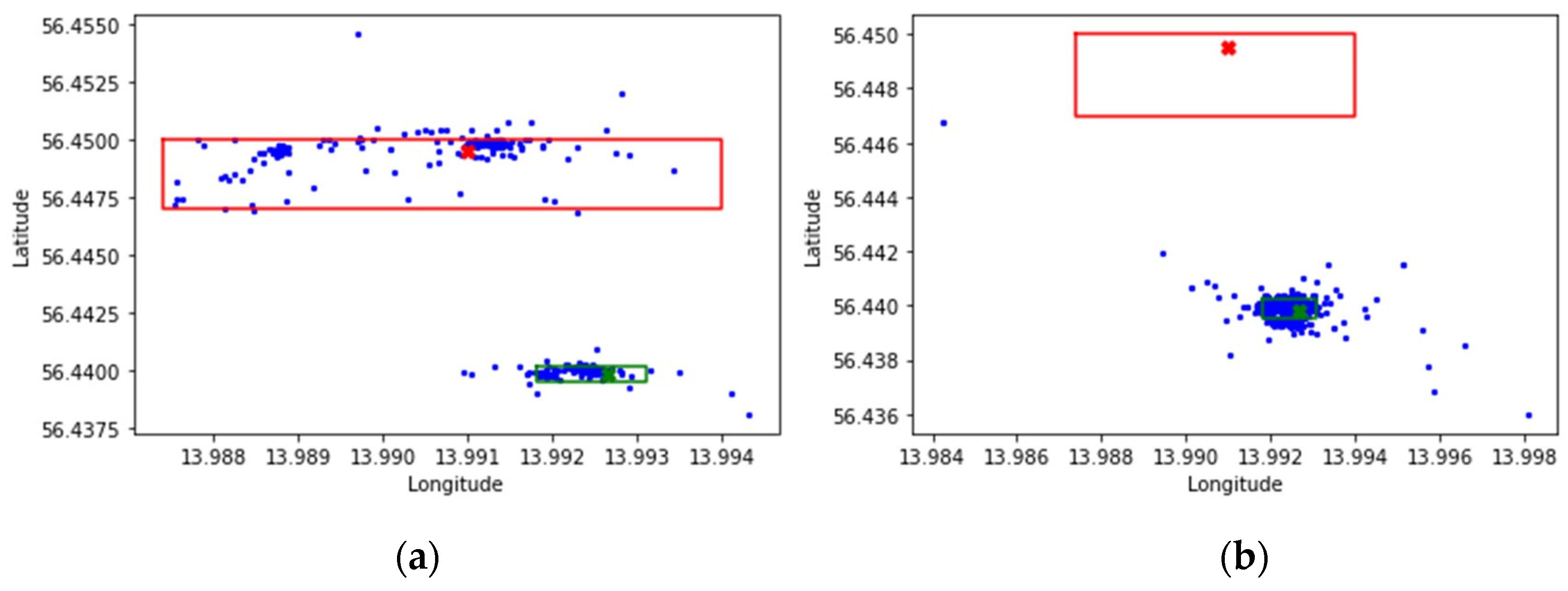
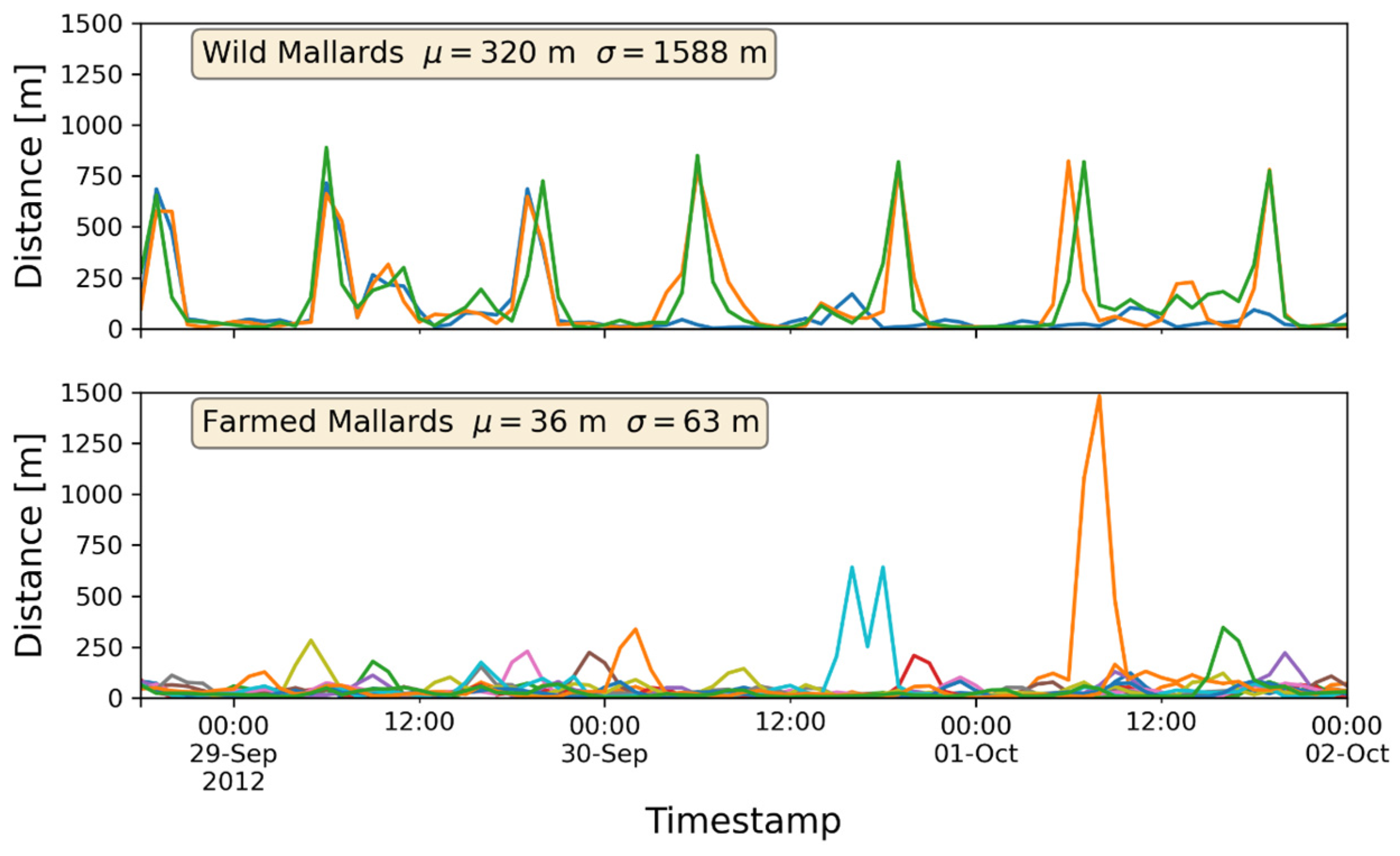
The narrowed dataset contained 1193 data points, including position, date, and time, where 415 data points reflected the movements of the wild mallards and 788 data points reflected the farmed ones. Differences in movements could clearly be seen on a more detailed level, as illustrated in Figure 4a,b.

Both scatterplots of Figure 4 correspond to the map of Figure 3a, including the colored reference points and frames. The yellow color, though, has been replaced by green for visibility reasons. Furthermore, Figure 4 illustrates the positions the mallards have taken at different times. The wild mallards seemed to have moved around in the areas of Liasjön as well as the wetland, while the farmed mallards mostly stayed in and around the wetland. More precisely, out of the 415 data points for the wild mallards, 167 points were within the frame of Liasjön and 191 points were within the wetland frame. Furthermore, 487 points out of 778 representing the farmed mallards were within the wetland area. The rest of the data points were close by the border of the wetland area, possibly also data points associated with water.

The study in [32] moreover showed that wild mallards are especially active during dawn and dusk. The farmed mallards, however, did not show this behavior at all. Figure 5 illustrates the wild mallards’ positions during nighttime and during daytime. Parts of the day, and here as night, dawn, day, and dusk, and the data points for those (source for time points for part of day, including dawn and dusk (in Swedish): Soluppgång och solnedgång Osby, August 2012 (https://www.sunrise-and-sunset.com/en (accessed on 28 January 2024))), were used to identify the significance of the movements. Due to daylight saving, the data were affected by shorter days in October in comparison to those in August. This is reflected in the scatterplots of the wild mallards’ positions during the daytime and nighttime, as illustrated in Figure 5a,b. It clearly shows the wild mallards fly between Liasjön and the wetland at dawn and dusk to spend their daytime at Liasjön and their nighttime at the wetland.

It can be concluded from the studies that approaching a model and simulating the mallards include several challenges, such as:

• The difference in behavior between the types of mallards.
• Imbalances in data points, with respect to:
  • Farmed versus wild mallards.
  • Data points representing swimming in the lake or wetland versus flying between such areas.
• On a timeline, the data points are quite sparse, one data point per hour making it rather difficult to predict the next exact data point based on the current data point or a set of previous points.

2.2. Time-Series Analysis—Overview

The mallard dataset contained a time series of several individual farmed and wild mallards. The dataset was treated as two subsets, corresponding to farmed and wild mallards. Each subset contained several different time series corresponding to the individual mallards. The prediction models were trained separately on the farmed and wild mallards. The model was the same for the two subsets, but the trained models differed because the model parameters were trained on two different data subsets.

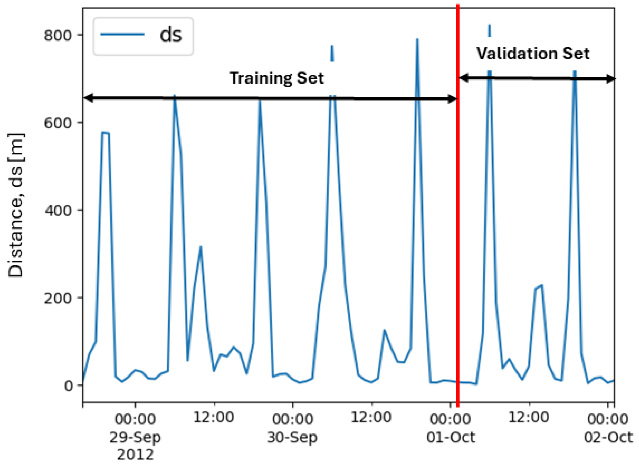
Two separate time-series analyses were conducted, one where the time series was divided into a training set and a validation set for each subset of mallards. The beginning of the time series was used as a training set, and the end of the time series was used as a validation set. The validation set consisted of 24 data points, and the training set consisted of 58 data points, leading to a 79% to 21% division of the training and validation sets. The validation set was chosen to be at least 24 h. Thus, we ended up with this division of the training and validation sets, as depicted in Figure 6.

Two different models were trained on the two different subsets of mallards. The difference between the models was in the feature set. The second model included a feature containing information regarding sunrise and sunset. In this analysis, only models predicting one value were investigated. An overview of this analysis is found in

Table 3. Overview of the different models, subsets, and validation set for the first time-series analysis. These models predict one value into the future. The predictive model excluding sunset in the table is depicted in Figure 9. The predictive model including sunset is depicted in Figure 10. The validation set consisted of 24 data points (corresponding to 29% of all data points), and the training set consisted of 58 data points (corresponding to 79% of all data points).

Model	Subset	Validation Set
Baseline	Farmed mallards	N/A
Baseline	Wild mallards	N/A
Predictive, excluding sunset	Farmed mallards	1 October 2012–2 October 2012
Predictive, excluding sunset	Wild mallards	1 October 2012–2 October 2012
Predictive, including sunset	Farmed mallards	1 October 2012–2 October 2012
Predictive, including sunset	Wild mallards	1 October 2012–2 October 2012

.

For the second analysis, a test set was added. One (1) time series, corresponding to one individual mallard, was excluded from the training and validation sets and was used as a separate test set, which is depicted in Figure 7.

This was performed separately for the wild and farmed mallard data subsets. In the second analysis, both prediction models that predicted 1 future value and models that predicted 12 future values were investigated. An overview of this analysis is found in

Table 4. Overview of the different models, subsets, and prediction length for the second time-series analysis. The second analysis included predictive models that used past values (12 h) for the prediction and models that did not. The analysis also used a test set with data from an individual mallard that was excluded from the training and validation sets.

Model	Subset	Future Prediction
Baseline	Farmed mallards	N/A
Baseline	Wild mallards	N/A
Predictive, no history	Farmed mallards	1 h and 12 h
Predictive, no history	Wild mallards	1 h and 12 h
Predictive, including history	Farmed mallards	1 h and 12 h
Predictive, including history	Wild mallards	1 h and 12 h

.

Several different neural network models were used in this paper, and an overview of these can be found in [33]. For all models, the Keras early stopping method [34] was used, where the monitored metric is the validation loss.

2.3. Preparations—Time-Series Analysis

The sample time was approximately 1 h. The different time series had different lengths, and there also were gaps in the time series. A gap was defined by a time difference of (over) 2 h between consecutive instances. Each gap resulted in the time series being divided, and in further analysis, it was treated as two separate time series. From the original 56 time series, it became 454 different time series. All time series shorter than 48 h were dropped, leaving 122 time series corresponding to 52 individual mallards, of which 10 were wild. The “cleaned” dataset contained 12,758 data points/instances.

The latitude and longitude were projected into flat x- and y-coordinates by an ellipsoid (WGS 84) [35] projection using the program package pyproj [36], thus giving the mallards’ position in meters on a flat plane. For each time series, the following consecutive differences between consecutive data points were calculated: time difference, sample time, and distance in the x-direction and the y-direction in meters. The derived quantities are shown in

Table 5. From the x- and y-coordinates, the relative distance was calculated in polar coordinates.

Timestamp (TS)	x-coord	y-coord	dx	dy	ds	θ	Diff TS
t0	x0	y0
t1	x1	y1	dx1 = x1 − x0	dy1 = y1 − y0	ds1	θ1	dt1 = t1 − t0
t2	x2	y2	dx1 = x1 − x0	dy1 = y1 − y0	ds2	θ2	dt2 = t2 − t1

.

The distance (ds) between consecutive data points was calculated as the Euclidian distance derived from the difference in the x- and y-directions for each consecutive data point, i.e.,

$$ds=\sqrt{{dx}^2+{dy}^2}.$$

(1)

The direction ($\theta$) was calculated as the angle defined by the positive x- and y-directions, i.e.,

$$\theta ={\tan }^{-1}\frac{dy}{dx}.$$

(2)

The distance was interpolated so that an exact sample time of 1 h was achieved.

2.4. First Approach of Prediction of Movement Patterns—Time-Series Analysis

Welch’s t-test was conducted with the null hypothesis being that wild mallards and farmed mallards move the same average distance. Additionally, a visual inspection of the mallard movements was performed, comparing the two types. This Welch’s t-test motivated the approach for treating the two types of mallards in the subsequent time-series analysis.

The time-series analysis was limited to the period from 28 September 2012 at 16:00 to 2 October 2012 at 01:00. Within this time frame, seventeen different time series were extracted from the original dataset. Three of these time series pertained to wild mallards, while the remaining fourteen were related to farmed mallards. The data for the mallards were divided into two sets: a training set and a validation set. The training set covered the period from 28 September 2012 at 16:00 to 1 October 2012 at 01:00, and the validation set spanned from 1 October 2012 at 02:00 to 2 October 2012 at 01:00. Throughout the analysis, the mean absolute error (MAE) was used as the regression metric.

$$MAE=\frac{1}{n}\sum _{k=1}^n\left|y_{true}^{\left(k\right)}-y_{pred}^{\left(k\right)}\right|$$

(3)

was used consistently during the prediction analysis. The mean absolute error (MAE) metric was chosen over the more commonly used root mean square error (RMSE) for this analysis. The RMSE’s quadratic behavior tends to give higher weight to larger differences, which could be problematic, given that mallards, particularly wild ones, often move significantly longer distances twice a day. Using the MAE metric helped to mitigate the disproportionate impact of these longer movements on the model’s training. The MAE metric was used for comparison between the different predictive models and also for comparison with the baseline models mentioned later.

Two baseline models were implemented for comparison with the prediction models. The first, named “last”, used the most recent observed value for prediction. The second, called “12 h-repeat”, used the value from 12 h prior. Both models were evaluated using the same validation set and sequence length as the predictive neural network (NN) models. The study involved two neural network models, as shown in Figures 9 and 10, which were trained on two different subsets of data—one for wild mallards and the other for farmed mallards—with MAE calculations for both. After evaluating performance with three types of recurrent neural networks (SimpleRNN [37], gated recurrent units (GRUs), and long short-term memory (LSTM)), the LSTM neural network was selected for a more in-depth grid search due to its marginally lower error rates.

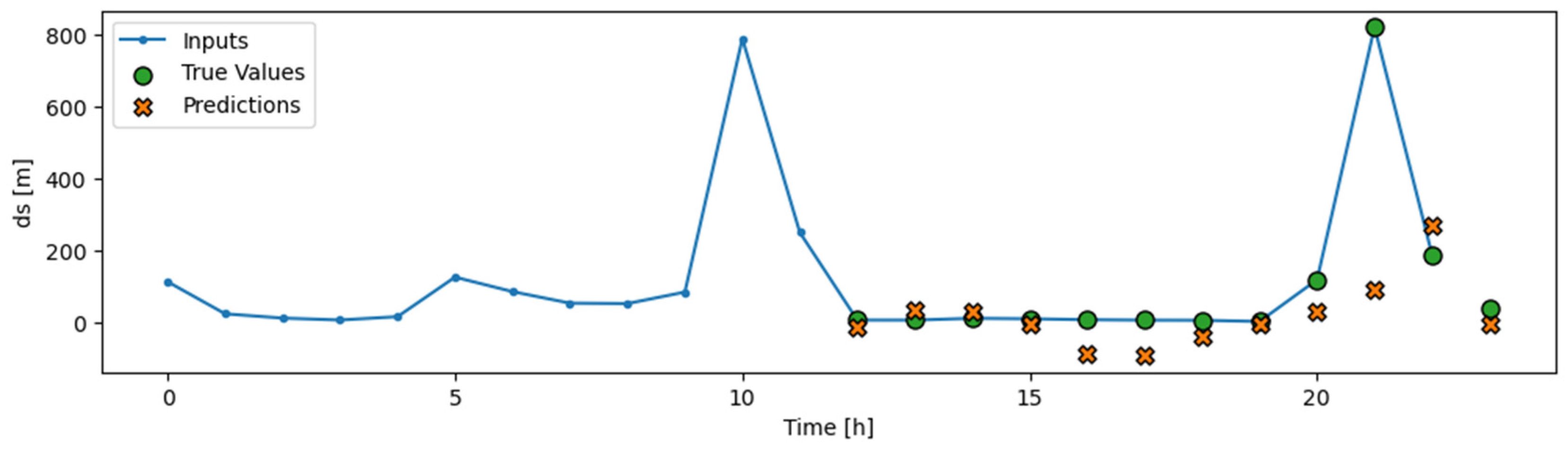
The data for these models were segmented into rolling windows of 6, 12, and 24 samples (each sample representing an hour), and the networks were tasked with predicting the mallards’ movements for the subsequent hour. An illustration of this prediction model is presented in Figure 8, where actual values are marked as green circles and predicted values as red Xs.

The neural network models tested varied in complexity, with configurations of 1, 2, or 3 layers. Each layer consisted of 24, 32, or 48 neurons. This range of configurations led to a total of 27 different simulations for both wild and farmed mallards.

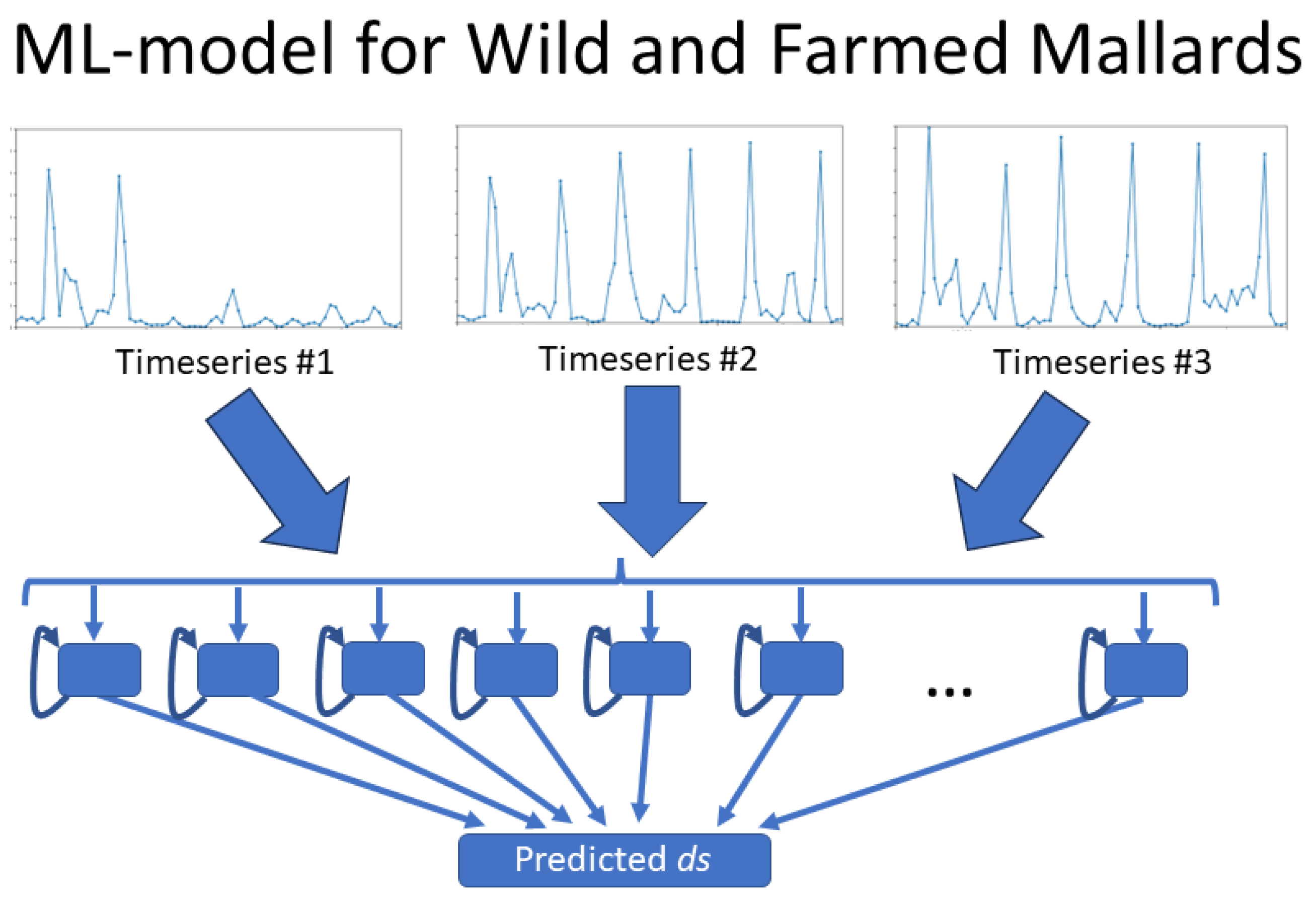
For the wild mallards, three individual time series—each corresponding to a different mallard—were used as input for the neural network, as illustrated in Figure 9. The network’s output was the averaged mean absolute error (MAE) calculated from the predicted time series for these three inputs.

In the case of farmed mallards, fourteen time series were available. Out of these, twelve were selected for training the network. These twelve time series were further divided into four subsets, with each subset containing three time series. The neural network was trained separately on each subset. The output for each subset was the average of the MAE values from the three time series, similar to the approach for wild mallards. These four averaged MAE values were then combined to produce a final averaged MAE value for the farmed mallards.

This methodology was chosen to maintain identical model structures in terms of the number of parameters for both wild and farmed mallards, thereby facilitating a more accurate comparison of the results between the two types of mallards.

A second set of predictions was conducted, identical to the first set but with an additional feature referred to as “part of day data”. This feature incorporated information about the time of day for each sample in the time series, categorizing it into dawn, day, dusk, or night (as depicted in Figure 10). Consequently, for the wild mallards’ dataset, the input for the neural network comprised four features: the three time series corresponding to the individual mallards and a fourth series indicating the part of the day to which each data point belonged.

The dataset for farmed mallards, which included fourteen time series, was processed in a manner similar to ML-model I, as described before. The key distinction in this approach was the incorporation of an additional feature, “part of day data”. This feature was integrated into the model, augmenting the existing dataset with information about the time of day for each data.

2.5. Second Approach of Prediction of Movement Patterns—Time-Series Analysis

In the second approach to time-series prediction, a test set was incorporated. The existing training set was further divided into a pure training set and a validation set, maintaining the same division as in the previous analysis case. The notable change involved the treatment of wild mallards’ data: the model was trained using two of the mallards, while the third served as a test set encompassing the complete time series from 28 September 2012 at 16:00 to 2 October 2012 at 01:00. This procedure was applied to each of the three wild mallards, effectively acting as a form of cross-validation. For the farmed mallards, one time series was designated as the test set and the other thirteen as the training and validation sets. This selection was randomly made for three mallards from the farmed mallard dataset.

This second approach enabled both single-step and twelve-step predictions. An illustration of the twelve-step prediction, using a sliding window of 12 data samples (equivalent to 12 h), is presented in Figure 11.

In this second approach, a test set from a different mallard was used to measure performance, contrasting with the first approach.

Table 6. The different models used for the one-hour and twelve-hour predictions. The linear model was implemented using the Keras dense class but without an activation function.

Model	Hyperparameters	Used in 1 h Prediction	Used in 12 h Prediction
Last	N/A	Yes	Yes
12 h repeat	N/A	No	Yes
Linear	N/A	Yes	Yes
Dense	32 + 32 neurons	Yes	No
Dense	64 neurons	No	Yes
CNN	32 filters	Yes	Yes
LSTM	32 + 32 neurons	Yes	Yes
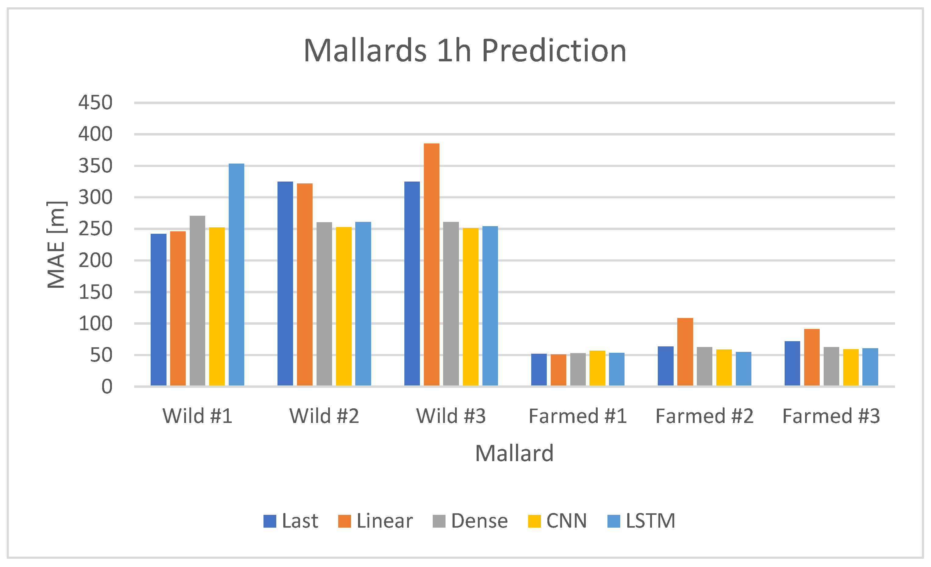
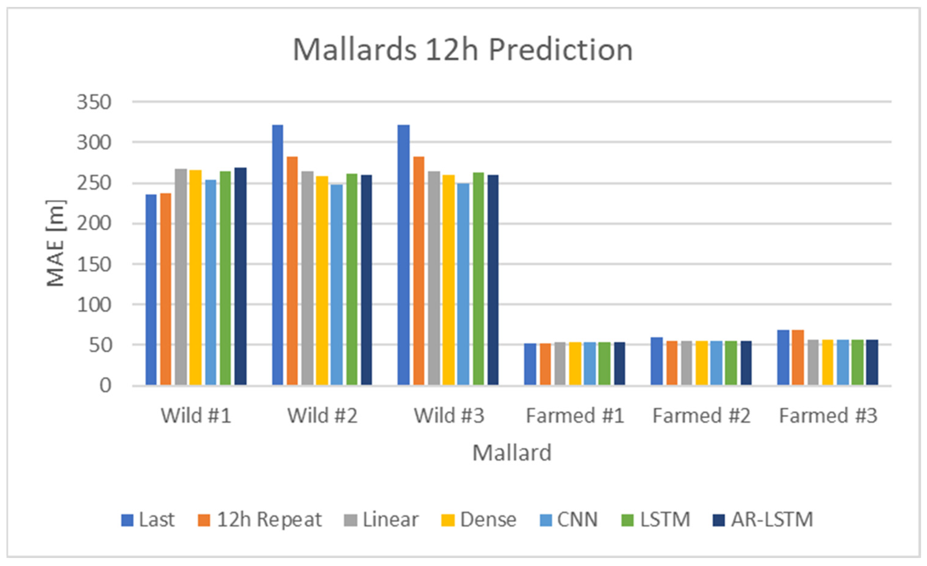
AR-LSTM	32 + 32 neurons	No	Yes

displays the various models along with their respective hyperparameters. Additional hyperparameter values were tested, but these did not result in significant changes. The primary objective of this study was to determine whether any model could outperform the baseline models “last” or “12-h repeat”.

The baseline or naive models either used the last observed value for prediction or repeated the last 12 values. In contrast, the linear and dense models made predictions about future values based solely on the present value. The convolutional neural network (CNN) and LSTM models, however, based their future value predictions on the past twelve values. The AutoRegressive (AR)-LSTM model operated differently, making predictions in 1 h increments. These predictions were recursively fed back into the model, allowing it to make subsequent predictions conditioned on the previous one. This process was repeated 12 times, enabling the model to forecast up to 12 h into the future. For a comprehensive view of the different models used in this analysis, see Table 6.

The linear model was implemented using the Keras dense class [38] but without an activation function. The dense models were also implemented with the Keras dense class but with the rectified linear unit (relu) activation function. The relu activation function was also used in the CNN model.

3. Results

3.1. Different Movement Patterns between Wild and Farmed Mallards

The Welch t-test analysis revealed a statistically significant difference between the movement patterns of wild and farmed mallards. Wild mallards, with an average movement distance of 320 m (standard deviation, σ = 1588 m), traveled nearly nine times farther on average compared to farmed mallards, who had an average movement of 36 m (σ = 63 m). This difference was statistically significant, with a p-value of less than 0.001. Additionally, the variance in the distance moved by wild mallards was substantially larger than that for farmed mallards.

The Welch t-test results further confirmed the distinct movement patterns of wild and farmed mallards. The test showed that wild mallards, on average, moved almost nine times further between samples compared to farmed ones. This significant difference, demonstrated through the two-sample Welch t-test with non-overlapping results, underlined the need for separate prediction models for each subgroup of mallards.

Regarding their direction, the distribution for both types of mallards was nearly uniform, indicating a tendency to move in random directions. This finding suggests that distinct simulation or internal models are necessary to accurately represent the movements of farmed and wild mallards separately. The distinct movement patterns of the two types of mallards are illustrated in Figure 12.

3.2. First Approach of Movement Predictions—Time-Series Analysis

For both subsets of mallards—the farmed and the wild—the analysis demonstrated improved results compared to the naive model. These results are detailed in

Table 7. The MAE for wild mallards for different layer sizes and number of layers.

Model	Layer Size	“Part of Day” Feature Included	MAE
1-layer LSTM	48 neurons	No	26 m
2-layer LSTM	24 + 24 neurons	Yes	32 m
3-layer LSTM	32 + 32 + 32 neurons	Yes	37 m
12 h repeat			95 m

and

Table 8. The MAE for farmed mallards for different layer sizes and number of layers.

Model	Layer Size	“Part of Day” Feature Included	MAE
1-layer LSTM	32 neurons	No	14 m
2-layer LSTM	24 + 24 neurons	No	18 m
3-layer LSTM	48 + 48 + 48 neurons	Yes	16 m
Last			28 m

.

Table 7 and Table 8 clearly demonstrate that the neural network models, specifically those using long short-term memory (LSTM) architecture, achieved a lower mean absolute error (MAE) for both wild and farmed mallards. The improvement factor in the MAE was approximately 4 for wild mallards and 2 for farmed mallards, indicating a significant enhancement in predictive accuracy for both types of mallards with these LSTM models.

3.3. Second Approach of Movement Predictions—Time-Series Analysis

Figure 13 presents the MAE values from the 1 h predictions for both wild and farmed mallards. Interestingly, these values were quite similar when comparing the baseline “last” model and the best predictive model for each group. However, the results did show variation among individual mallards. Specifically, for individuals labeled wild #2 and wild #3, the predictive models outperformed the baseline model. It is important to note that the MAE values for wild and farmed mallards were not directly comparable, as wild mallards generally moved more, leading to higher mean values in their time series.

Turning to the 12 h predictions, as shown in Figure 14, the outcomes were akin to the 1 h predictions. There was no significant difference between the performance of the baseline models and the predictive models across the board. However, similar to the 1 h predictions, this pattern did not hold consistently for all individual mallards.

4. Discussion

Machine learning (ML), as a technique to represent and draw conclusions from using large datasets, has increased use in various disciplinary fields. Using ML models simulating activities brings additional benefits as a platform for experimenting with different circumstances, such as tests of “what if” a specific event happens, what the outcome will be, or what the reaction will be from this.

While several approaches in animal behavior studies also using ML models have proven to be successful, this study highlights cases of using ML models simulating activities providing additional benefits. This shows possibilities supplementing insights in the absence of data (such as in cases of sensor failures) and serving as a platform for testing severe challenges in using ML techniques in a consistent manner. Large disparities in groups of data, in addition to individual deviations, have proven difficult to capture in a uniform ML model. These studies have observed large contrasts in movement patterns between wild and farmed mallards in selected areas of southern Sweden. Such contrasts, as well as imbalances in data representing such groups of mallards, here lead to conclusions introducing different ML models, depending on the type of mallard. This is of great importance as possible future approaches can address flock behavior through so-called multi-agent systems. Credible representations of flock behavior within a species need a clear dependency relationship to the type of animal within the species (here, wild or farmed mallard).

The study carried out in this contribution was based on [32], where differences in movement patterns between farmed and wild ducks were established. This study further contributed with more in-depth research into how the two mallard groups were contrasted to one another. The main purpose of this contribution was to investigate possibilities to reproduce simulations of mallard movement patterns with ML methods. With this done, more detailed information can be obtained through both ML simulations performed and the preparatory investigations of the data material that is needed to precede reliable ML models.

In addition, and as a conclusion, existing data material with the use of ML models allows ML-based simulation opportunities, which contribute to estimating behaviors lying outside the dataset. Such estimates can be used to forecast future behavior or to supplement with simulated data where actual data are missing, such as when sensors for periods provide insufficient or no data.

Adding sunrise or sunset information to the neural network model does not enhance predictions for either wild or farmed mallards. This is because for wild mallards, sunrise and sunset patterns are already implicit in their movement, as illustrated in Figure 10’s upper graph for two mallards. Similarly, farmed mallards show no significant movement changes during these times, explaining the lack of impact on predictions for them.

Comparative analysis of baseline (naive) models and LSTM neural networks for both wild and farmed mallards revealed that the recurrent neural networks offered superior predictions, with a considerably lower MAE compared to the baseline models. However, caution is advised due to the small size of the dataset relative to the number of neural network parameters, namely the weights.

The models demonstrated effective predictions when the same dataset for the mallards was used for both training and validation. This approach involved training the models on the same subjects, specifically three wild mallards and fourteen farmed ones. The validation then used the same individuals but used a different segment of the time series, taken from a later period.

In the second approach, where an individual from each group—wild and farmed—was excluded and used as a test set, the predictive models no longer yielded favorable results. This variation could be attributed to the unique movement patterns of each individual. For instance, as depicted in the upper part of Figure 9, not all wild mallards exhibited identical movement patterns. The models tended to predict an average movement for the two distinct groups—wild and farmed mallards—which did not accurately represent individual movements. The predictive model lost much of its accuracy, failing to outperform (naive) models, with similar MAE values for both predictive models and baseline models. This decrease in accuracy was understandable when considering the individual movement patterns within each group. Since each mallard exhibits a distinct behavior, it is challenging to develop a singular model for each group. A prospective method might involve modeling each mallard as an individual agent interacting with others.

Comparing the two approaches mentioned before, one sees that the first approach, in which all mallards of a respective type, farmed or wild, were used in the training set, the performance of the predictive models was significantly better compared to when a mallard of a respective type was left from both the training set and the validation set. In the first approach, the dataset was divided into a training set (79%) and a validation set (21%). But for the second approach, one mallard was left out and the corresponding data points, which were 33% of all data points in the case of wild mallards, considerably limited the size of the training set. This limitation of the training set and the overall small dataset, together with different individual movements between individuals, are the reason the performance of the second approach was not as good as that of the first approach.

One aim behind the study of this paper was to lay a foundation for further studies. While the work itself has shown interesting results, the models developed to represent individual birds will be extrapolated toward multi-agent systems to represent flocks of birds. The focus may also shift from the mallards studied here to geese, as described previously, with behavior also beyond pure movements and with the aim of serving as an experimental base for further knowledge of geese in changing environments.

5. Conclusions

Large amounts of data collected via sensors can advantageously form a basis for studies of animal behavior over a period of time. The collected data reflect the actual activities that took place during the time when the sensors were attached to the animals under study. This study addressed values of simulation models, where machine learning (ML)-based models were proposed and investigated. ML models were pointed out to contribute further with studies outside the dataset to, for instance, fill in gaps of missing data or predict the consequences of unforeseen events.

However, to draw valuable conclusions or to make valuable predictions, machine learning algorithms are normally in need of consistent and balanced datasets. A case was shown here where this was not the case. Therefore, the ML models were trained on different subsets of the whole dataset, one for each type of mallard. Thus, one ended up with an ML model of the same structure but with a different parameter set. That is, the structure of the ML model was the same for the two types of mallards in the comparison but the trained ML model was different. It was shown that this more nuanced way of using ML also contributed to more reasonable simulation models. In the case of this study, we had two groups of mallards, wild and farmed, and the behaviors of these two groups are significantly distinct.

A division of the ML models will form a basis for later studies when flock behaviors are simulated through the so-called multi-agent system and where a uniform ML model probably cannot function as a credible and efficient simulation model. The results from these studies will point to a possible strategy for representing several different animal species simultaneously using ML. ML has generally shown great potential in animal behavior studies, but as behaviors between animal groups differ greatly, it is reasonable to apply different ML models per animal group rather than striving for a uniform comprehensive one.

Experiments were conducted with several different types of ML algorithms to investigate differences in performance between them. The experiments showed that the recurrent neural network is the algorithm that shows the greatest performance when all mallards of one type are used in the training set. Removing one individual mallard from the training set and then using the trained model on this new dataset does not work that well, which was discussed in the previous section. In further studies, it is this algorithm that is primarily recommended.