Detecting IoT Anomalies Using Fuzzy Subspace Clustering Algorithms

Abstract

There are many applications of anomaly detection in the Internet of Things domain. IoT technology consists of a large number of interconnecting digital devices not only generating huge data continuously but also making real-time computations. Since IoT devices are highly exposed due to the Internet, they frequently meet with the challenges of illegitimate access in the form of intrusions, anomalies, fraud, etc. Identifying these illegitimate accesses can be an exciting research problem. In numerous applications, either fuzzy clustering or rough set theory or both have been successfully employed. As the data generated in IoT domains are high-dimensional, the clustering methods used for lower-dimensional data cannot be efficiently applied. Also, very few methods were proposed for such applications until today with limited efficacies. So, there is a need to address the problem. In this article, mixed approaches consisting of nano topology and fuzzy clustering techniques have been proposed for anomaly detection in the IoT domain. The methods first use nano topology of rough set theory to generate CORE as a subspace and then employ a couple of well-known fuzzy clustering techniques on it for the detection of anomalies. As the anomalies are detected in the lower dimensional space, and fuzzy clustering algorithms are involved in the methods, the performances of the proposed approaches improve comparatively. The effectiveness of the methods is evaluated using time-complexity analysis and experimental studies with a synthetic dataset and a real-life dataset. Experimentally, it has been found that the proposed approaches outperform the traditional fuzzy clustering algorithms in terms of detection rates, accuracy rates, false alarm rates and computation times. Furthermore, nano topological and common Mahalanobis distance-based fuzzy c-means algorithm (NT-CM-FCM) is the best among all traditional or nano topology-based algorithms, as it has accuracy rates of 84.02% and 83.21%, detection rates of 80.54% and 75.37%, and false alarm rates of 7.89% and 9.09% with the KDDCup’99 dataset and Kitsune Network Attack Dataset, respectively.

1. Introduction

There are huge applications comprising sensors providing critical data that evolve mostly as a result of the development of the IoT [1] along with their sources of real data generation. As a result, a rapid surge in streaming and time-series data availability is witnessed. Analyzing such data can yield insightful information.

The uncovering of anomalies from IoT data has substantial real-world applications across various activities such as pre-emptive maintenance, prevention of fraud, fault finding, and monitoring. Therefore, detecting anomalies can provide actionable information in the circumstances, where no trustworthy answers exist. A reliable answer to the problems is put forwarded here.

High dimensionality typically makes difficult-to-discover anomalies in an IoT dataset. Data sparsity is a result of the fact that as the features or attributes grow, more data are necessary for the generalization of the detection system. These extra variables, or a significant quantity of noise from numerous insignificant features hiding the genuine outliers, are the cause of the data sparsity. The “curse of dimensionality” [2,3] is a famous term coined for the problem. Therefore, several conventional anomaly detection techniques like k-means, k-medoids, and DBSCAN [4,5,6] were found to be unsuitable for such data as they fail to retain their efficacy. Efficient anomaly detection of high-dimensional IoT data is an interesting problem of research.

In [7], the authors introduced a new concept called rough set theory, for dealing with uncertainty or vagueness existing in any real-life problem. In [8], a classification algorithm based on a neighborhood rough set was proposed for the anomaly detection in mixed-attribute datasets. In [9], the authors defined the nano topological space of a subset X of universe U using both of the approximations of X. In [10], the authors proposed to generate CORE (a subset of attribute sets) of the conditional attribute set for medical diagnosis. The method in [9] can be used to address the “curse of dimensionality” problem that exists in high-dimensional IoT data.

Clustering is a data mining technique used to unearth the distribution of data and the patterns in any dataset. Clustering has been widely applied in anomaly detection. In [11], the authors used the k-means algorithm for anomaly detection in a network-traffic dataset. A fuzzy c-means clustering-based technique for anomaly detection in mixed data had been put out by the authors in [12]. In [13], the authors put forwarded a hierarchical clustering method for mixed-data anomaly detection. For detecting anomalies in mixed data, in [14], a hybrid clustering strategy was proposed that combines both partitioning and hierarchical techniques. In [15], a method of finding anomalies in high-dimensional and categorical data was proposed. Analogous research was presented in [16,17,18,19,20,21,22,23,24,25,26,27,28,29]. The authors of [30] addressed the insider threat, which poses serious problems for the industrial control systems’ cyber security. The authors of [31] presented an online random forest-based anomaly detection method. In [32,33,34], fuzzy techniques for real-time anomaly detections were covered. For the purpose of identifying anomalies in significant cyberattacks, the authors of [35] presented a neural network-based fuzzy approach.

The majority of the aforementioned algorithms have some limitations. Some, for instance, are ineffective in finding anomalies in high-dimensional data, while others lose detection accuracy with the increase in dimensions. In [36], the authors put forwarded a mixed algorithm consisting of a partitioning and a hierarchical approach for real-time anomaly detection which produces stable clusters along their fuzzy lifetimes. However, this approach loses efficacy when the dimension of the dataset increases. Also, the traditional k-means algorithm has a wide range of applications, but it is not free from difficulties such as difficulties in determining the number of clusters, sensitivity to initial cluster-centers, low accuracy rate, etc. Some of the aforesaid issues were addressed nicely in [14,36,37,38,39,40] up to some extent. But there is still room for improvement.

Anomaly detection models based on the fuzzy c-means clustering algorithm [32,41,42,43,44,45,46,47] can be a better solution for the aforesaid issues for three primary reasons. Firstly, fuzzy clustering allows for the overlapping of clusters useful in dealing with the complex structure or ambiguity or overlapping class boundaries available in the datasets. Secondly, they are more robust to the anomalies and noise, as the transition from one cluster to another is gradual. Thirdly, because it enables a more thorough depiction of the relationship between data points and clusters, fuzzy clustering offers a more nuanced view of the data’s structure. In [48], the authors proposed a new algorithm, MSRFCM (Mahalanobis Shadowed Rough Fuzzy Clustering Method), which uses Mahalanobis distance to improve the accuracy of intrusion detection. Using the principal component analysis for selecting most discriminative features, a fuzzy c-means clustering approach was presented in [41] for intrusion detection in network data. In any IoT application, the data are high-dimensional. Also, the computation of high-dimensional correlation matrices for Mahalanobis distance is almost impossible, so it does not work well for high-dimensional data.

In this article, most of the shortcomings of all of the aforesaid methods are addressed in an efficient manner, and some hybrid approaches are proposed which use nano topology and a couple of fuzzy clustering algorithms for the efficient detection of anomalies in high dimensional IoT data.

This paper’s objective is described as follows:

• A nano topology [9,49] along with its basis is constructed to identify a subspace using the Nano Topology-based Subspace Generation Algorithm.
• Secondly, a couple of well-known fuzzy clustering approaches are proposed to generate soft clusters.
• A comparative analysis is conducted among all of the proposed approaches along with the traditional fuzzy clustering approaches.

The methods initially find a smaller dimensional space by deleting unnecessary features using a rough set theoretical approach. Then, fuzzy clustering-based approaches, namely the fuzzy c-means algorithm (FCM) [41,47], Gustafson–Kessel Algorithm (GK) [42,43,44,45,46,47], Gath–Geva Algorithm (GG) [43,47], Mahalanobis Distance-based Fuzzy c-Means algorithm (M-FCM) [47], and Common Mahalanobis Distance-based Fuzzy c-Means algorithm (CM-FCM) [47], are used on it to identify the fuzzy clusters. The approaches time complexities are also calculated. The proposed approaches are then tested with the help of MATLAB and the datasets KDDCup’99 [50] and Kitsune Network Attack Dataset [51] (https://github.com/ymirsky/Kitsune-py (accessed on 12 December 2021)), and comparisons are also made. The results convincingly show that the nano topology-based approaches outperform the traditional fuzzy clustering approaches in many parameters, and the nano topology-based CM-FCM (NT-CM-FCM) is the most efficient one.

The paper is prescribed in the following manner. The problem statement is presented in Section 2. The proposed methods are discussed in Section 3. The complexity analysis of the methods is presented in Section 4. The experimental results and discussions are presented in Section 5, and the paper’s conclusions, limitations, and recommendations for further research are presented in Section 6.

2. Problem Statement

Below, some vital terms and definitions from [9,10,49] used in this paper are described.

2.1. Definition 2.1 [49]

A set-valued information system [49] is given by quadruple S = (X, A, V, f), where X is a non-empty finite set of IoT data instances, A is a finite set of attributes, V = ∪V_a, where V_a is a domain of the attribute a ∈ A. We define f: X × A → P (V), such that ∀x ∈ X and a ∈ A, f (x, a) ∈ V_a and f (x, a) $\ge$ 1. Also, A = {C ∪ {d}; C ∩ {d} = ϕ}, where C is the conditional attributes, and d is the decision attribute.

2.2. Definition 2.2 [49]

If the domain of a conditional attribute of IoT data can be arranged in ascending or descending order of preferences, then such an attribute is called the criterion. If every conditional attribute is a criterion, then the information system is known as a set-valued ordered information system [49].

2.3. Definition 2.3 [49]

If the values of some IoT data instance in X under a conditional attribute can be ordered according to the inclusion of increasing or decreasing preferences, then the attribute is an inclusion criterion [49].

2.4. Definition 2.4 [49]

Let us consider a set-valued ordered information system with an inclusion increasing preference. Also let $R_A^{\ge }$ be a relation defined as

$$R_A^{\ge }=\left\{\left(y,x\right)\in X\times X:f\left(y,a\right)\ge f\left(x,a\right)\forall a\in A\right\}$$

(1)

$R_A^{\ge }$ is said to be the dominance relation on X, when ${(y, x)\in R}_A^{\ge },$ then $y{\ge }_{A}x$, which means that y is at least as good as x with respect to A.

2.5. Property 1 [9,49]

The inclusion dominance relation $R_A^{\ge }$ is (i) reflexive, (ii) unsymmetric, and (iii) transitive.

2.6. Definition 2.5 [9,49]

For x ∈ X, the dominance class of x is given by

$$[{x]}_A^{\ge }=\{yϵX:\left(y, x\right)ϵR_A^{\ge }\}=\{yϵX:f\left(y, a\right)\ge f\left(x,a\right), \forall a ϵ U\}$$

(2)

where $X_A^{\ge }=\{{\left[x\right]}_A^{\ge }:x ϵ X\}$ is the family of dominance classes.

2.7. Remark 1 [9,49]

$X_A^{\ge }$ is not a partition of X but induces a covering of X, that is X = ∪$[{x]}_A^{\ge }$.

2.8. Definition 2.6 [9,49]

Given a set-valued ordered information system S = {X, A, V, f} and a subset B of X, the upper approximation and lower approximation of B are, respectively, given by

$${UP}_A^{\ge }\left(B\right)=\left\{xϵX:{\left[x\right]}_A^{\ge }\cap B\ne \varphi \right\}$$

(3)

and

$${LO}_A^{\ge }\left(B\right)=\{xϵX:[{x]}_A^{\ge } \subseteq B\}$$

(4)

Also, the boundary region of X is given by

$${BD}_A^{\ge }\left(B\right)={UP}_A^{\ge }\left(B\right)-{LO}_A^{\ge }\left(B\right)$$

(5)

2.9. Definition 2.7 [9,49]

Given a set-valued ordered information system S, a subset D of A is said to be a criterion reduction of S if $R_A^{\ge }=R_D^{\ge }$ and $R_M^{\ge }\ne R_A^{\ge }$ for any M ⊆ D. In other words, a criterion reduction of S is a minimal attribute set D such that $R_A^{\ge }=R_D^{\ge }$.

2.10. Definition 2.8

$$\mathrm{CORE} (A) \mathrm{is} \mathrm{given} \mathrm{by} \mathrm{CORE} (A)=\{aϵA:R_A^{\ge }\ne R_{A-\left\{a\right\}}^{\ge }\}$$

(6)

[see, e.g., [9,49]].

2.11. Definition 2.9 [9,49]

Let $R_C^{\ge }$ be a dominance relation on X, then ${\tau }_C^{\ge }\left(B\right)=\{X,\varphi ,{UP}_C^{\ge }\left(B\right),{LO}_C^{\ge }\left(B\right),{BD}_C^{\ge }\left(B\right)\}$ forms a nano topology [10,49] on X with respect to B. And ${\beta }_C^{\ge }\left(B\right)=\{X,{UP}_C^{\ge }\left(B\right),{LO}_C^{\ge }\left(B\right)\}$ is the basis for ${\tau }_C^{\ge }\left(B\right)$. Furthermore, CORE (C) = $\{aϵC:{\beta }_C^{\ge }\ne {\beta }_{C-\left\{a\right\}}^{\ge }\}$ = $\cap$ red (C), where red (C) denotes the criterion reduction.

2.12. Definition 2.10 [9,49]

Let S = (X, A, V, f) be an information system consisting of m entities or objects x₁, x₂,…, x_m. Let the attribute set A have n members. Then, S can be viewed as a m × n matrix in which rows represent objects and columns represent attributes. Attributes can be termed as features or dimensions.

2.13. Definition 2.11

Each IoT data instance consists of n measured variables grouped into an n-dimensional vector x_i = [x_i1, x_i2,…, x_in], x_i ∈ Rⁿ. A set of N data instances is given by X = {x_i; i = 1, 2,…, N} and is expressed as an N × n matrix as follows:

$$\mathit{X}=\left[\begin{array}{c}\begin{array}{ccc}{\mathit{x}}_{\mathbf{11}}& {\mathit{x}}_{\mathbf{12}}& \dots {\mathit{x}}_{\mathbf{1}\mathit{n}}\\ {\mathit{x}}_{\mathbf{21}}& {\mathit{x}}_{\mathbf{22}}& \dots {\mathit{x}}_{\mathbf{2}\mathit{n}}\\ \dots & \dots & \dots \dots \end{array}\\ {\mathit{x}}_{\mathit{N}\mathbf{1}} {\mathit{x}}_{\mathit{N}\mathbf{2}} \dots {\mathit{x}}_{\mathit{N}\mathit{n}}\end{array}\right]$$

(7)

The fuzzy clustering is the finding of the fuzzy partitioning space for X and is expressed by the following matrix.

$$F_{\mathrm{fc}}=\{[{\mathsf{\mu }}_{\mathrm{ij}}{]}_{\mathrm{c}\times \mathrm{n}}; {\mathsf{\mu }}_{\mathrm{ij}}\in [0, 1], \forall i, j; {\sum }_{\mathit{i}=\mathbf{1}}^{\mathit{c}}{\mathit{\mu }}_{\mathit{i}\mathit{j}}=\mathbf{1}, \forall j, \mathbf{0}<{\sum }_{\mathit{j}=\mathbf{1}}^{\mathit{n}}{\mathit{\mu }}_{\mathit{i}\mathit{j}}<\mathit{N} \forall i\}$$

(8)

where μ_ij, the j-th column of the partition matrix, is the membership value of i-th cluster.

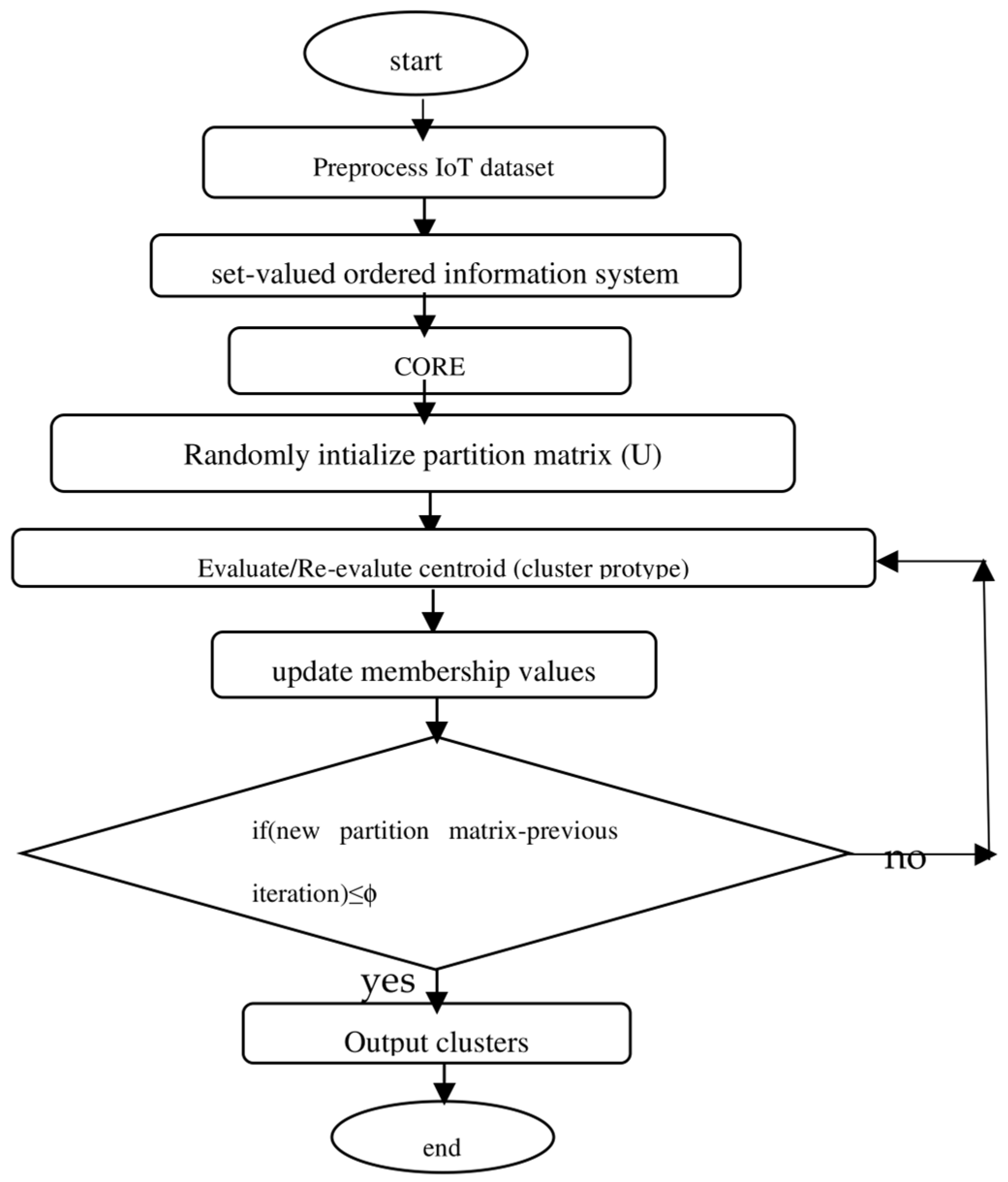
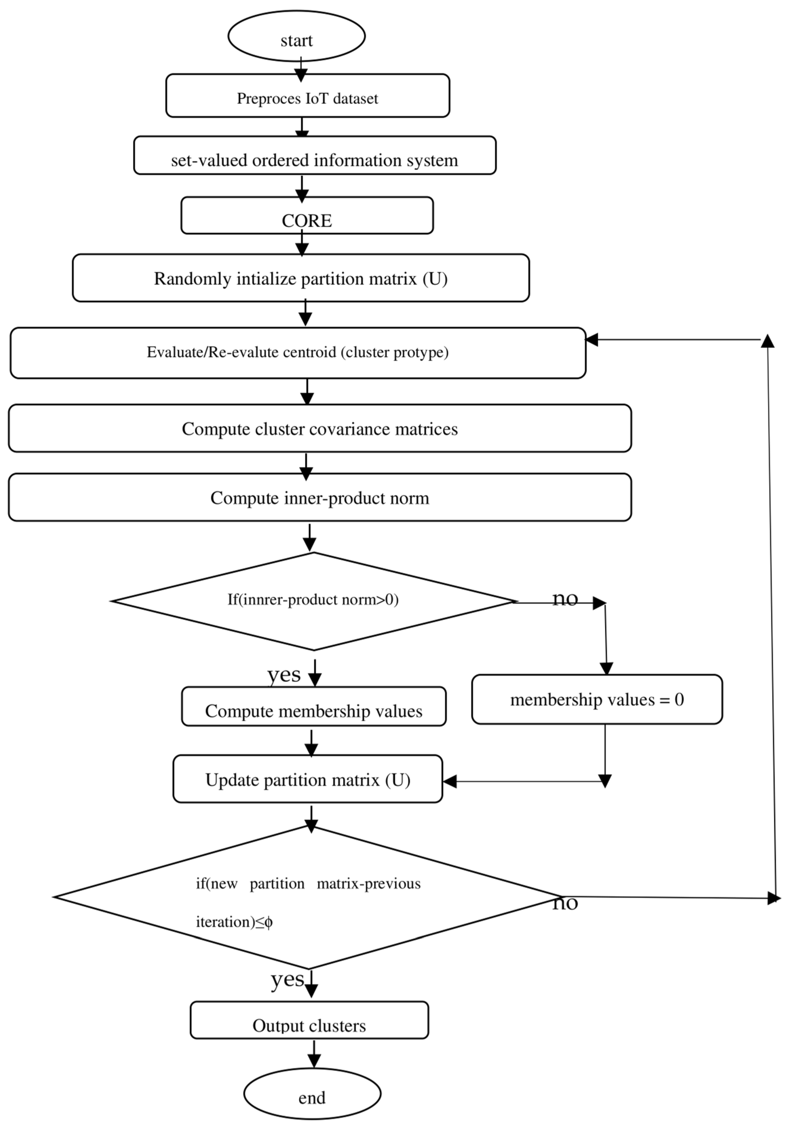
3. Proposed Methods

The methods proposed in this article are a two-staged hybrid approach consisting of subspace generation and fuzzy clustering algorithms. In stage 1, the rough set-based approach is used to generate subspace. In stage 2, fuzzy clustering methods are employed to generate fuzzy clusters. The stage 1 of the proposed method is described as follows. Our dataset S = (U, A) is an information system consisting of both conditional and decision attributes. First of all, a data pre-processing techniques is applied to convert it to set-valued ordered information system. Then, a dominance relation, a nano topology and its basis, is generated. Then, the criterion reduction process is used to generate CORE (A) as a subset of A. This way new information system E = (U, CORE (A)) ⊆ S is computed. The pseudocode of the algorithm for the criterion reduction is given below (Algorithm 1).

Algorithm 1: Nano Topology-based Subspace Generation

Input. (U, A): the information system, where the attribute set A is divided into C-conditional attributes and D-decision attributes, consisting of n data instances. Output: Subspace of (U, A) Step 1. Generate a dominance relation $R_C^{\ge }$ on U corresponding to C and X ⊆ U. Step 2. Generate the Nano topology ${\tau }_C^{\ge }\left(X\right)$ and its basis ${\beta }_C^{\ge }\left(X\right)$ Step 3. for each x ∈ C, find ${\tau }_{C-\left\{x\right\}}^{\ge }\left(X\right)$ and ${\beta }_{C-\left\{x\right\}}^{\ge }\left(X\right)$ Step 4.   if (${\beta }_C^{\ge }\left(X\right)={\beta }_{C-\left\{x\right\}}^{\ge }\left(X\right)$) Step 5.       then drop x from C, Step 6.   else form criterion reduction Step 7.     end for Step 8. generate CORE(C) = ∩{criterion reductions} Step 9. Generate subspace of the given information system.

The above algorithm supplies the CORE of the attribute set by removing insignificant attributes which gives us a subspace E = (U, CORE (A)) of the given information system S = (U, A). Since, the nano topology is generated for the generation of CORE. The above algorithm is named the nano topology-based subspace generation algorithm. Then, stage 2 of the method starts. For stage 2, different variations of fuzzy clustering algorithms are explored. The algorithms are described as follows.

3.1. Fuzzy C-Means (FCM) Algorithm [41]

A large class of the FCM algorithms is based on the minimization of fuzzy c-means functional formulated as follows.

$$\mathit{J}\left(\mathit{X};\mathit{U},\mathit{V}\right)={\sum }_{\mathit{i}=}^{\mathit{c}}{\sum }_{\mathit{k}=\mathbf{1}}^{\mathit{N}}({\mathit{\mu }}_{\mathit{i}\mathit{k}}{)}^{\mathit{m}}{‖{\mathit{x}}_{\mathit{k}}-{\mathit{v}}_{\mathit{i}}‖}_{\mathit{A}}^{\mathbf{2}}$$

(9)

where U = [μ_ik] ∈ F_fc (fuzzy partition of X) and V = [v₁, v₂,…, v_c], v_i ∈ Rⁿ, a vector of cluster’s mean, which need to be computed.

${\mathit{D}}_{\mathit{i}\mathit{k}\mathit{A}}^{\mathbf{2}}={‖{\mathit{x}}_{\mathit{k}}-{\mathit{v}}_{\mathit{i}}‖}_{\mathit{A}}^{\mathbf{2}}={\left({\mathit{x}}_{\mathit{k}}-{\mathit{v}}_{\mathit{i}}\right)}^{\mathit{T}}\mathit{A}({\mathit{x}}_{\mathit{k}}-{\mathit{v}}_{\mathit{i}})$ is the squared inner-product norm, and m ∈ [1, ∝] decides the resulting cluster’s fuzziness. Equation (9) measures the total variance of x_k from v_i.

The minimization of (9) is a non-linear optimization problem and can be solved by various methods like Picard’s iteration method. The first-order conditions of stationary points through Picard’s iteration method is known as the fuzzy c-means algorithm (FCM) (Algorithm 2) [41].

The stationary points of (9) can be obtained by adjoining constraints to J with Lagrange’s multipliers [41].

$$\mathit{J}\left(\mathit{X};\mathit{U},\mathit{V},\mathit{\lambda }\right)={\sum }_{\mathit{i}=}^{\mathit{c}}{\sum }_{\mathit{k}=\mathbf{1}}^{\mathit{N}}({\mathit{\mu }}_{\mathit{i}\mathit{k}}{)}^{\mathit{m}}{\mathit{D}}_{\mathit{i}\mathit{k}\mathit{A}}^{\mathbf{2}}+{\sum }_{\mathit{k}=}^{\mathit{N}}{\mathit{\lambda }}_{\mathit{k}}\left[{\sum }_{\mathit{i}=\mathbf{1}}^{\mathit{c}}{\mathit{\mu }}_{\mathit{i}\mathit{k}}-\mathbf{1}\right]$$

(10)

By setting the partial derivatives of J with respect to U, V and λ are 0, if ${\mathit{D}}_{\mathit{i}\mathit{k}\mathit{A}}^{\mathbf{2}}>\mathbf{0}$ ∀ i, k and m > 1, then (U, V) ∈ F_fc × R^c×n will minimize only if

$${\mathit{\mu }}_{\mathit{i}\mathit{k}}=\frac{\mathbf{1}}{{\left({\mathit{D}}_{\mathit{i}\mathit{k}\mathit{A}/{\mathit{D}}_{\mathit{j}\mathit{k}\mathit{A}}}\right)}^{\mathbf{2}/(\mathit{m}-\mathbf{1})}}, 1\le i\le c, 1\le k\le N$$

(11)

and

$${\mathit{v}}_{\mathit{i}}=\frac{\sum _{\mathit{k}=\mathbf{1}}^{\mathit{N}}({\mathit{\mu }}_{\mathit{i}\mathit{k}}{)}^{\mathit{m}}{\mathit{x}}_{\mathit{k}}}{\sum _{\mathit{k}=\mathbf{1}}^{\mathit{N}}({\mathit{\mu }}_{\mathit{i}\mathit{k}}{)}^{\mathit{m}}}, 1\le i\le c$$

(12)

The above solutions, (11) and (12), also satisfy (8) and are the first-order necessary conditions for the existence of stationary points of the objective function (9).

Algorithm 2: (FCM)

Given dataset X, choose the number of cluster c, (1 < c < N), weighting exponent m > 1, terminating threshold ϕ > 0, and A (norm-inducing matrix). Initialize U = U(0) // U(0) ∈ Ffc for each j = 1, 2,…… step 1 compute cluster mean ${\mathit{v}}_{\mathit{i}}^{\left(\mathit{j}\right)}=\frac{\sum _{\mathit{k}=\mathbf{1}}^{\mathit{N}}{\left({\mathit{\mu }}_{\mathit{i}\mathit{k}}^{(\mathit{j}-\mathbf{1})}\right)}^{\mathit{m}}{\mathit{x}}_{\mathit{k}}}{\sum _{\mathit{k}=\mathbf{1}}^{\mathit{N}}{\left({\mathit{\mu }}_{\mathit{i}\mathit{k}}^{(\mathit{j}-\mathbf{1})}\right)}^{\mathit{m}}}$, i = 1, 2,…, c step 2 compute  ${\mathit{D}}_{\mathit{i}\mathit{k}\mathit{A}}^{\mathbf{2}}={\left({\mathit{x}}_{\mathit{k}}-{\mathit{v}}_{\mathit{i}}^{\left(\mathit{j}\right)}\right)}^{\mathit{T}}\mathit{A}({\mathit{x}}_{\mathit{k}}-{\mathit{v}}_{\mathit{i}}^{\left(\mathit{j}\right)})$, i = 1, 2,…, c, k = 1, 2,…, N step 3 for k = 1, 2,…, N // update partition matrix if DikA > 0, for all i = 1, 2,…, c ${\mathit{\mu }}_{\mathit{i}\mathit{k}}^{\left(\mathit{j}\right)}=\frac{\mathbf{1}}{\sum _{\mathit{l}=\mathbf{1}}^{\mathit{c}}{\left(\frac{{\mathit{D}}_{\mathit{i}\mathit{k}\mathit{A}}}{{\mathit{D}}_{\mathit{l}\mathit{k}\mathit{A}}}\right)}^{\mathbf{2}/(\mathit{m}-\mathbf{1})}}$, else ${\mathit{\mu }}_{\mathit{i}\mathit{k}}^{\left(\mathit{j}\right)}$ = 0 if DikA > 0, ${\mathit{\mu }}_{\mathit{i}\mathit{k}}^{\left(\mathit{j}\right)}\mathit{ϵ}[\mathbf{0}\mathbf{,}\mathbf{1}]$ with $\sum _{\mathit{i}=\mathbf{1}}^{\mathit{c}}{\mathit{\mu }}_{\mathit{i}\mathit{k}}^{\left(\mathit{j}\right)}$ = 1 until ||U(j)-U(j−1)|| < ϕ

3.2. Definition 2.11 [48]

Euclidean distance, though used many times in clustering-based anomaly detection algorithms, has limitations. Euclidean distance measures the shortest distance between two points. Euclidean distance does not take into consideration the correlation between the attribute values, so Euclidean distance assigns equal weight to such variables which essentially measure the same feature. Therefore, this single feature gains extra weight. Consequently, correlated variables gain excess weight by Euclidean distance which affects accuracy. Since the IoT data are highly correlated, it is preferable to use Mahalanobis distance instead, as it takes into account the correlation between the variables. It is a scale-invariant metric which gives distance between a point x ∈ Rⁿ generated from a given p-variant probability distribution P_X (.) and the distribution’s mean μ = E (X). Suppose P_X (.) has finite second-order moments and ∑ = E (X – μ), the covariance matrix, then the Mahalanobis distance [43,44,47] is given by

$$d(X,\mu )=\sqrt{(X-\mu ){\sum }^{-1}(X-\mu )}$$

(13)

If the covariance matrix is an identity matrix, the Mahalanobis distance reduces to the Euclidean distance.

3.3. Gustafson–Kessel (GK) Algorithm [42,47]

This is an extension of FCM where an adaptive distance norm was used to detect clusters of various shapes from one dataset. Each cluster has its own norm-inducing matrix A_i, which produces the inner-product norm given below.

$${\mathit{D}}_{\mathit{i}\mathit{k}{\mathit{A}}_{\mathit{i}}}^{\mathbf{2}}={\left({\mathit{x}}_{\mathit{k}}-{\mathit{v}}_{\mathit{i}}\right)}^{\mathit{T}}{\mathit{A}}_{\mathit{i}}({\mathit{x}}_{\mathit{k}}-{\mathit{v}}_{\mathit{i}})$$

(14)

The matrices A_i are used as optimization variables in the c-means functional, which allows for each cluster to adapt the distance norm to the local topological structure of the data. The objective function of the GK algorithm is given by

$$\mathit{J}\left(\mathit{X};\mathit{U},\mathit{V},{\{\mathit{A}}_{\mathit{i}}\}\right)={\sum }_{\mathit{i}=\mathbf{1}}^{\mathit{c}}{\sum }_{\mathit{k}=\mathbf{1}}^{\mathit{N}}({\mathit{\mu }}_{\mathit{i}\mathit{k}}{)}^{\mathit{m}}{\mathit{D}}_{{\mathit{i}\mathit{k}\mathit{A}}_{\mathit{i}}}^{\mathbf{2}}$$

(15)

where A_i = |Σ_i|^1/p Σ_i⁻¹

$${\sum }_{\mathit{i}}={\left|{\sum }_{\mathit{i}=\mathbf{1}}^{\mathit{c}}{\sum }_{\mathit{k}=\mathbf{1}}^{\mathit{N}}({\mathit{\mu }}_{\mathit{i}\mathit{k}}{)}^{\mathit{m}}\right|}^{-\mathbf{1}}{\sum }_{\mathit{i}=\mathbf{1}}^{\mathit{c}}{\sum }_{\mathit{k}=\mathbf{1}}^{\mathit{N}}{\mathit{\mu }}_{\mathit{i}\mathit{k}}({\mathit{x}}_{\mathit{k}}-{\mathit{v}}_{\mathit{i}})({\mathit{x}}_{\mathit{k}}-{\mathit{v}}_{\mathit{i}}{)}^{\mathit{T}}$$

(16)

The GK algorithm (Algorithm 3) for fuzzy clustering is given below.

Algorithm 3: (GK)

Given dataset X, choose the number of cluster c, (1 < c < N), weighting exponent m > 1, terminating threshold ϕ > 0, and cluster volume M. Initialize U = U(0) // U(0) ∈ Ffc for each j = 1, 2,…… step 1 compute cluster mean ${\mathit{v}}_{\mathit{i}}^{\left(\mathit{j}\right)}=\frac{\sum _{\mathit{k}=\mathbf{1}}^{\mathit{N}}{\left({\mathit{\mu }}_{\mathit{i}\mathit{k}}^{(\mathit{j}-\mathbf{1})}\right)}^{\mathit{m}}{\mathit{x}}_{\mathit{k}}}{\sum _{\mathit{k}=\mathbf{1}}^{\mathit{N}}{\left({\mathit{\mu }}_{\mathit{i}\mathit{k}}^{(\mathit{j}-\mathbf{1})}\right)}^{\mathit{m}}}$, i = 1, 2,…c step 2 compute the cluster covariance matrices ${\mathit{C}}_{\mathit{i}}=\frac{\sum _{\mathit{k}=\mathbf{1}}^{\mathit{N}}{\left({\mathit{\mu }}_{\mathit{i}\mathit{k}}^{(\mathit{j}-\mathbf{1})}\right)}^{\mathit{m}}\left({\mathit{x}}_{\mathit{k}}-{\mathit{v}}_{\mathit{i}}^{\mathit{j}}\right){\left({\mathit{x}}_{\mathit{k}}-{\mathit{v}}_{\mathit{i}}^{\mathit{j}}\right)}^{\mathit{T}}}{\sum _{\mathit{k}=\mathbf{1}}^{\mathit{N}}{\left({\mathit{\mu }}_{\mathit{i}\mathit{k}}^{(\mathit{j}-\mathbf{1})}\right)}^{\mathit{m}}}$, i = 1, 2,…, c step 3 compute ${\mathit{D}}_{\mathit{i}\mathit{k}{\mathit{A}}_{\mathit{i}}}^{\mathbf{2}}$ (for i = 1, 2,…, c, k = 1, 2,…, N) using Equations (14) and (16) step 4 for k = 1, 2,…, N // update partition matrix if DikA > 0, for all i = 1, 2,…, c ${\mathit{\mu }}_{\mathit{i}\mathit{k}}^{\left(\mathit{j}\right)}=\frac{\mathbf{1}}{\sum _{\mathit{l}=\mathbf{1}}^{\mathit{c}}{\left(\frac{{\mathit{D}}_{\mathit{i}\mathit{k}\mathit{A}}}{{\mathit{D}}_{\mathit{l}\mathit{k}\mathit{A}}}\right)}^{\mathbf{2}/(\mathit{m}-\mathbf{1})}}$, else ${\mathit{\mu }}_{\mathit{i}\mathit{k}}^{\left(\mathit{j}\right)}$ = 0 if DikA > 0, ${\mathit{\mu }}_{\mathit{i}\mathit{k}}^{\left(\mathit{j}\right)}\mathit{ϵ}[\mathbf{0},\mathbf{1}]$ with $\sum _{\mathit{i}=\mathbf{1}}^{\mathit{c}}{\mathit{\mu }}_{\mathit{i}\mathit{k}}^{\left(\mathit{j}\right)}$ = 1 until ||U(j)-U(j−1)|| < ϕ

3.4. Gath–Geva Algorithm (GG) [43,47]

Gath and Geva [43,47] proposed an extension of the GK algorithm by introducing maximum likelihood estimates instead of Euclidean distance which can be used to detect clusters of varying shapes, sizes, and densities. The objective function of the algorithm is given by

$$\mathit{J}\left(\mathit{X};\mathit{U},\mathit{V},{\{\mathit{A}}_{\mathit{i}}\}\right)={\sum }_{\mathit{i}=\mathbf{1}}^{\mathit{c}}{\sum }_{\mathit{k}=\mathbf{1}}^{\mathit{N}}({\mathit{\mu }}_{\mathit{i}\mathit{k}}{)}^{\mathit{m}}{\mathit{D}}_{{\mathit{i}\mathit{k}\mathit{A}}_{\mathit{i}}}^{\mathbf{2}}$$

(17)

where ${\mathit{D}}_{{\mathit{i}\mathit{k}\mathit{A}}_{\mathit{i}}}^{\mathbf{2}}$ is the Gauss distance between x_k and the cluster mean v_i and is given by

$${\mathit{D}}_{{\mathit{i}\mathit{k}\mathit{A}}_{\mathit{i}}}^{\mathbf{2}}=\frac{(\mathbf{2}\mathit{\pi }{)}^{\mathit{N}/\mathbf{2}}\sqrt{\left|{\mathit{A}}_{\mathit{i}}\right|}}{{\mathit{\alpha }}_{\mathit{i}}}\mathbf{e}\mathbf{x}\mathbf{p}\left(\frac{\mathbf{1}}{\mathbf{2}}{\left({\mathit{x}}_{\mathit{k}}-{\mathit{v}}_{\mathit{i}}\right)}^{\mathit{T}}{\mathit{A}}_{\mathit{i}}^{-\mathbf{1}}\left({\mathit{x}}_{\mathit{k}}-{\mathit{v}}_{\mathit{i}}\right)\right)$$

(18)

and

$${\mathit{A}}_{\mathit{i}}=\frac{\sum _{\mathit{k}=\mathbf{1}}^{\mathit{N}}{\left({\mathit{\mu }}_{\mathit{i}\mathit{k}}\right)}^{\mathit{m}}\left({\mathit{x}}_{\mathit{k}}-{\mathit{v}}_{\mathit{i}}\right){\left({\mathit{x}}_{\mathit{k}}-{\mathit{v}}_{\mathit{i}}\right)}^{\mathit{T}}}{\sum _{\mathit{k}=\mathbf{1}}^{\mathit{N}}{\left({\mathit{\mu }}_{\mathit{i}\mathit{k}}\right)}^{\mathit{m}}}, i = 1, 2,\dots ,c$$

(19)

Also, α_i is the a priori probability of x_k belonging to the ith cluster and is given by

$${\mathit{\alpha }}_{\mathit{i}}=\frac{\sum _{\mathit{k}=\mathbf{1}}^{\mathit{N}}{\left({\mathit{\mu }}_{\mathit{i}\mathit{k}}\right)}^{\mathit{m}}}{\mathit{N}}$$

(20)

The objective function (17) is minimized by the following equations:

$${\mathit{\mu }}_{\mathit{i}\mathit{k}}=\frac{\mathbf{1}}{\sum _{\mathit{l}=\mathbf{1}}^{\mathit{c}}{\left(\frac{{\mathit{D}}_{\mathit{i}\mathit{k}{\mathit{A}}_{\mathit{i}}}}{{\mathit{D}}_{\mathit{j}\mathit{k}\mathit{A}\mathit{j}}}\right)}^{\mathbf{1}/(\mathit{m}-\mathbf{1})}}, 1\le j\le c, 1\le k\le N$$

(21)

and

$${\mathit{v}}_{\mathit{i}}=\frac{\sum _{\mathit{k}=\mathbf{1}}^{\mathit{N}}{\left({\mathit{\mu }}_{\mathit{i}\mathit{k}}\right)}^{\mathit{m}}{\mathit{x}}_{\mathit{k}}}{\sum _{\mathit{k}=\mathbf{1}}^{\mathit{N}}{\left({\mathit{\mu }}_{\mathit{i}\mathit{k}}\right)}^{\mathit{m}}}$$

(22)

As the algorithm uses the exponential distance norm, it requires a good initialization (Algorithm 4).

Algorithm 4: (GG)

Given dataset X, choose the number of cluster c, (1 < c < N), and terminating threshold ϕ > 0. Initialize U = U(0) // U(0) ∈ Ffc step 1 compute cluster mean vi step 2 calculate the distance measure using Equation (18) step 3 calculate Ai step 3 calculate the value of the membership data function using equation (21) and update U, the partition matrix until ||U(j)-U(j−1)|| < ϕ

3.5. Mahalanobis Distance-Based Fuzzy C-Means algorithm (M-FCM) [47]

The objective function of the M-FCM algorithm is given by

$$\mathit{J}\left(\mathit{X};\mathit{U},\mathit{V},\mathit{\sum }\right)={\sum }_{\mathit{i}=}^{\mathit{c}}{\sum }_{\mathit{k}=\mathbf{1}}^{\mathit{N}}({\mathit{\mu }}_{\mathit{i}\mathit{k}}{)}^{\mathit{m}}{\mathit{D}}_{\mathit{i}\mathit{k}}^{\mathbf{2}}$$

(23)

such that

$$m\in [\mathbf{1}, \propto ], U=[{\mathsf{\mu }}_{\mathrm{ik}}{]}_{c\times n}, {\mathsf{\mu }}_{\mathrm{ik}}\in [0, 1], i=1, 2,\dots , c; k=1, 2,\dots , n, {\sum }_{\mathit{i}=\mathbf{1}}^{\mathit{c}}{\mathit{\mu }}_{\mathit{i}\mathit{k}}=\mathbf{1}, k=1, 2,\dots , n, \mathbf{0}<{\sum }_{\mathit{k}=\mathbf{1}}^{\mathit{n}}{\mathit{\mu }}_{\mathit{i}\mathit{k}}<\mathit{N}, i = 1, 2, \dots ,c$$

(24)

$${\mathit{D}}_{\mathit{i}\mathit{k}}^{\mathbf{2}}=\left\{\begin{array}{c}({\mathit{x}}_{\mathit{k}}-{\mathit{v}}_{\mathit{i}}{)}^{\mathit{T}}{\sum }_{\mathit{i}}^{-\mathbf{1}}\left({\mathit{x}}_{\mathit{k}}-{\mathit{v}}_{\mathit{i}}\right)-\mathit{l}\mathit{n}\left|{\sum }_{\mathit{i}}^{-\mathbf{1}}\right|,\mathit{i}\mathit{f}({\mathit{x}}_{\mathit{k}}-{\mathit{v}}_{\mathit{i}}{)}^{\mathit{T}}{\sum }_{\mathit{i}}^{-\mathbf{1}}\left({\mathit{x}}_{\mathit{k}}-{\mathit{v}}_{\mathit{i}}\right)-\mathit{l}\mathit{n}\left|{\sum }_{\mathit{i}}^{-\mathbf{1}}\right|\ge \mathbf{0}\\ \mathbf{0} \mathit{i}\mathit{f}({\mathit{x}}_{\mathit{k}}-{\mathit{v}}_{\mathit{i}}{)}^{\mathit{T}}{\sum }_{\mathit{i}}^{-\mathbf{1}}\left({\mathit{x}}_{\mathit{k}}-{\mathit{v}}_{\mathit{i}}\right)-\mathit{l}\mathit{n}\left|{\sum }_{\mathit{i}}^{-\mathbf{1}}\right|<\mathbf{0}\end{array}\right\}$$

(25)

Minimizing (23) with respect to all of its parameters subject to the constraints of (24) and (25) yields the M-FCM algorithm (Algorithm 5).

Algorithm 5: (M-FCM)

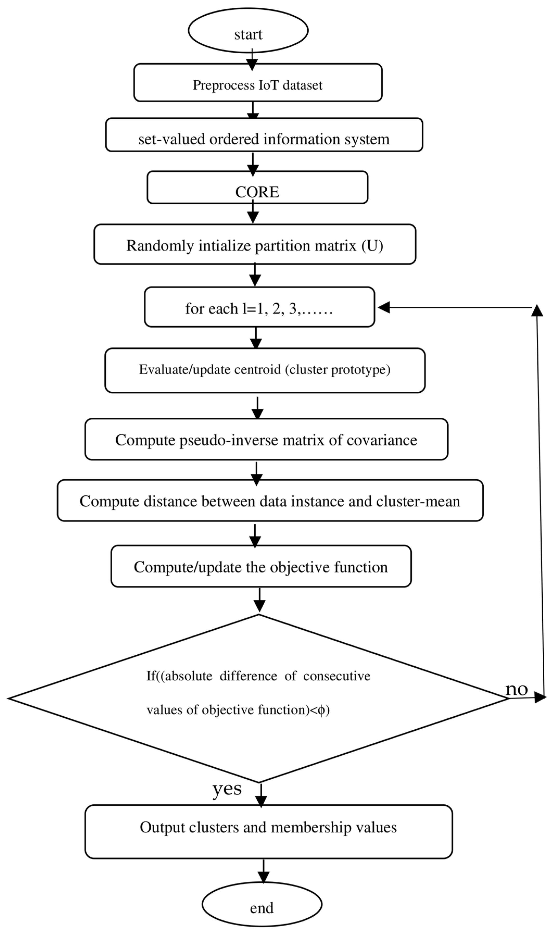
Given dataset X, choose the number of cluster c, (2 < c < N), weighting exponent m ∈ [0, ∝), iteration stop threshold ϕ > 0. Initialize randomly partition matrix (membership matrix) U subject to the constraint (24), iteration counter l = 1. step 1 Evaluate or update cluster-centroid vi; i = 1, 2,…, c. step 2 Evaluate pseudo-inverse matrix of covariance ${\sum }_{\mathit{i}}^{-\mathbf{1}}$ Step 3 Evaluate ${\mathit{D}}_{\mathit{i}\mathit{k}\mathit{\sum }\prime }^{\mathbf{2}}$ using (25) Step 4 Evaluate the value of the objective function (J) using (23) Step 5 Set l = l + 1 to update objective function J Step 6 If the value of the objective function obtained in step 3 satisfies $‖{\mathit{J}}^{\mathit{l}}-{\mathit{J}}^{\mathit{l}-\mathbf{1}}‖<\mathit{\varnothing }$, stop Output cluster set and membership matrix Step 7   Else go to step 1

3.6. Common Mahalanobis Distance-Based Fuzzy C-Means algorithm (CM-FCM) [47]

In this algorithm, all of the covariance matrices (${\sum }_{\mathit{i}})$ of the objective function are replaced with a common covariance matrix ($\sum$). The objective function of CM-FCM is given as follows:

$$\mathit{J}\left(\mathit{X};\mathit{U},\mathit{V},\mathit{\sum }\right)={\sum }_{\mathit{i}=}^{\mathit{c}}{\sum }_{\mathit{k}=\mathbf{1}}^{\mathit{N}}({\mathit{\mu }}_{\mathit{i}\mathit{k}}{)}^{\mathit{m}}{\mathit{D}}_{\mathit{i}\mathit{k}}^{\mathbf{2}}$$

(26)

subject to the constraints

$$m\in [1, \propto ], U=[{\mathsf{\mu }}_{\mathrm{ik}}{]}_{c\times n}, {\mathsf{\mu }}_{\mathrm{ik}}\in [0, 1], i=1, 2,\dots , c; k=1, 2,\dots , n, {\sum }_{\mathit{i}=\mathbf{1}}^{\mathit{c}}{\mathit{\mu }}_{\mathit{i}\mathit{k}}=\mathbf{1}, k=1, 2,\dots , n, \mathbf{0}<{\sum }_{\mathit{k}=\mathbf{1}}^{\mathit{n}}{\mathit{\mu }}_{\mathit{i}\mathit{k}}<\mathit{N}, i = 1, 2, \dots ,c$$

(27)

$${\mathit{D}}_{\mathit{i}\mathit{k}}^{\mathbf{2}}=\left\{\begin{array}{c}({\mathit{x}}_{\mathit{k}}-{\mathit{v}}_{\mathit{i}}{)}^{\mathit{T}}{\sum }^{-\mathbf{1}}\left({\mathit{x}}_{\mathit{k}}-{\mathit{v}}_{\mathit{i}}\right)-\mathit{l}\mathit{n}\left|{\sum }^{-\mathbf{1}}\right|,\mathit{i}\mathit{f}({\mathit{x}}_{\mathit{k}}-{\mathit{v}}_{\mathit{i}}{)}^{\mathit{T}}{\sum }^{-\mathbf{1}}\left({\mathit{x}}_{\mathit{k}}-{\mathit{v}}_{\mathit{i}}\right)-\mathit{l}\mathit{n}\left|{\sum }^{-\mathbf{1}}\right|\ge \mathbf{0}\\ \mathbf{0} \mathit{i}\mathit{f}({\mathit{x}}_{\mathit{k}}-{\mathit{v}}_{\mathit{i}}{)}^{\mathit{T}}{\sum }^{-\mathbf{1}}\left({\mathit{x}}_{\mathit{k}}-{\mathit{v}}_{\mathit{i}}\right)-\mathit{l}\mathit{n}\left|{\sum }^{-\mathbf{1}}\right|<\mathbf{0}\end{array}\right\}$$

(28)

Minimizing the objective function (26) with respect to its parameters subject to the constraints (27) and (28) gives the CM-FCM algorithm (Algorithm 6).

Algorithm 6: (CM-FCM)

Given dataset X, choose the number of cluster c, (2 < c < N), weighting exponent m ∈ [0, ∝), iteration stop threshold ϕ > 0. Initialize randomly partition matrix (membership matrix) U subject to the constraint (27), iteration counter l = 1. step 1 Evaluate or update cluster-centroid vi; i = 1, 2,…, c. step 2 Evaluate pseudo-inverse matrix of covariance ${\sum }^{-\mathbf{1}}$ Step 3 Evaluate ${\mathit{D}}_{\mathit{i}\mathit{k}\mathit{\sum }\prime }^{\mathbf{2}}$ using (28) step 3 Evaluate the value of the objective function (J) using (26) step 4 Set l = l+1 to update objective function J Step 5 If the value of the objective function obtained in step 3 satisfies $‖{\mathit{J}}^{\mathit{l}}-{\mathit{J}}^{\mathit{l}-\mathbf{1}}‖<\mathit{\varnothing }$, stop Output cluster set and membership matrix Step 6 Else go to step 1

It is to be mentioned here that when the covariance matrices become identity matrices, CM-FCM becomes FCM. Thus, FCM is a special case of the CM-FCM algorithm.

Here, each cluster in the final output cluster set is a fuzzy set consisting of IoT data instances along with their membership grades. The IoT data instances which belong to all fuzzy clusters with minimum membership values would be treated as anomalies. A flowchart of the nano topology-based fuzzy c-means clustering algorithm is given in Figure 1 below.

The above Figure depicts a concise view of the NT-FCM clustering algorithm. It has the following main components. First of all, the method computes CORE, a lower dimensional space of the dataset by generating nano topology and basis. Then, the steps of FCM like initialization, membership assignment, cluster-center update, convergence check, iteration counter update, and finally stopping criteria check are executed. It illustrates the iterative process of adjusting cluster memberships and updating cluster centers until convergence is achieved in a lower dimensional space. This method supplies a set of fuzzy clusters in the lower dimensional space.

A flowchart of the nano topology-based GK clustering algorithm is given in Figure 2 below.

Figure 2 illustrates the iterative process of NT-GK clustering algorithm. It is an extension of the NT-FCM clustering algorithm where an adaptive distance norm was used to detect clusters of various shapes from one dataset. All other steps are similar to Figure 1. Each cluster has its own norm-inducing matrix. The method supplies a set of fuzzy clusters in the lower dimensional space.

A flowchart of the nano topology-based GG clustering algorithm is given in Figure 3 below.

Figure 3 illustrates the iterative process of the NT-GG clustering algorithm. It is an extension of the NT-GK algorithm which uses maximum likelihood estimates instead of Euclidean distance and is used to detect clusters of varying shapes, sizes, and densities. All other steps of the algorithm are similar to NT-FCM and NT-GK fuzzy clustering algorithms. As usual, the method supplies a set of fuzzy clusters in the lower dimensional space.

A flowchart of the Nano topology and Mahalanobis Distance-based Fuzzy C-Means algorithm (NT-M-FCM) is given in Figure 4 below.

Figure 4 represents the NT-M-FCM fuzzy clustering algorithm which uses Mahalanobis distance to enhance its performance, particularly in the scenarios where the data distribution is non-spherical or exhibits correlations among variables. It is useful in the situations where the assumption of equal variance in different dimensions may not hold. All other steps of the algorithm are similar to all the previous fuzzy clustering algorithms. Like all the previous methods, it also supplies a set of fuzzy clusters in the lower dimensional space.

A flowchart of the Nano topology and Common Mahalanobis Distance-based Fuzzy C-Means algorithm (NT-CM-FCM) is given in Figure 5 below.

The above Figure gives a concise view of the NT-CM-FCM clustering algorithm. It uses a common covariance matrix instead of different covariance matrices in the objective function. It is an extension of the NT-M-FCM clustering algorithm which incorporates a common Mahalanobis distance metric to account for the correlation between variables in the dataset. Like all the previous methods, it also supplies a set of fuzzy clusters in the lower dimensional space.

The approaches employed in this article consist of various combinations of the algorithms of the form (Algorithm 1 + Algorithm 2), (Algorithm 1 + Algorithm 3), (Algorithm 1 + Algorithm 4), (Algorithm 1 + Algorithm 5), and (Algorithm 1 + Algorithm 6), where Algorithm 1 (common to all) is used for dimension reduction and the others are used for clustering. The methods supply a specified number of fuzzy clusters in the lower dimensional space. The anomalous items are those IoT data instances which either do not belong or belong to clusters with minimum membership values.

4. Complexity Analysis

If |U| = m, and |C| = n, the worst-case time-complexity Algorithm 1 is O (m².n). Since FCM uses the norm-inducing matrix, the time complexity of the distance function of fuzzy clusters is O (c.(c − 1).d/2) = O (c².d). The worst-case complexity of FCM is O (m.c².d.i) = O (m.n.m².i) = O (m³.n.i), where d (≤n) is the dimension of the subspace generated by Algorithm 1, c (≤ m) is the number of fuzzy clusters, and I is the number of iterations. The overall time complexity of NT-FCM is O (m².n + m³.d.i). Obviously, i ≤ m and d ≤ n are small and can be neglected, and therefore, the overall worst-case time complexity of NT-FCM is O (m².n + m⁴), which shows that it is linear with respect to the dimension of the dataset. In general, n ≤ m, which gives the worst-case complexity as O (m⁴).

In finding the computational complexity of the NT-GK clustering algorithm, the complexity of NT is the same as O (m².n). For finding a new cluster and fuzzy c-means membership, the algorithm needs O I and O (n.c), which are same as FCM. In this algorithm, the most important task is that each cluster has its own norm-inducing matrix, which produces the inner product norm and the time complexity of such for c clusters is O (k (m.d.m.d)) = O (m².d²), where k is the constant time required for computing A_i. If i is the number of iterations, the overall time complexity is O (m².n + i. (c + n.c + c.m².d²)) = O (m².n + m².n + m⁴.d²) = O (m².n + m⁴.d²), where I = O (m), c = O (m), and d ≤ n ≤ m (in general) is small. Thus, the worst-case time complexity of the algorithm is O (m⁴.d²).

The GG fuzzy clustering algorithm uses the maximum likelihood estimation measure which requires O (m.d), as it uses the exponential distance which introduces another level of complexity. The time complexity of the NT-GG clustering algorithm is O (m².n + c. (m.c.d².i) = O (m².n + m⁴.d²), where I = O (m), c = O (m), and d ≤ n ≤ m (in general) is small. Thus, the worst-case time complexity of the algorithm is O (m⁴.d²).

The M-FCM computes separate matrices for each cluster, so the time complexity of the NT-M-FCM algorithm is O (m².n + i. (c + n.c + c.m.d²)) = O (m².n + m³.d²), where i = O (m), c = O (m), and d ≤ n ≤ m (in general) is small. Thus, the worst-case time complexity of the algorithm is O (m³.d²).

Since CM-FCM uses a common covariance matrix instead of separate covariance matrices of different clusters, the time complexity of the NT-CM-FCM algorithm is O (m².n + i. (c + n.c) + i.m.d²) = O (m².n + m².d²), where i = O (m), c = O (m), and d ≤ n ≤ m (in general) is small. Thus, the worst-case time complexity of the algorithm is O (m³ + m².d²).

5. Experimental Analysis, Results and Discussions

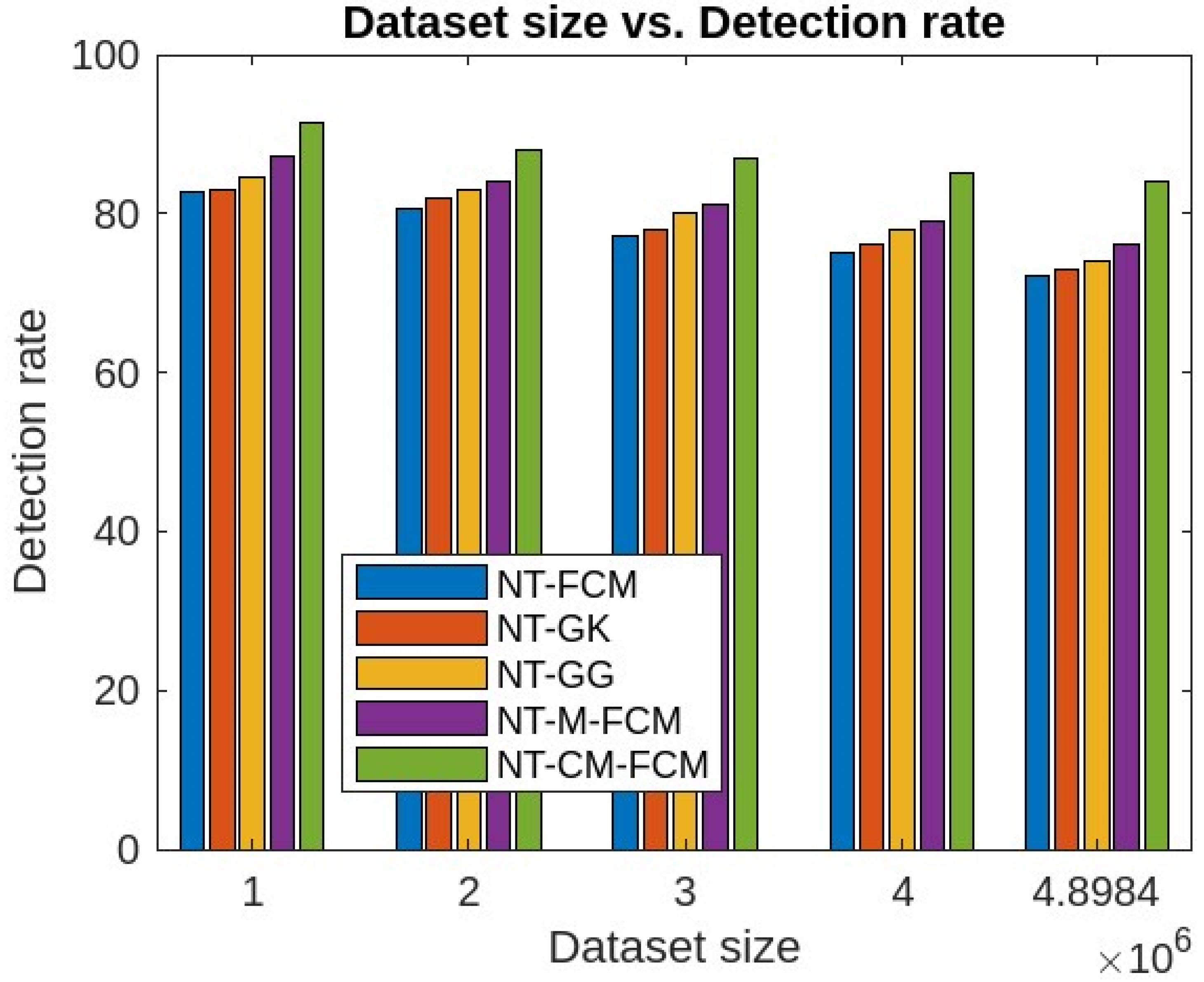
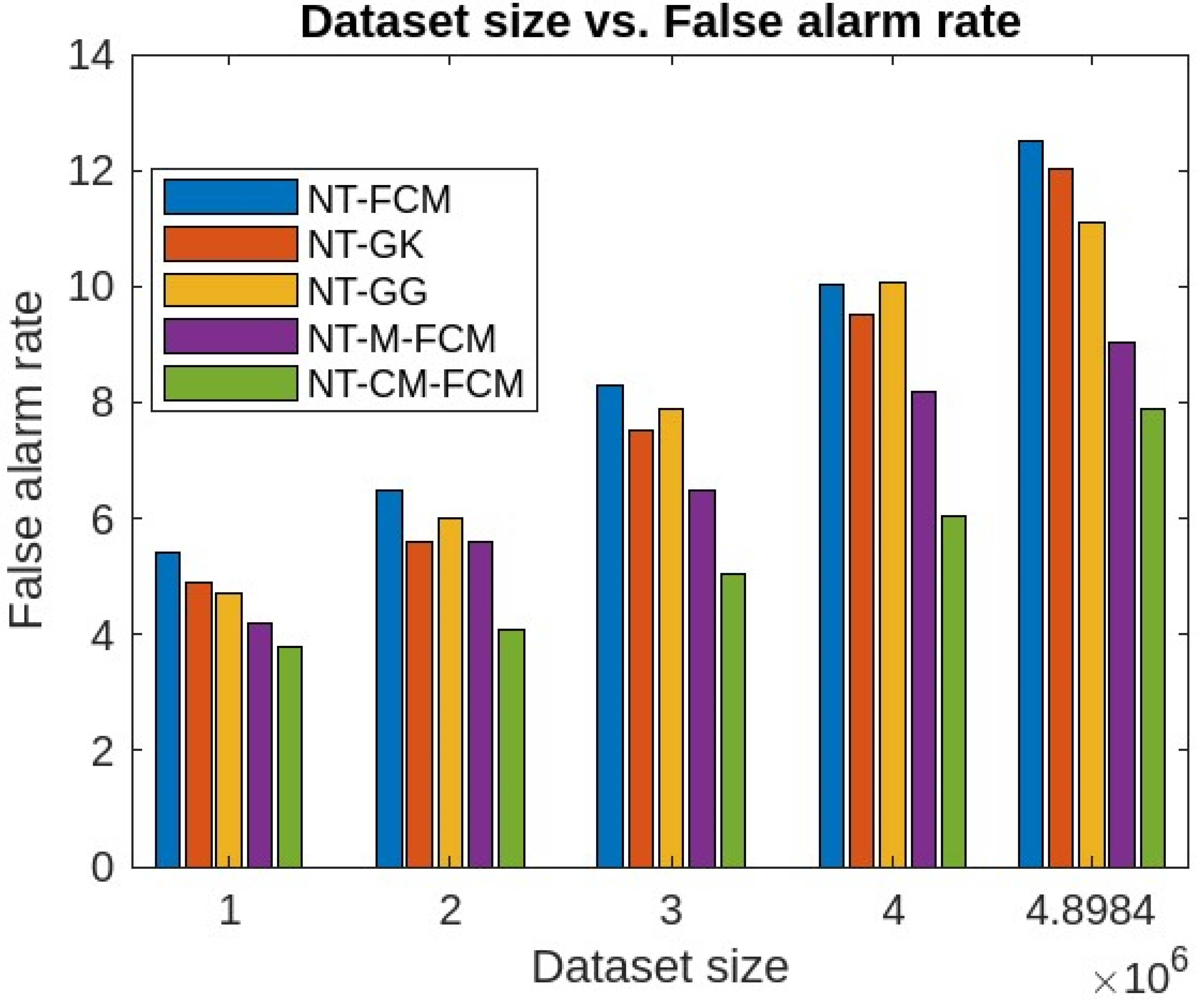
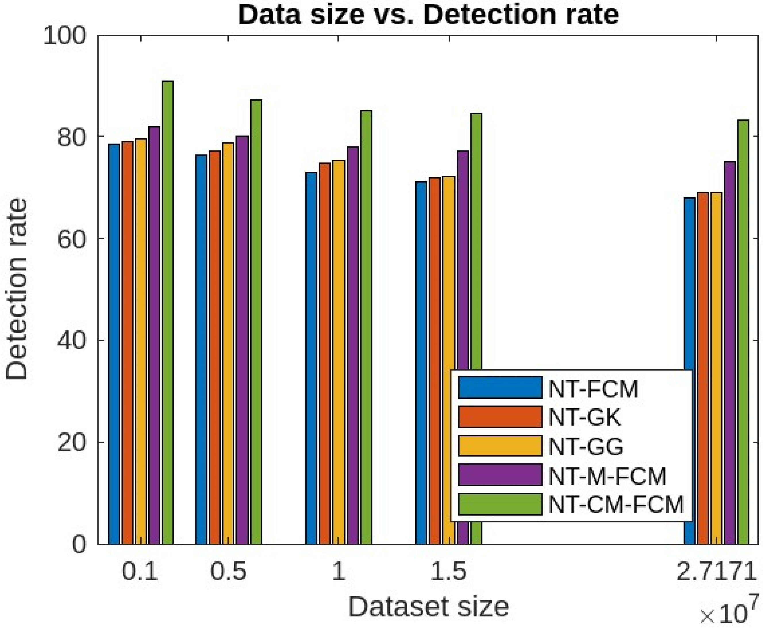
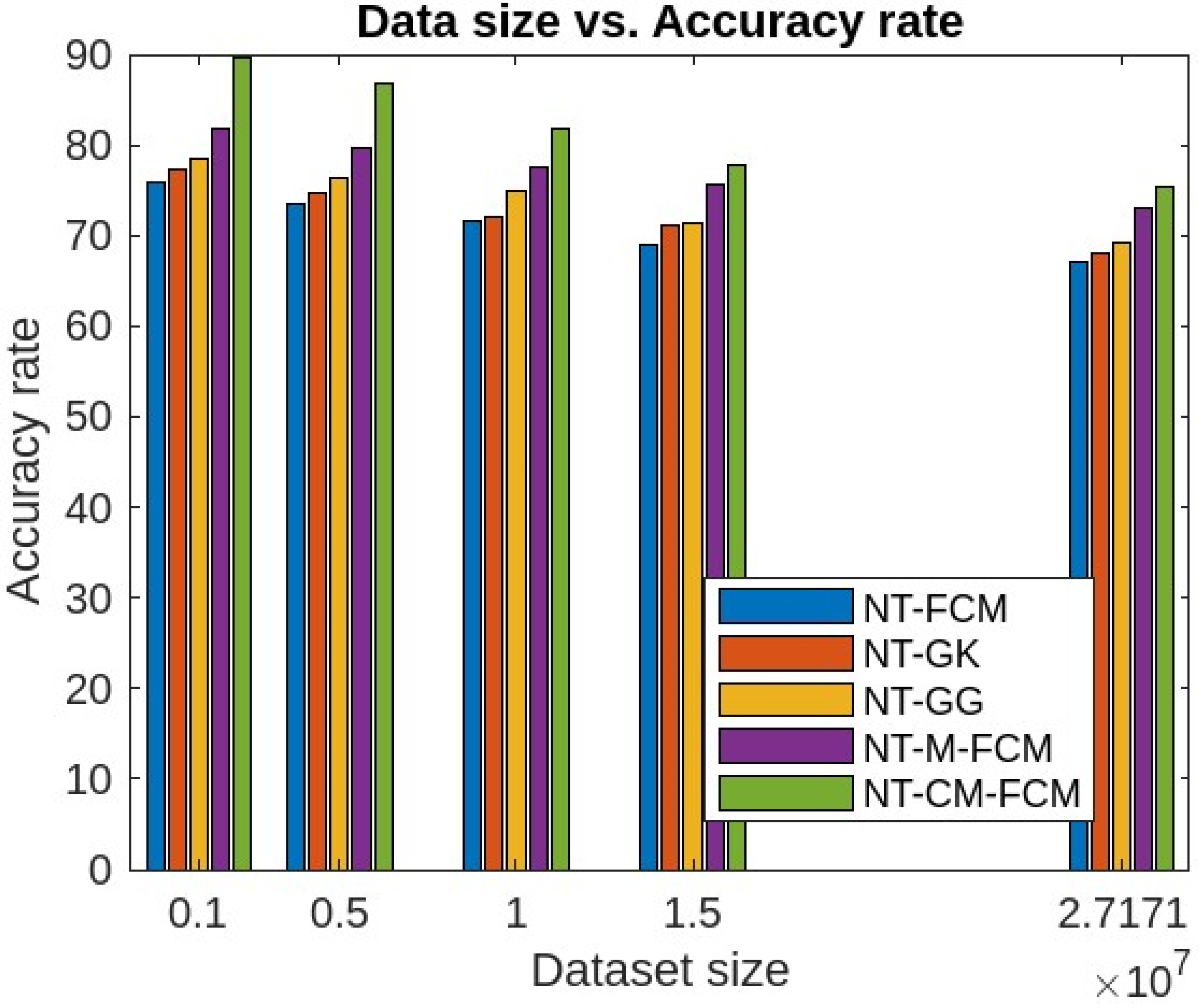
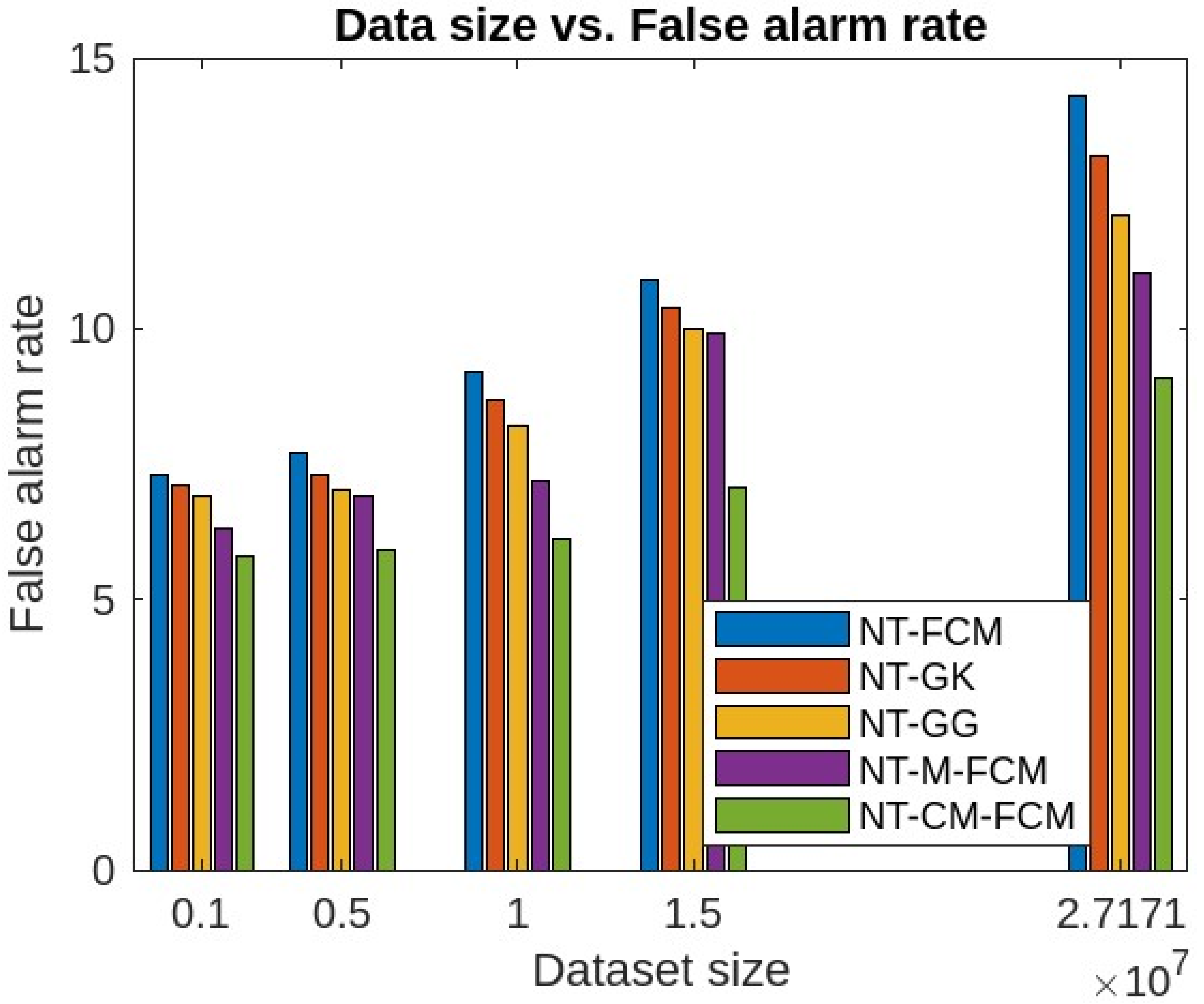
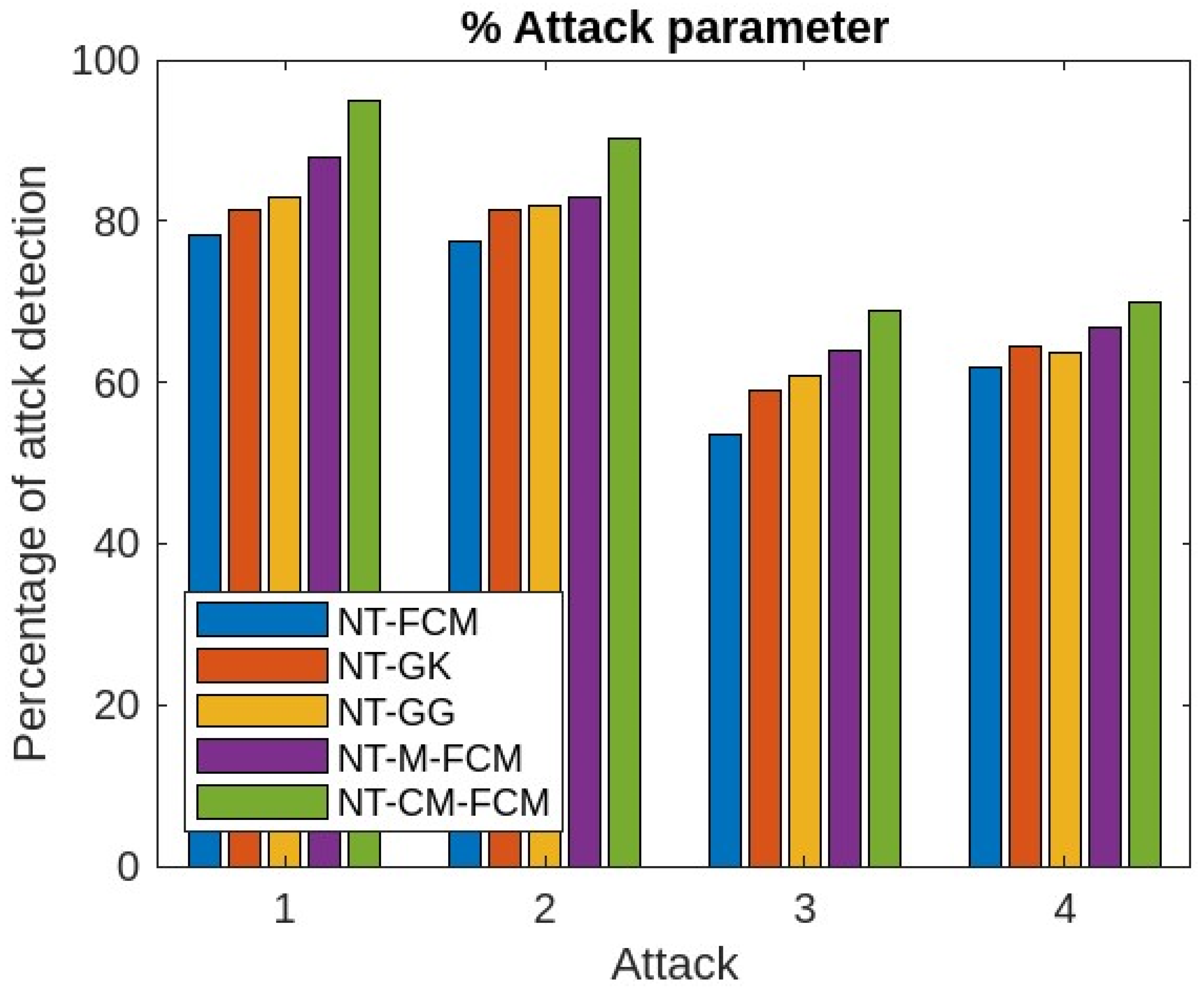
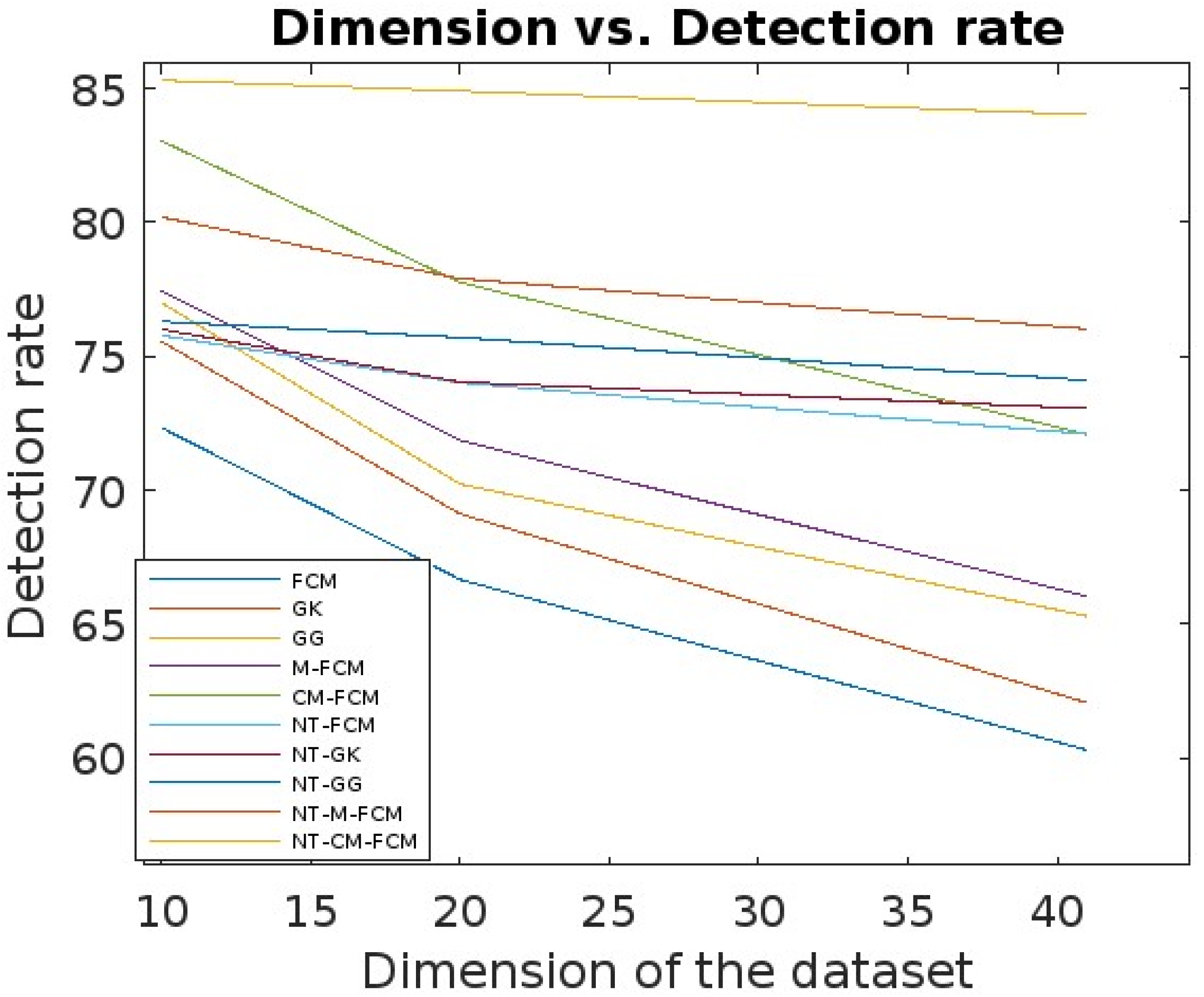
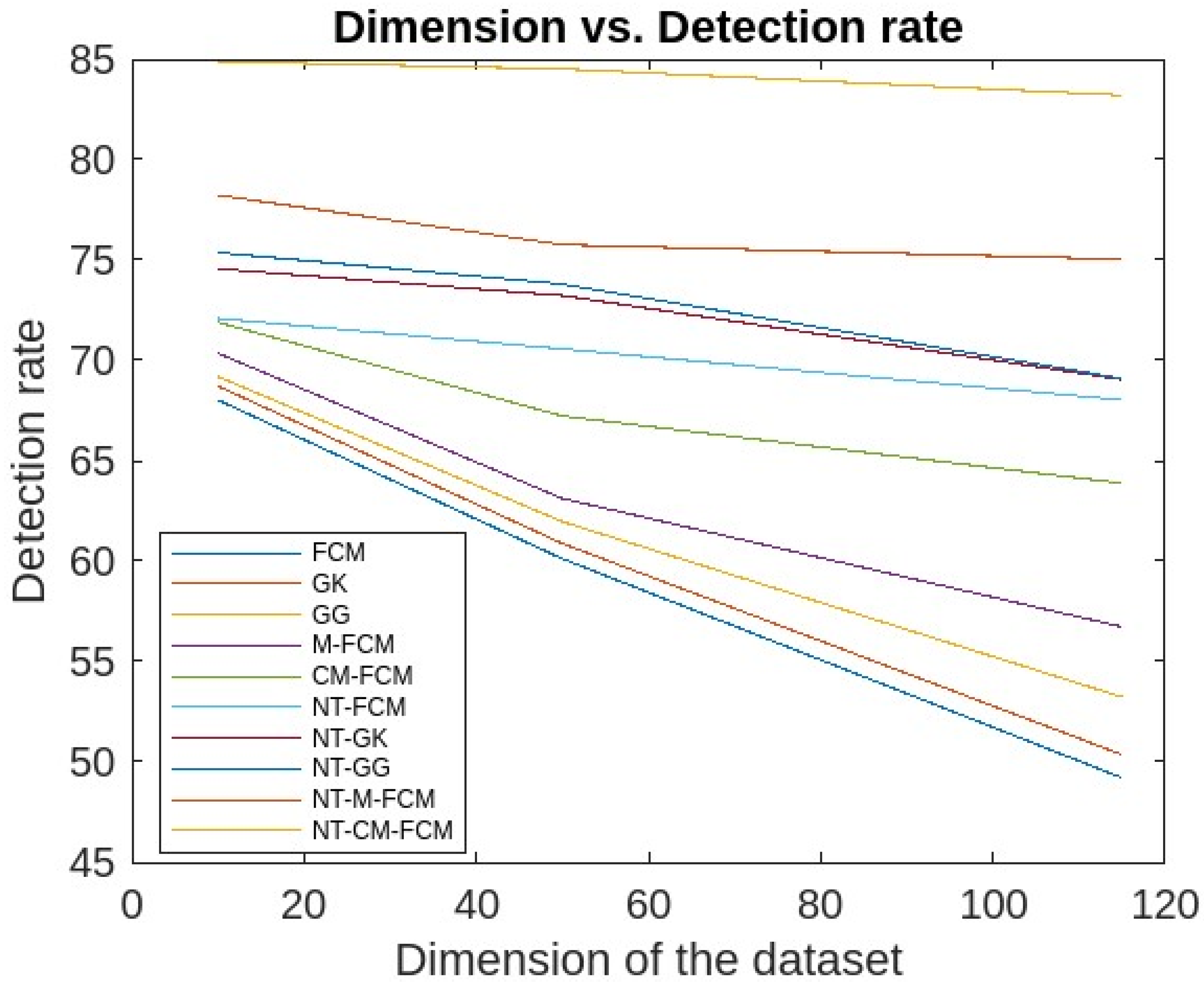
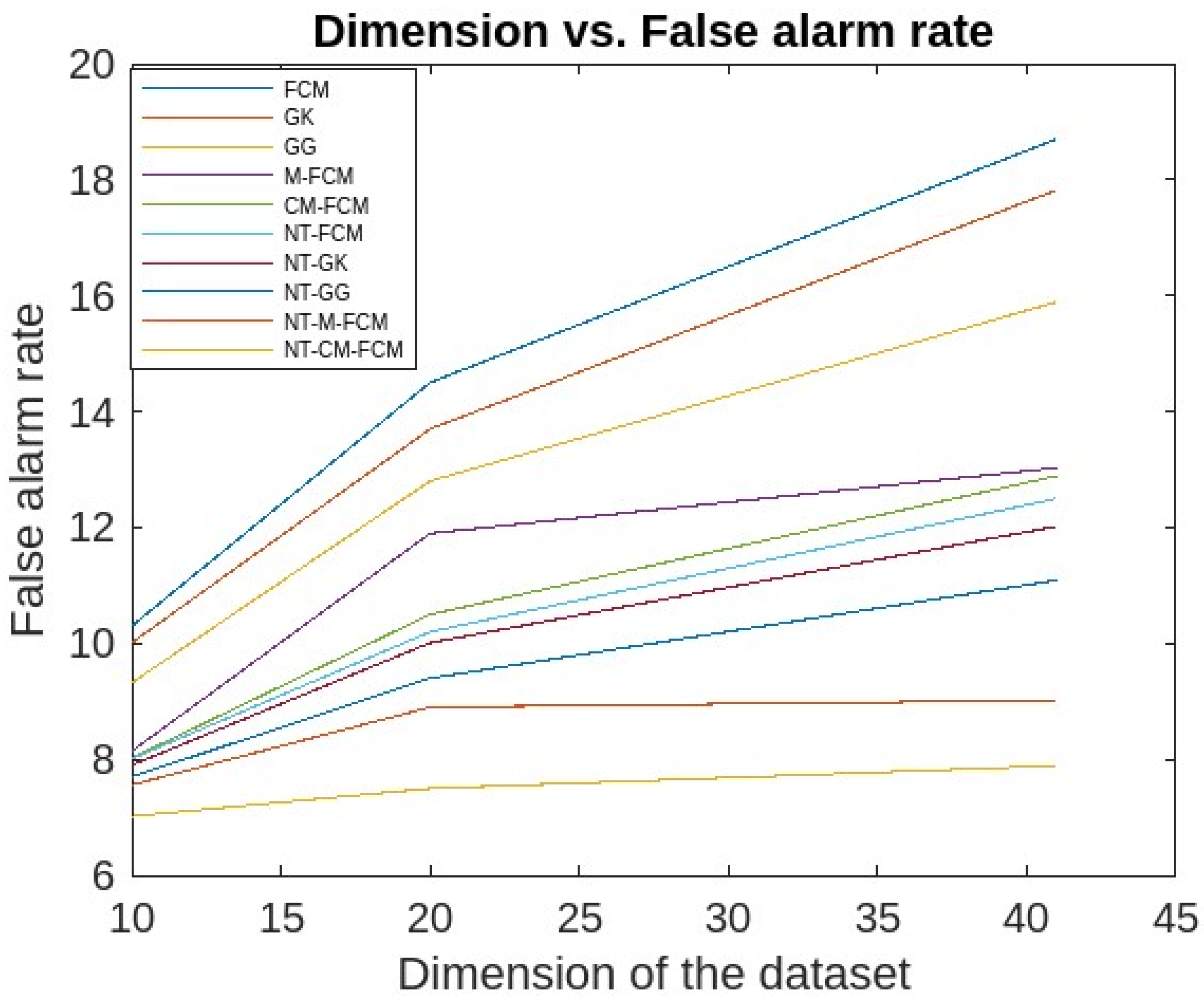
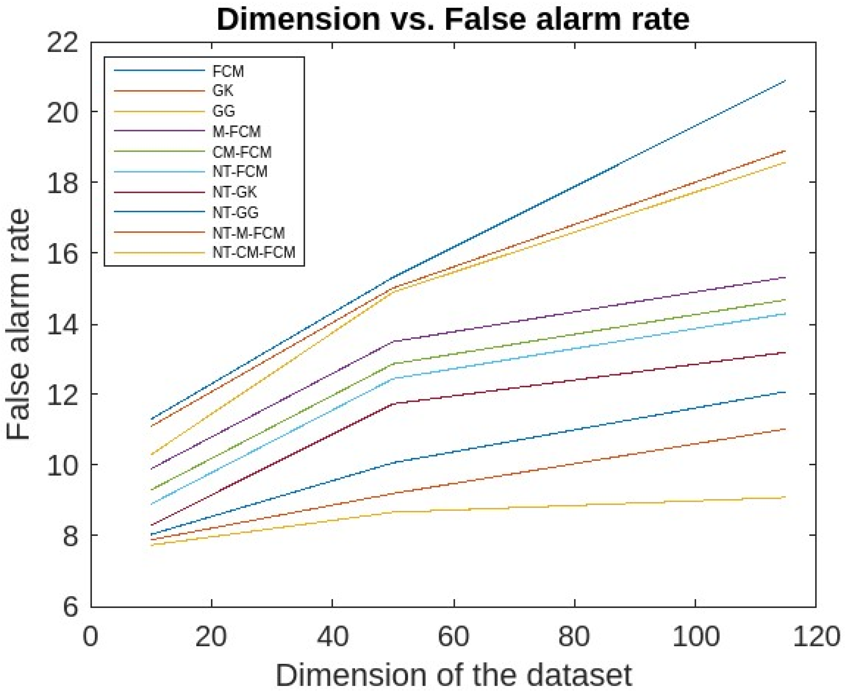
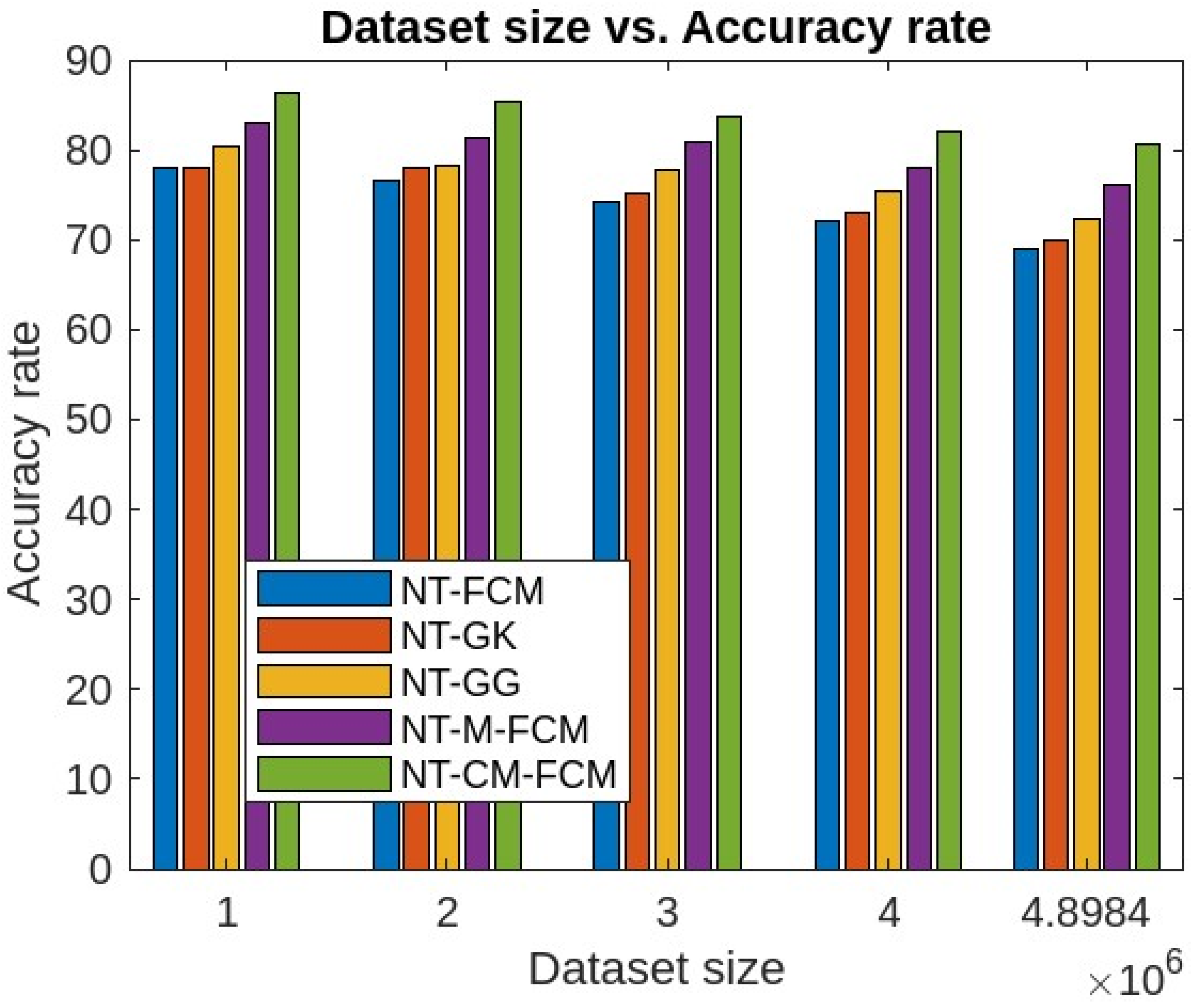
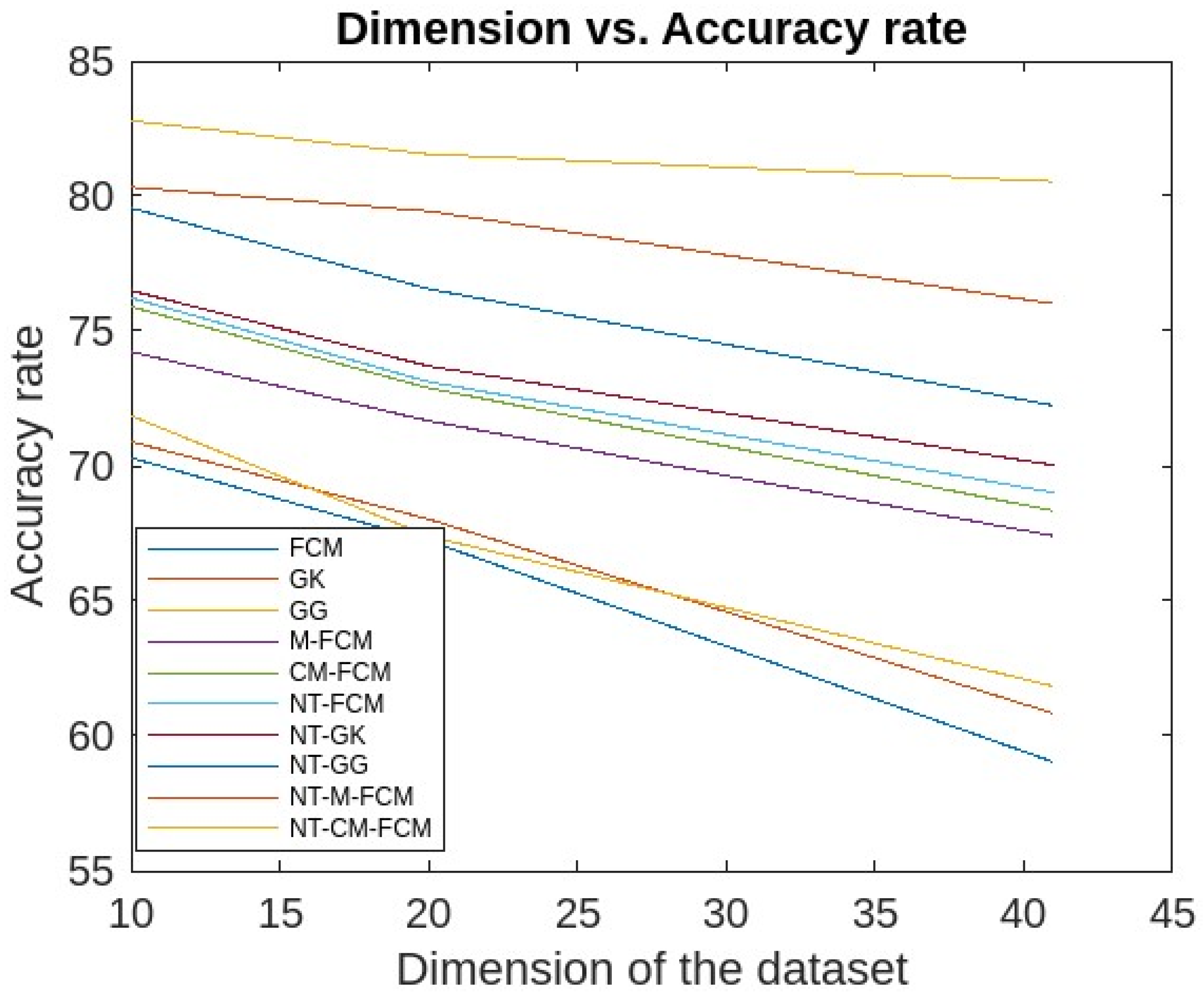
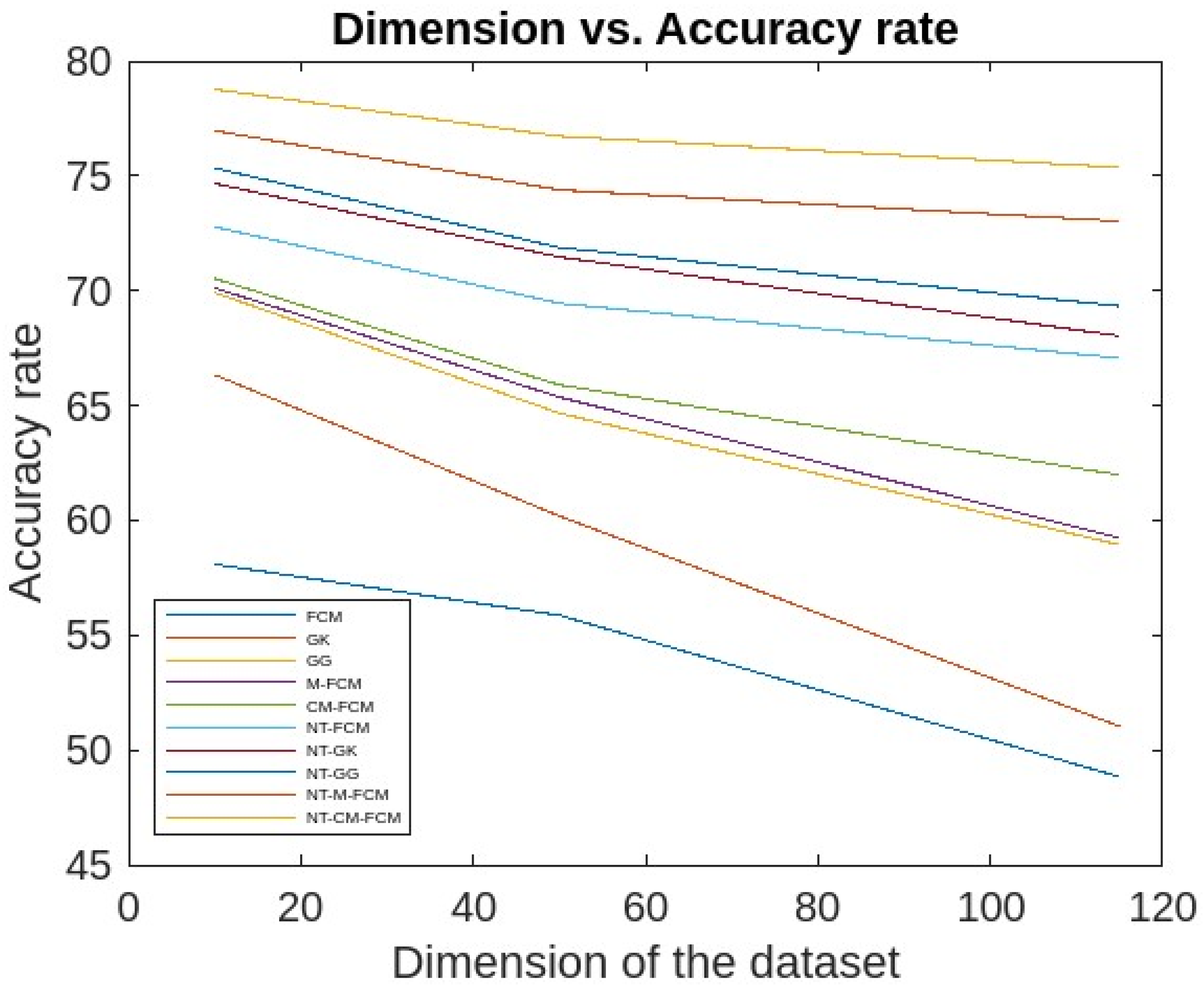
5.1. Experimental Analysis and Results

For testing the efficacy of the approaches employed here, two well-known datasets, namely, the KDDCup’99 Network Anomaly dataset [50] and Kitsune Network Attack dataset [51], are used. The detailed descriptions of the datasets are given below.

KDD CUP’99 [50]: It is a synthetic dataset that simulates intrusion in the military network environment. The data are collected for 9 weeks, and its training data consist of 5 million network connections. The attributes can be divided into the classes, viz., normal (unauthorized access to local super user privileges, unauthorized access from a remote machine), dos, and probe.

Kitsune [51]: It is a group of nine network attack datasets, each containing millions of network packets and different cyberattacks, which were either gathered from an IP-based commercial surveillance system or a network of IoT devices.

The datasets are obtained from the UCI machine repository. The datasets along with their characteristics in summarized form are described in

Table 1. Dataset descriptions.

Dataset	Dataset Characteristics	Attribute Characteristics	No. of Instances	No. of Attributes
KDDCup’99 [50]	Synthetic, Multivariate	Numeric, categorical, and temporal	4,898,431	41
Kitsune Network Attack [51]	Real-life, Multivariate, sequential, time-series	Real, temporal	27,170,754	115

below.

The experiments were conducted on a standard machine using two datasets described in Table 1. With the KDDCup’99 [50], two datasets, one having different sizes but fixed dimensions and the other having fixed sizes and different dimensions, are constructed. Similarly, with the Kitsune dataset [51], two datasets of similar sizes are constructed. The proposed methods, namely NT-FCM, NT-GK, NT-GG, NT-M-FCM, and NT-CM-FCM, are implemented using MATLAB with the aforesaid four constructed datasets. The comparative analysis of the proposed approaches along with traditional fuzzy clustering algorithms, namely FCM [41], GK [42], GG [43], M-FCM [47], and CM-FCM [47], are conducted. Further, the performances of the proposed methods along with traditional fuzzy clustering algorithms are studied in manifolds, like accuracies in detection rates, the percentage of anomalies obtained, percentage of false alarm rates, etc. The detailed findings of the aforesaid investigations are presented both in tabular form in

Table 2. Relative analysis of detection of FCM, GK, GG, M-FCM, and CM-FCM rate using two datasets (dimension of dataset is constant).

Performances of FCM, GK, GG, M-FCM, Using the Two Datasets
Datasets		FCM	GK	GG	M-FCM	CM-FCM
KDDCup’99	Detection rate	60.3	62.06	65.3	66.03	72.08
	Accuracy rate	59.03	60.83	61.84	67.41	68.34
	False alarm rate	18.7	17.82	15.89	13.03	12.89
	Denial of service	69.63	72.73	75.02	78.85	87.32
	Remote to local	68.87	73.02	73.99	76.82	81.21
	User to root	42.60	50.79	52.21	54.98	61.31
	Probe	51.47	56.35	53.98	57.88	61.13
Kitsune dataset	Detection rate	49.21	50.36	53.23	56.73	63.88
	Accuracy rate	48.83	51.03	58.94	59.23	61.98
	False alarm rate	20.9	18.92	18.59	15.33	14.69
	Denial of service	67.83	71.63	73.72	80.25	84.32
	Remote to local	66.7	71.42	71.89	73.92	80.31
	User to root	40.90	49.29	50.91	52.77	60.91
	Probe	50.07	54.95	54.87	56.78	60.34

,

Table 3. Comparative analysis of various attack parameters using KDDCup’99.

% of Attack Parameters
Sl. NO.	Parameters	NT-FCM	NT-GK	NT-GG	NT-M-FCM	NT-CM-FCM
1	Denial of service	79.73	83.33	84.92	89.95	96.22
2	Remote to local	78.56	82.42	83.85	85.72	90.40
3	User to root	52.40	60.39	61.70	65.90	70.81
4	Probe	62.37	65.45	64.65	68.81	70.73

and

Table 4. Comparative analysis of various attack parameters using Kitsune dataset.

% of Attack Parameters
Sl. NO.	Parameters	NT-FCM	NT-GK	NT-GG	NT-M-FCM	NT-CM-FCM
1	Denial of service	78.3	81.33	82.99	87.96	94.83
2	Remote to local	77.56	81.42	81.85	82.83	90.22
3	User to root	53.50	58.89	60.80	63.89	68.91
4	Probe	61.79	64.53	63.75	66.91	69.84

and graphically in Figure 6, Figure 7, Figure 8, Figure 9, Figure 10, Figure 11, Figure 12, Figure 13, Figure 14, Figure 15, Figure 16, Figure 17, Figure 18 and Figure 19 below.

Table 2 gives the performances of the traditional fuzzy clustering algorithms FCM, GK, GG, M-FCM, and CM-FCM with the datasets KDDCup’99 [50] and Kitsune [51]. The dimension of the two datasets is assumed to be constant. The performances are measured using the parameters like detection rate, accuracy rate, false alarm rate, denial of service, remote to local, and probe. It has been observed from the table that the CM-FCM clustering algorithm outperforms others in all the parameters and its performance is the best in the case of the KDDCup’99 [50] dataset.

The above figure gives the detection rates of all the five NT-based fuzzy clustering methods with different sizes of the dataset KDDCup’99 [50]. The dataset sizes considered are 1,000,000, 2,000,000, 3,000,000, 4,000,000, and 4,898,431 records. The dimension of the dataset is taken as a constant. The methods are executed multiple times with the given sizes of the dataset, and the corresponding results are recorded and presented as a bar diagram in Figure 6.

Figure 7 gives the accuracy rates of all the five NT-based fuzzy clustering methods with different sizes of the dataset KDDCup’99 [50]. Similar to the previous figure, dataset sizes considered are 1,000,000, 2,000,000, 3,000,000, 4,000,000, and 4,898,431 records, and the dimension of the dataset is taken as a constant. The methods are executed multiple times for the given sizes of the dataset, and the corresponding accuracy rates are recorded and presented as a bar diagram in Figure 7.

Figure 8 displays the false alarm rates of all the five NT-based fuzzy clustering methods with different sizes of the dataset KDDCup’99 [50]. Similar to the detection and accuracy rates, the dataset sizes considered and the dimension of the dataset are taken as constants. The methods are executed multiple times with the given dataset sizes, and the corresponding false alarm rates are recorded and presented as a bar diagram in Figure 8.

Table 3 presents the results obtained in terms of four attack parameters, namely denial of service, remote to local, user to root, and probe by NT-FCM, NT-GK, NT-GG, NT-M-FCM, and NT-CM-FCM clustering algorithms in tabular form. The dataset used here is KDDCup’99 [50]. It can easily be seen in the table that NT-CM-FCM outperforms the others, and the performances of the methods decreases from right to left.

Figure 9 presents the results of Table 3 in a convenient way using a bar diagram. The algorithm NT-FCM is the least efficient, and NT-CM-FCM is the most efficient in terms of percentage of attack parameters.

Figure 10 gives the detection rates of all the five NT-based fuzzy clustering methods with different sizes of the Kitsune dataset [51]. The dataset sizes considered are 1,000,000, 5,000,000, 10,000,000, 15,000,000, and 27,170,754 records, and the dimension of the dataset is assumed to be constant. The methods are executed a couple of times with the different sizes of the dataset, and the corresponding results are recorded and displayed as a bar diagram in Figure 10.

Figure 11 gives the accuracy rates of all the five NT-based fuzzy clustering methods with different sizes of the Kitsune dataset [51]. The dataset sizes considered are 1,000,000, 5,000,000, 10,000,000, 15,000,000, and 27,170,754 records, and the dimension of the dataset is assumed to be constant. The methods are executed multiple times with these features of the dataset, and the corresponding results are recorded and displayed as a bar diagram in Figure 11.

Figure 12 gives the false alarm rates of all the five NT-based fuzzy clustering methods with different sizes of the Kitsune dataset [51]. The dataset sizes considered are 1,000,000, 5,000,000, 10,000,000, 15,000,000, and 27,170,754 records, and the dimension of the dataset is assumed to be constant. The methods are executed multiple times with these sizes of the dataset, and the corresponding results are recorded and displayed as a bar diagram in Figure 12.

Table 4 presents results obtained in terms of four attack parameters, namely denial of service, remote to local, user to root, and probe, by NT-FCM, NT-GK, NT-GG, NT-M-FCM, and NT-CM-FCM clustering algorithms in tabulated form. The dataset used here is the Kitsune dataset [51]. From the table, similar observations can be drawn that NT-CM-FCM outperforms the others, and the performances of the methods decreases from right to left.

Figure 13 presents the results of Table 4 in a convenient way using a bar diagram. Similar to Table 3 and Figure 9, it can be observed here that the algorithm NT-FCM is the least efficient, and NT-CM-FCM is the most efficient in terms of the percentage of attack parameters.

Figure 14 gives the detection rates of both traditional as well as NT-based fuzzy clustering methods with respect to the dimensions of the KDDCup’99 [50]. For the different experiments, the dimensions of the dataset are taken as 10, 20, and 41. The methods are executed as many times as the set of dimensions of the dataset, and the corresponding results in terms of detection rates are recorded and displayed graphically in Figure 14.

Figure 15 presents the detection rates of both traditional as well as NT-based fuzzy clustering methods with respect to the dimensions of the Kitsune dataset [51]. For the different experiments, the dimensions of the dataset are taken as 10, 50, and 115. The methods are executed as many times as the set of dimensions of the dataset, and the corresponding results in terms of detection rates are recorded and displayed graphically in Figure 15.

The above figure gives the accuracy rates of both traditional as well as NT-based fuzzy clustering methods with respect to the dimensions of the KDDCup’99 [50]. For the different experiments, the dimensions of the dataset are taken as 10, 20, and 41. The methods are executed as many times as the set of dimensions of the dataset, and the corresponding results in terms of accuracy rates are recorded and displayed graphically in Figure 16.

The above figure presents the accuracy rates of both traditional as well as NT-based fuzzy clustering methods with respect to the dimensions of the Kitsune dataset [51]. For the different experiments, the dimensions of the dataset are taken as 10, 50, and 115. The methods are executed as many times as the set of dimensions of the dataset, and the corresponding results in terms of accuracy rates are recorded and displayed graphically in Figure 17.

The above figure gives the false alarm rates of both traditional as well as NT-based fuzzy clustering methods with respect to the dimensions of the KDDCup’99 [50]. For the different experiments, the dimensions of the dataset are taken as 10, 20, and 41. The methods are executed as many times as the set of dimensions of the dataset, and the corresponding results in terms of false alarm rates are recorded and displayed graphically in Figure 18.

The above figure presents the false alarm rates of both traditional as well as NT-based fuzzy clustering methods with respect to the dimensions of the Kitsune dataset [51]. For the different experiments, the dimensions of the dataset are taken as 10, 50, and 115. The methods are executed as many times as the set of dimensions of the dataset, and the corresponding results in terms of false alarm rates are recorded and displayed graphically in Figure 19.

5.2. Discussions

The following inferences can be drawn from the obtained results. Table 2 presents the detection rates, the accuracy rates, the false alarm rates, and all the four attack parameters (denial of service, remote to local, user to root, and probe) of FCM, GK, GG, M-FCM, and CM-FCM with the two datasets, KDDCup’99 [50] and Kitsune [51]. It is evident from Table 2 that among all the aforesaid traditional fuzzy clustering algorithms, the CM-FCM performs the best, and performances follow the following order: CM-FCM, M.FCM, GG, GK, and FCM. It is evident from the results of the Kitsune dataset [51], which is much larger than KDDCup’99 [50], that the performances of the above algorithms reduce rapidly when a comparatively larger dataset is considered, which means that the performances of the traditional fuzzy clustering algorithms depend both on the size and dimension of the dataset.

The bar diagrams in Figure 6 and Figure 10 represent the detection rates of the five NT-based fuzzy clustering algorithms for KDDCup’99 [50] and Kitsune [51], respectively. It can be seen in the bar diagram that the anomaly detection rates of all of the algorithms improve if the NT-based subspace clustering approach is considered. With KDDCup’99 [50], the NT-CM-FCM performs best with the detection rate of 91.3%, and NT-FCM performs worst with 82.6%, which is far better than the traditional CM-FCM’s detection rate (72.08%). Similarly, with the comparatively larger dataset of Kitsune [51], the NT-CM-FCM performs best with the detection rate of 90.8%, and NT-FCM performs the worst with 78.5%. A similar observation can be made for other NT-based methods. Also, the detection rate decreases with the increase in the size of the dataset, but the rate of decrease is much slower. Both results show that the detection rates of NT-based approaches depend little on the sizes and the dimensions of the datasets. The detection rates of NT-based algorithms follow the order NT-CM-FCM, NT-M-FCM, GG, GK, and FCM. Also, there exists a linear relationship between the detection rate of each NT-based approach and the dataset size.

As far as the accuracy of anomaly detection is concerned, Figure 7 and Figure 11 and their descriptions show that the NT-based approach of the fuzzy clustering algorithms performs impressively in comparison to the traditional fuzzy clustering approaches. Similar to the detection rate, the accuracy rate decreases visibly less with respect to the increment of the dataset size, which means that there is a linear relationship between the accuracy rate of each NT-based approach and the dataset size. The NT-CM—FCM is found to be comparatively better as its accuracy of anomaly detection ranges from 80.54% to 86.5% for the KDDCup’99 [50] dataset and from 75.37% to 82.6% for the Kitsune dataset [51]. The accuracy rate follows ascending order from left to right in the case of both datasets.

From Figure 8 and Figure 12, it is evident that the false alarm rates of NT-based algorithms are quite lesser than the traditional fuzzy clustering algorithms, and also the false alarm rate of NT-CM-FCM is comparatively much better than the others. With the KDDCup’99 [50], the false alarm rate of the NT-CM-FCM algorithm ranges between 3.78 and 7.89% with respect to the data size range of 1,000,000–4,898,431, and with the Kitsune dataset [51], it ranges from 5.8 to 9.09% with respect to the data size of range 1,000,000–27,170,754. It is also evident from the results that the false alarm rate is more or less uniform with respect to data size, i.e., the relationship is linear. Furthermore, the false alarm rate follows descending order from left to right in the case of both datasets.

In Table 2, Table 3 and Table 4 and Figure 9 and Figure 13, the percentage of different attack parameters (denial of service, remote to local, user to root, and probe) are presented. For example, the percentage of denial of service of the ten algorithms (traditional and NT-based) are, respectively, 69.63, 72.73, 75.02, 78.85, 87.32, 79.73, 83.33, 84.92, 89.95, and 96.22. From these results, some interesting observations can be made; for instance, the traditional CM-FCM performance is better than NT-FCM, NT-GK, and NT-GG. This means that the algorithm CM-FCM, whether traditional or NT-based, outperforms all of the other algorithms, and the NT-CM-FCM algorithm is the best among all. Also, in case of the attack parameter, remote to local, CM-FCM performs better than NT-FCM, and NT-CM-FCM outperforms others. Similar observations can be made for the other two attack parameters (user to root and probe). From the above discussions, it can be concluded that the dimension reduction has little impact on the attack parameters of the algorithm CM-FCM, as the performances of CM-FCM and NT-CM-FCM are almost the same.

From Figure 14 and Figure 15, it can be inferred that for different sizes (the dimensions sizes are taken as 10, 20 and 41) of the dimensions of the KDDCup’99 [50], the detection rate ranges of FCM, GK, GG, M-FCM, CM-FCM, NT-FCM, NT-GK, NT-GG, NT-M-FCM, and NT-CM-FCM are, respectively, 60.3–72.34, 62.06–75.56, 65.3–77.01, 66.03–77.45, 72.08–83.05, 72.1–75.78, 73.05–76.01, 74.1–76.3, 76.02–80.2, and 84.02–85.3, and for the dimensions of 10, 50 and 115, in the Kitsune dataset [51], the ranges are 49.21–68.03, 50.36–68.72, 53.23–69.19, 56.73–70.36, 63.88–71.9, 68.03–72.09, 69.05–74.56, 69.1–75.37, 75.04–78.23, and 83.21–84.89. It can be inferred from the data that for a lower dimensional dataset, most of the algorithms work nicely, even M-FCM and CM-FCM’s efficacy of anomaly detection is higher than some of the NT-based approaches like NT-FCM and NT-GK. However, when the dimension increases, the detection rates of all of the traditional fuzzy clustering algorithms fall rapidly and those of the NT-based approaches fall consistently. Thus, the NT-based algorithms perform better comparatively, which also shows that NT-based algorithms are less dependent on the dimension of the datasets. It is to be mentioned here that algorithms NT-M-FCM and NT-CM-FCM’s anomaly detection rates are much better than the others.

Figure 16 and Figure 17 give the accuracy rates of detection for all the aforesaid ten algorithms e, respectively, as 59.03–70.3, 60.83–70.9, 61.84–71.86, 67.41–74.23, 68.34–75.9, 69.01–76.23, 70.03–76.5, 72.24–79.56, 76.01–80.33, and 80.54–82.79 for the dataset KDDCup’99 [50] (the dimensions sizes are taken as 10, 20, and 41) and as 48.83–58.09, 51.03–66.34, 58.94–69.92, 59.23–70.12, 61.98–70.53, 67.07–72.78, 68.03–74.67, 69.33–75.34, 73.03–76.97, and 75.37–78.77 for the dataset Kitsune [51] (the dimensions sizes are taken as 10, 50, and 115). Since the accuracy ranges more for the traditional fuzzy clustering algorithms than the NT-based algorithms, which in turn, established the fact that later algorithms are less dependent on the sizes of dimensions of the datasets. It is to be mentioned here that NT-CM-FCM is comparatively better than the others in terms of the accuracy rate of anomaly detection.

The false alarm rates of the aforesaid algorithms for the different dimensions of the KDDCup’99 [50] dataset have respective ranges of 10.3–18.7, 10.01–17.82, 9.32–15.89, 8.14–13.03, 8.02–12.89, 8.01–12.5, 7.9–12.02, 7.7–11.09, 7.56–9.02, and 7.02–7.89, and for the Kitsune dataset [51], respective ranges are 20.9–11.3, 18.92–11.1, 18.59–10.3, 15.33–9.9, 14.69–9.3, 14.3–8.9, 13.2–8.3, 12.09–8.04, 11.03–7.89, and 9.09–7.74, which is evident from Figure 18 and Figure 19. It has been observed that the false alarm rates of all of the algorithms increases with the increase in the dimension of the datasets. However, for the NT-based algorithms, the rate of increase is comparatively slower, and NT-CM-FCM is the slowest. It is also observed that the rates of decrease are from left to right, which shows that NT-CM-FCM is the best among all of the algorithms, whether traditional or NT-based.

Furthermore, Figure 14 shows the relationship of the detection rates with the dimensions of KDDCup’99 [50]. It can be seen from Figure 14, Figure 16 and Figure 18 that all of the five traditional fuzzy clustering algorithms, namely FCM, GK, GG, M-FCM, CM-FCM, perform in terms of detection rates, accuracy rates, and false alarm rates very well in the lower dimensional spaces, but performances decrease rapidly with the increase in dimensions. The rate of decrease is very fast initially, though it appears to be a little better later. So, it appears that the traditional fuzzy clustering algorithms show inconsistent behavior with respect to the dimension of the dataset. However, the proposed algorithms, especially NT-CM-FCM, perform uniformly in all parameters. Also, in the case of other NT-based approaches, the results are more or less consistent. This means that the NT-based approaches have consistent relationships with the dimension of the KDDCup’99 [50] datasets. In the case of the Kitsune dataset [51], similar observations can be made. From Figure 15, Figure 17 and Figure 19, similar findings are observed, i.e., the NT-based approaches maintain consistency with the dimensions of both the dataset in all of the performance parameters like accuracy rate, false alarm rate, etc. However, the traditional approaches are non-uniform, and they show multiple linear relationships. The NT-CM-FCM fuzzy clustering algorithm shows the most consistent performance in all of the given parameters.

6. Conclusions, Limitations, and Lines for Future Works

6.1. Conclusions

In this article, two-phased methods of fuzzy subspace clustering for anomaly detections were proposed. The input dataset is initially transformed into a set-valued information system using the rough set theoretic approach, which establishes a dominance relation on it. Then, a nano topology, along with its basis, is constructed by removing insignificant attributes of the dataset. The constructed nano topology creates a lower dimensional space of the original dataset. In the second phase, fuzzy clustering algorithms were employed for anomaly detections. For fuzzy clustering, the traditional algorithms like FCM [41], GK [42,47], GG [43,47], M-FCM [47], and CM-FCM [47] were used. The proposed algorithms are named NT-FCM, NT-GK, NT-GG, NT-M-FCM, and NT-CM-FCM. Each of the proposed methods supplies a specified number of fuzzy clusters. The data instance not belonging to any of the clusters or belonging to a minimum membership value can be treated as an anomaly. The efficacies of the proposed approaches were studied by experimental analysis on a synthetic dataset, KDDCup’99 [50], and a real-life dataset, Kitsune [51], and comparative studies have been made with the traditional fuzzy clustering approaches and among the proposed approaches. The results showed that the NT-based algorithms outperform the traditional approaches in all of the parameters like detection rate, accuracy rate, false alarm rate, and run-time complexities.

Though among all the aforesaid methods, NT-CM-FCM is the best, its traditional algorithm CM-FCM sometimes performs better than the other NT-based fuzzy clustering approaches.

Finally, any NT-based method is a combination of two algorithms where Algorithm 1 returns subspaces of the datasets. So, the run-time complexity of Algorithm 1 depends on the data size and dimensions. It is quadratic to the dataset size and linear to the dimension. Since the size of any dataset is bigger than its dimension size, and the dimension size of the subspace is quite small, the time complexity of all of the NT-based algorithms depends on the time complexity of Algorithm 1 and the dataset size. It has been found that the NT-M-FCM and NT-CM-FCM run in cubic time, but the others run in biquadratic time.

6.2. Limitations and Lines for Future Works

Though the NT-based approaches are performing better than the traditional fuzzy clustering approaches, they are not free from limitations. Firstly, through using Algorithm 1, the computational cost of any NT-based algorithm can be reduced up to some extent, but they are still more expensive than non-fuzzy clustering, as they require optimization over multiple membership grades. Secondly, choosing the number of clusters and membership functions is the most challenging task which requires either trial/error approach or a domain expert.

The future lines of work can be focused on the following.

• In the future, the time attribute can be addressed separately to find fuzzy clusters along with lifetimes which may provide detailed insights of the IoT system.
• In the future, detecting anomalies from high-dimensional data may be accomplished with an effective supervised approach.

References

- Sethi, P.; Sarangi, S. Internet of things: Architectures, protocols, and applications. J. Electr. Comput. Eng. 2017, 2017, 9324035. [Google Scholar] [CrossRef]
- Erfani, S.M.; Rajasegarar, S.; Karunasekera, S.; Leckie, C. High-dimensional and large-scale anomaly detection using a linear one-class SVM with deep learning. Pattern Recogn. 2016, 58, 121–134. [Google Scholar] [CrossRef]
- Hodge, V.; Austin, J. A survey of outlier detection methodologies. Artif. Intell. Rev. 2004, 22, 85–126. [Google Scholar] [CrossRef]
- Hartigan, J.A. Clustering Algorithms; John Wiley & Sons: Hoboken, NJ, USA, 1975. [Google Scholar]
- Aggarwal, C.C.; Philip, S.Y. An effective and efficient algorithm for high-dimensional outlier detection. VLDB J. 2005, 14, 211–221. [Google Scholar] [CrossRef]
- Ramchandran, A.; Sangaiah, A.K. Chapter 11—Unsupervised Anomaly Detection for High Dimensional Data—An Exploratory Analysis, Computational Intelligence for Multimedia Big Data on the Cloud with Engineering Applications. In Intelligent Data-Centric Systems; Academic Press: Cambridge, MA, USA, 2018; pp. 233–251. [Google Scholar]
- Pawlak, Z. Rough sets. Int. J. Comput. Inf. Sci. 1982, 11, 341–356. [Google Scholar] [CrossRef]
- Mazarbhuiya, F.A. Detecting Anomaly using Neighborhood Rough Set based Classification Approach. ICIC Express Lett. 2023, 17, 73–80. [Google Scholar]
- Thivagar, M.L.; Richard, C. On nano forms of weakly open sets. Int. J. Math. Stat. Invent. 2013, 1, 31–37. [Google Scholar]
- Thivagar, M.L.; Priyalatha, S.P.R. Medical diagnosis in an indiscernibility matrix based on nano topology. Cogent Math. 2017, 4, 1330180. [Google Scholar] [CrossRef]
- Mung, G.; Li, S.; Carle, G. Traffic Anomaly Detection Using k-Means Clustering; Allen Institute for Artificial Intelligence: Seattle, WA, USA, 2007. [Google Scholar]
- Ren, W.; Cao, J.; Wu, X. Application of network intrusion detection based on fuzzy c-means clustering algorithm. In Proceedings of the 3rd International Symposium on Intelligent Information Technology Application, Nanchang, China, 21–22 November 2009; pp. 19–22. [Google Scholar]
- Mazarbhuiya, F.A.; AlZahrani, M.Y.; Georgieva, L. Anomaly detection using agglomerative hierarchical clustering algorithm. In Lecture Notes in Electrical Engineering; Springer: Singapore, 2018. [Google Scholar] [CrossRef]
- Mazarbhuiya, F.A.; AlZahrani, M.Y.; Mahanta, A.K. Detecting Anomaly Using Partitioning Clustering with Merging. ICIC Express Lett. 2020, 14, 951–960. [Google Scholar]
- Retting, L.; Khayati, M.; Cudre-Mauroux, P.; Piorkowski, M. Online anomaly detection over Big Data streams. In Proceedings of the 2015 IEEE International Conference on Big Data, Santa Clara, CA, USA, 29 October–1 November 2015. [Google Scholar]
- The, H.Y.; Wang, K.I.; Kempa-Liehr, A.W. Expect the unexpected: Un-supervised feature selection for automated sensor anomaly detection. IEEE Sens. J. 2021, 21, 18033–18046. [Google Scholar] [CrossRef]
- Alguliyev, R.; Aliguliyev, R.; Sukhostat, L. Anomaly Detection in Big Data based on Clustering. Stat. Optim. Inf. Comput. 2017, 5, 325–340. [Google Scholar] [CrossRef]
- Hahsler, M.; Piekenbrock, M.; Doran, D. dbscan: Fast Density-based clustering with R. J. Stat. Softw. 2019, 91, 1–30. [Google Scholar] [CrossRef]
- Song, H.; Jiang, Z.; Men, A.; Yang, B. A Hybrid Semi-Supervised Anomaly Detection Model for High Dimensional data. Comput. Intell. Neurosci. 2017, 2017, 8501683. [Google Scholar] [CrossRef] [PubMed]
- Mazarbhuiya, F.A. Detecting IoT Anomaly Using Rough Set and Density Based Subspace Clustering. ICIC Express Lett. 2023, 17, 1395–1403. [Google Scholar] [CrossRef]
- Alghawli, A.S. Complex methods detect anomalies in real time based on time series analysis. Alex. Eng. J. 2022, 61, 549–561. [Google Scholar] [CrossRef]
- Younas, M.Z. Anomaly Detection using Data Mining Techniques: A Review. Int. J. Res. Appl. Sci. Eng. Technol. 2020, 8, 568–574. [Google Scholar] [CrossRef]
- Thudumu, S.; Branch, P.; Jin, J.; Singh, J. A comprehensive survey of anomaly detection techniques for high dimensional big data. J. Big Data 2020, 7, 42. [Google Scholar] [CrossRef]
- Habeeb, R.A.A.; Nasauddin, F.; Gani, A.; Hashem, I.A.T.; Ahmed, E.; Imran, M. Real-time big data processing for anomaly detection: A Survey. Int. J. Inf. Manag. 2019, 45, 289–307. [Google Scholar] [CrossRef]
- Wang, B.; Hua, Q.; Zhang, H.; Tan, X.; Nan, Y.; Chen, R.; Shu, X. Research on anomaly detection and real-time reliability evaluation with the log of cloud platform. Alex. Eng. J. 2022, 61, 7183–7193. [Google Scholar] [CrossRef]
- Halstead, B.; Koh, Y.S.; Riddle, P.; Pechenizkiy, M.; Bifet, A. Combining Diverse Meta-Features to Accurately Identify Recurring Concept Drit in Data Streams. ACM Trans. Knowl. Discov. Data 2023, 17, 1–36. [Google Scholar] [CrossRef]
- Zhao, Z.; Birke, R.; Han, R.; Robu, B.; Bouchenak, S.; Ben Mokhtar, S.; Chen, L.Y. RAD: On-line Anomaly Detection for Highly Unreliable Data. arXiv 2019, arXiv:1911.04383. [Google Scholar]
- Chenaghlou, M.; Moshtaghi, M.; Lekhie, C.; Salahi, M. Online Clustering for Evolving Data Streams with Online Anomaly Detection. Advances in Knowledge Discovery and Data Mining. In Proceedings of the 22nd Pacific-Asia Conference, PAKDD 2018, Melbourne, VIC, Australia, 3–6 June 2018; pp. 508–521. [Google Scholar]
- Firoozjaei, M.D.; Mahmoudyar, N.; Baseri, Y.; Ghorbani, A.A. An evaluation framework for industrial control system cyber incidents. Int. J. Crit. Infrastruct. Prot. 2022, 36, 100487. [Google Scholar] [CrossRef]
- Chen, Q.; Zhou, M.; Cai, Z.; Su, S. Compliance Checking Based Detection of Insider Threat in Industrial Control System of Power Utilities. In Proceedings of the 2022 7th Asia Conference on Power and Electrical Engineering (ACPEE), Hangzhou, China, 15–17 April 2022; pp. 1142–1147. [Google Scholar]
- Zhao, Z.; Mehrotra, K.G.; Mohan, C.K. Online Anomaly Detection Using Random Forest. In Recent Trends and Future Technology in Applied Intelligence; Mouhoub, M., Sadaoui, S., Ait Mohamed, O., Ali, M., Eds.; IEA/AIE 2018; Lecture Notes in Computer Science; Springer: Cham, Switzerland, 2018. [Google Scholar]
- Izakian, H.; Pedrycz, W. Anomaly detection in time series data using fuzzy c-means clustering. In Proceedings of the 2013 Joint IFSA World Congress and NAFIPS Annual Meeting, Edmonton, AB, Canada, 24–28 June 2013. [Google Scholar]
- Decker, L.; Leite, D.; Giommi, L.; Bonakorsi, D. Real-time anomaly detection in data centers for log-based predictive maintenance using fuzzy-rule based approach. arXiv 2020, arXiv:2004.13527v1. Available online: https://arxiv.org/pdf/2004.13527.pdf (accessed on 15 March 2022).
- Masdari, M.; Khezri, H. Towards fuzzy anomaly detection-based security: A comprehensive review. Fuzzy Optim. Decis. Mak. 2020, 20, 1–49. [Google Scholar] [CrossRef]
- de Campos Souza, P.V.; Guimarães, A.J.; Rezende, T.S.; Silva Araujo, V.J.; Araujo, V.S. Detection of Anomalies in Large-Scale Cyberattacks Using Fuzzy Neural Networks. AI 2020, 1, 92–116. [Google Scholar] [CrossRef]
- Talagala, P.D.; Rob, J. Hyndman, and Kate Smith-Miles, Anomaly Detection in High-Dimensional Data. J. Comput. Graph. Stat. 2021, 30, 360–374. [Google Scholar] [CrossRef]
- Al Samara, M.; Bennis, I.; Abouaissa, A.; Lorenz, P. A Survey of Outlier Detection Techniques in IoT: Review and Classification. J. Sens. Actuator Netw. 2022, 11, 4. [Google Scholar] [CrossRef]
- Yugandhar, A.; Sashirekha, S.K. Dimensional Reduction of Data for Anomaly Detection and Speed Performance using PCA and DBSCAN. Int. J. Eng. Adv. Technol. 2019, 9, 39–41. [Google Scholar]
- Mazarbhuiya, F.A.; Shenify, M. A Mixed Clustering Approach for Real-Time Anomaly Detection. Appl. Sci. 2023, 13, 4151. [Google Scholar] [CrossRef]
- Mazarbhuiya, F.A.; Shenify, M. Real-time Anomaly Detection with Subspace Periodic Clustering Approach. Appl. Sci. 2023, 13, 7382. [Google Scholar] [CrossRef]
- Harish, B.S.; Kumar, S.V.A. Anomaly based Intrusion Detection using Modified Fuzzy Clustering. Int. J. Interact. Multimed. Artif. Intell. 2017, 4, 54–59. [Google Scholar] [CrossRef]
- Gustafson, D.E.; Kessel, W. Fuzzy clustering with a fuzzy covariance matrix. In Proceedings of the IEEE Conference on Decision and Control including the 17th Symposium on Adaptive Processes, San Diego, CA, USA, 10–12 January 1979; pp. 761–766. [Google Scholar] [CrossRef]
- Haldar, N.A.H.; Khan, F.A.; Ali, A.; Abbas, H. Arrhythmia classification using Mahalanobis distance-based improved Fuzzy C-Means clustering for mobile health monitoring systems. Neurocomputing 2017, 220, 221–235. [Google Scholar] [CrossRef]
- Zhao, X.M.; Li, Y.; Zhao, Q.H. Mahalanobis distance based on fuzzy clustering algorithm for image segmentation. Digit. Signal Process. 2015, 43, 8–16. [Google Scholar] [CrossRef]
- Ghorbani, H. Mahalanobis Distance and Its Application for Detecting Multivariate Outliers, Facta Universitatis (NIS). Ser. Math. Inform. 2019, 34, 583–595. [Google Scholar] [CrossRef]
- Mahalanobis, P.C. On the generalized distance in statistics. Proc. Natl. Inst. Sci. 1936, 2, 49–55. [Google Scholar]
- Yih, J.-M.; Lin, Y.-H. Normalized clustering algorithm based on Mahalanobis distance. Int. J. Tech. Res. Appl. 2014, 2, 48–52. [Google Scholar]
- Wang, L.; Wang, J.; Ren, Y.; Xing, Z.; Li, T.; Xia, J. A Shadowed Rough-fuzzy Clustering Algorithm Based on Mahalanobis Distance for Intrusion Detection. In Intelligent Automation & Soft Computing; Tech Science Press: Henderson, NV, USA, 2021; pp. 1–12. [Google Scholar] [CrossRef]
- Qiana, Y.; Dang, C.; Lianga, J.; Tangc, D. Set-valued ordered information systems. Inf. Sci. 2009, 179, 2809–2832. [Google Scholar] [CrossRef]
- KDD Cup’99 Data. Available online: https://kdd.ics.uci.edu/databases/kddcup99/kddcup99.html (accessed on 15 January 2020).
- Kitsune Network Attack Dataset. Available online: https://github.com/ymirsky/Kitsune-py (accessed on 12 December 2021).