Rock Mass Structure Classification of Caves Based on the 3D Rock Block Index

Abstract

In large-scale water conservancy and hydropower projects, complex rock structures are considered to be the main factor controlling the stability of hydraulic structures. The classification of rock mass structure plays an important role in the safety of all kinds of large buildings, especially underground engineering buildings. As a quantitative classification index of rock mass, the rock block index is very common in the classification of borehole and dam foundation rock mass structures. However, there are few studies on the classification of underground engineering rock masses. Moreover, their classification criteria have disadvantages in spatial dimension. Therefore, this paper takes the long exploratory cave CPD1 in the water transmission and power generation system of the Qingtian pumped storage power station in Zhejiang Province as the research object and launches a study on the structural classification of the rock mass of a flat cave based on the 3D rock block index. According to the group distribution of joints, the sections are statistically homogeneous. Additionally, the Monte Carlo method is used to carry out random simulations to generate a three-dimensional joint network model. The virtual survey lines are arranged along the center of the shape of the three different orthogonal planes of the 3D joint network model to represent the boreholes, and the RBI values of the virtual survey lines on each orthogonal plane are counted to classify the rock mass structure of the flat cave in a refined manner using the rock block index of the rock mass in 3D. The above method realizes the application of the 3D rock block index in underground engineering and overcomes the limitations of traditional rock mass classification methods in terms of classification index and dimension. The results show that: (1) Three-dimensional joint network simulations built on statistical and probabilistic foundations can visualize the structure of the rock mass and more accurately reflect the structural characteristics of the actual rock mass. (2) Based on the 3D rock block index, the rock mass structure of the long-tunnel CPD1 is classified, from that of a continuous structure to a blocky structure, corresponding to the integrity of the rock mass from complete to relatively complete. The classification results are consistent with the evaluation results of horizontal tunnel seismic wave geophysical exploration. (3) Based on the 3D joint network model, it is reasonable and feasible to use the 3D rock block index as a quantitative evaluation index to determine the structure type of flat cave rock masses. The above method is helpful and significant in the classification of underground engineering rock mass structures.

1. Introduction

A rock’s mass structure is the basis and important control factor for rock mass quality evaluation and stability analyses [1,2,3,4,5]. The quantitative indexes of rock structure classification mainly include structural plane spacing, integrity coefficient, volume nodule number, rock quality index, etc. [6,7,8,9,10]. At present, the most commonly used index of rock structure classification is the rock quality index (RQD) [10,11,12,13,14]. The rock quality index is a quantitative parameter that responds to the degree of engineering rock integrity and rock structure characteristics [15], but it suffers from the defects of directional one-dimensionality and threshold singularity [16,17,18]. However, these quantitative indexes cannot directly reflect the structure type and block composition of a rock’s mass. In order to comprehensively characterize the size of a rock’s mass and its structural characteristics to reflect the integrity of its mass and the change characteristics of its corresponding mechanical properties, Hu proposed the concept of rock block index (RBI). RBI is defined as the cumulative value of the product of the respective coefficients obtained by weighting the measured core lengths in flat caves or boreholes according to the core acquisition rates of 3 to 10 cm, 10 to 30 cm, 30 to 50 cm, 50 to 100 cm, and greater than 100 cm. It has been successfully used in Ertan, Jinping Ⅰ, and other large hydropower projects [19]. Based on the Xiluodu hydropower project, Zhang proposed a quantitative RBI value method [20,21]. Huang analyzed and studied the quantitative value of the rock block index and established critical values of rock block index classification for the overall structure, blocky structure, secondary block structure, mosaic structure, cataclastic texture, and loose structure [22]. In order to express the three-dimensional structural characteristics of the dam foundation’s rock mass, Ni proposed the three-dimensional equivalent rock block index. It is defined as the arithmetic mean of the RBI in orthogonal planes in three different directions of the rock mass, but it has not been applied to underground engineering [23,24].

This paper takes the long exploratory cave CPD1 in the water transmission and power generation system of the Qingtian pumped storage power station in Zhejiang Province as the research object. According to the distribution characteristics of joint groups, the probabilistic models of joint geometric parameters were obtained statistically. The Monte Carlo method was used to carry out random simulations and generate three-dimensional joint network models. On this basis, virtual survey lines representing boreholes were arranged on the front, side, and top surfaces of the 3D network model at the same angles (5°) as the center, respectively, and the rock mass block index of 108 virtual survey lines on the three planes was obtained statistically. Then, the concept of the 3D rock block index was utilized to finely classify the peripheral rock structure of the flat cave. Using the above method to classify the structure of the rock mass in flat caves, this paper realizes the application of the three-dimensional rock mass index in underground engineering. This approach solves the shortcoming of the traditional classification index RQD, which cannot accurately assess the structural integrity of rock masses. Additionally, it overcomes the spatial dimension limitations of RBI in classifying rock mass structures, allowing it to more truly reflect the anisotropy of rock masses.

2. Engineering Geology Overview

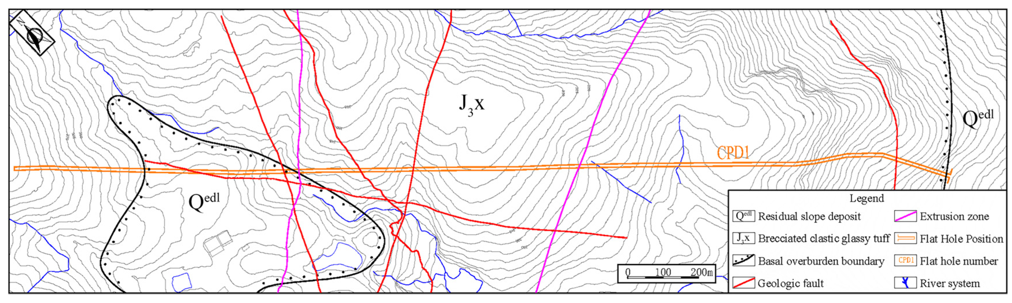
The Zhejiang Qingtian pumped storage power station is located in the middle of the mountainous area of South Zhejiang, belonging to the Donggong mountain range. The mountain ranges in this area mostly spread in the northeast direction, which belongs to the middle mountain–alpine landform. The outcrop beds in this area are relatively simple, mainly in the Upper Jurassic (J₃x). The quaternary overburden is sporadically developed and is dominated by alluvial deposits (Q₄^al+pl), residual slope deposits (Q₄^el+dl), and colluvial slope deposits (Q₄^col+dl), and it is mainly distributed in gully, slope, foot of slopes, and low-lying areas. Geotectonically, it belongs to the middle part of the Linhai–Wenzhou southeastern Fujian volcanic fracture and the arrhythmic depression belt (Ⅱ₂) of the South China Fold System (Ⅱ). The geological structure in this area is dominated by ruptures, and folds are not developed. The physical geological phenomena in the engineering area are mainly manifested as weathering and unloading of rock masses. The collapse mainly develops in the steep slope area of the bedrock, and the distribution range is small. The main surface runoff in the project area is Chengmen Keng gully and Jupu Yuan gully. The tributaries along the way are dendritic, and the water system is developed. Most gullies have seasonal flow, and the water quantity varies greatly with rainfall. The groundwater in the engineering area can be divided into bedrock fissure water and porous diving. Bedrock fissure water is endowed in bedrock fissures and fault fracture zones and is dominated by submerged types; the porous diving is distributed in the fourth system cover and fully weathered rock (soil) layer. The depth of burial varies directly by the atmospheric precipitation recharge, seepage along the cover or bedrock surface, or lateral recharge of bedrock fissure water.

The surrounding rock of CPD1 consists mainly of gravelly crystalline glassy tuff, greenish gray and light purplish red tuff and block structures, a gravel content of 5~10%, glassy debris mostly in the form of finely elongated angstroms, and quartz and potassium feldspar as the crystalline minerals (see Figure 1). Flat caves expose rock bodies that are mostly slightly weathered, with undeveloped faults. Joints are generally developed in the cave, dominated by medium–steep dips toward NW and NNW, mostly intersecting at a large angle to the axis of the cave. There is a water seepage phenomenon along the fault tectonic zone and the open fissure in the flat cave, where a local linear or a small water surge is formed.

3. Grouping of Joint Dominant Occurrence and Statistical Homogeneous Zone Segmentation

3.1. Joint Dominant Occurrence Grouping

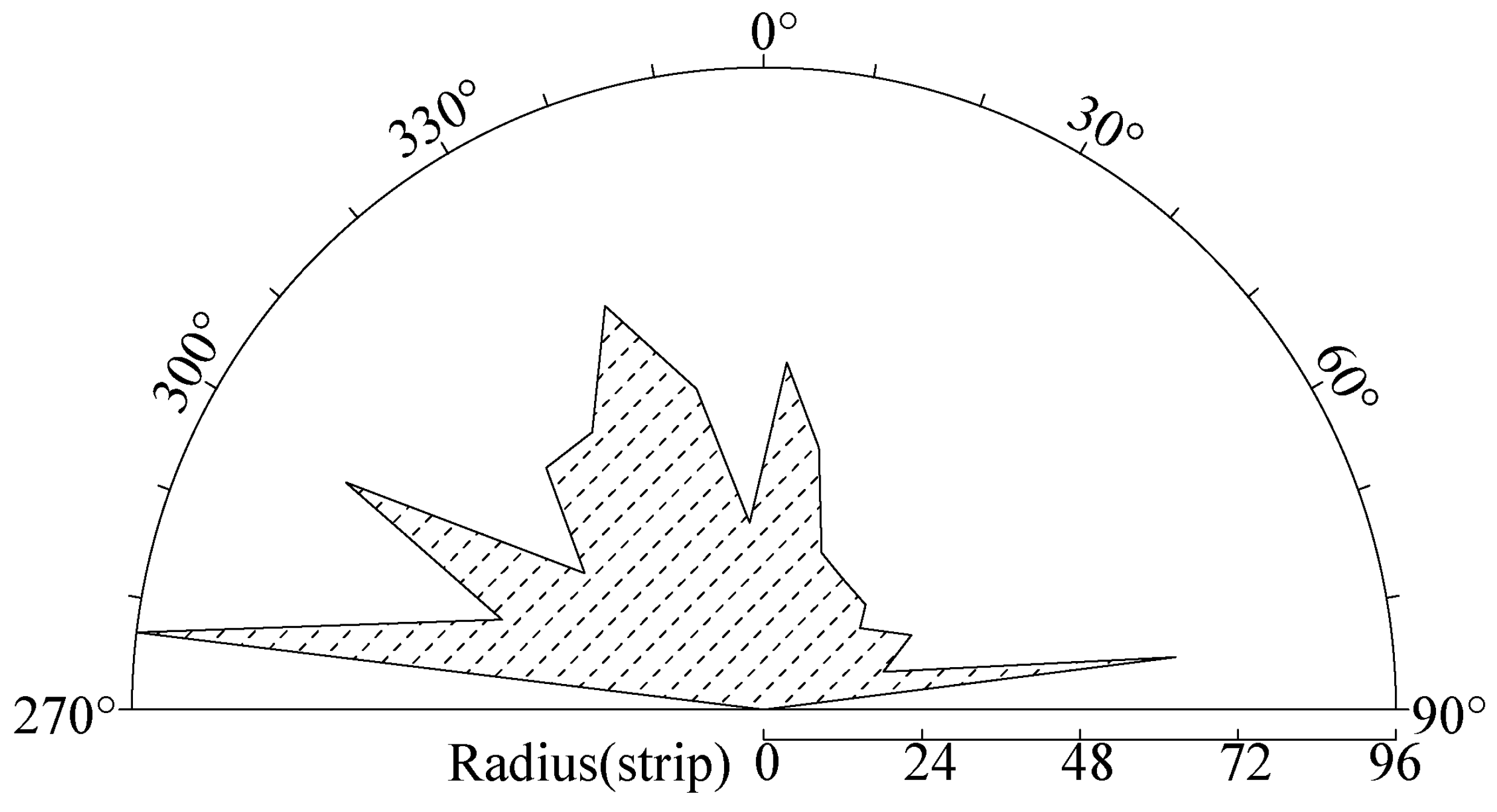
The long exploratory cave CPD1 is 800 m and the cave’s rock exposures are complete. On site, a measuring window with a length and width of 3m was used to carry out statistics on rock joints in a flat cave, and a total of 772 joints were measured. Researchers drew joint distribution maps based on on-site sketches (see Figure 2). The statistical data of 772 joints were regarded as Fischer distributions, and the joint rose diagram (see Figure 3) and the joint pole isodensity diagram (see Figure 4) were generated. On the basis of probabilistic statistics knowledge and Schmitt’s equal-area projection of the lower hemisphere, the optimal radius of the small sphere was determined through cyclic trial calculation, and the optimal grouping was determined by minimizing the objective function. Finally, the above joints were divided into five groups (see Figure 4 and

Table 1. Joint grouping parameters of CPD1 cave rock mass.

Group	Quantity/Strip	Dip Direction Range (°)	Dip Angle Range (°)
1	253	216~315	70~89
2	196	1~60	53~88
3	137	150~215	70~88
4	96	75~120	65~89
5	90	320~358	50~89

).

3.2. Statistical Homogeneous Zone Segmentation

In order to determine the boundaries of similar structural rock bodies, the areas with similar geomechanical properties are categorized into the same section, so that the rock bodies in each region have similar structural and mechanical characteristics. The principles of segmentation are as follows. (a) To meet the scale requirements of rock body classification, the appropriate structural classification scale is conducive to the evaluation of the quality of the rock body and the design of the rock body support. (b) To meet the number of samples for statistical analysis, the number of statistical samples of the joints in each segment has to be more than 100, and credible statistical results can be obtained [25].

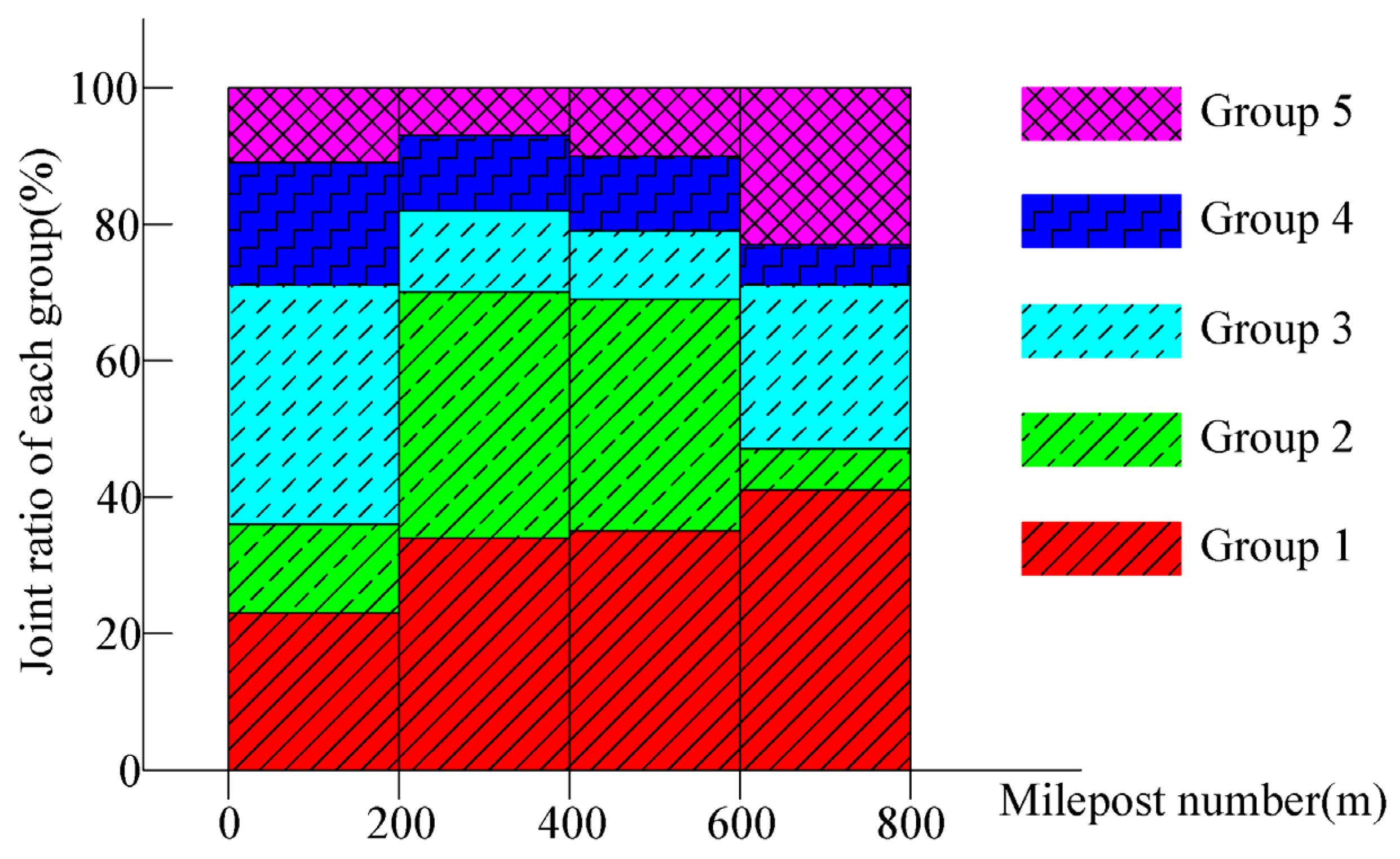
According to the above segmentation principle, using S.M. Miller’s rock structure zoning principle [26], the CPD1 flat cave was divided into four sections of 200 m each (see

Table 2. Segmentation and parameters of homogeneous zone in CPD1 cave rock mass.

Section	Starting Point (m)	Ending Point (m)	Number of Joints (Strip)	Average Density (Strip/m)
①	0	200	141	0.705
②	200	400	279	1.395
③	400	600	190	0.95
④	600	800	162	0.81

and Figure 5). It can be seen from Figure 5 that in Section ①, the joint composition of cave rock mass is relatively complex, the proportion is relatively average, and the average density of joint is relatively low. In Sections ② and ③, cave rock mass is dominated by the joints of group 1 and group 2, with an average proportion of 34.3% and 35.7%, respectively, as well as the highest average density of joints, at the 200~400 m segment. In Section ④, the cave rock mass is dominated by the joints of group 1, with an average proportion of 41.4%. Based on the above analysis, there are certain differences in the structural types of rock masses in each section due to the varying degrees of joint development. Therefore, it is necessary to conduct separate research on the rock masses of each section of the cave.

4. Probability Model of Joint Parameters

4.1. Probability Model of Joint Occurrence

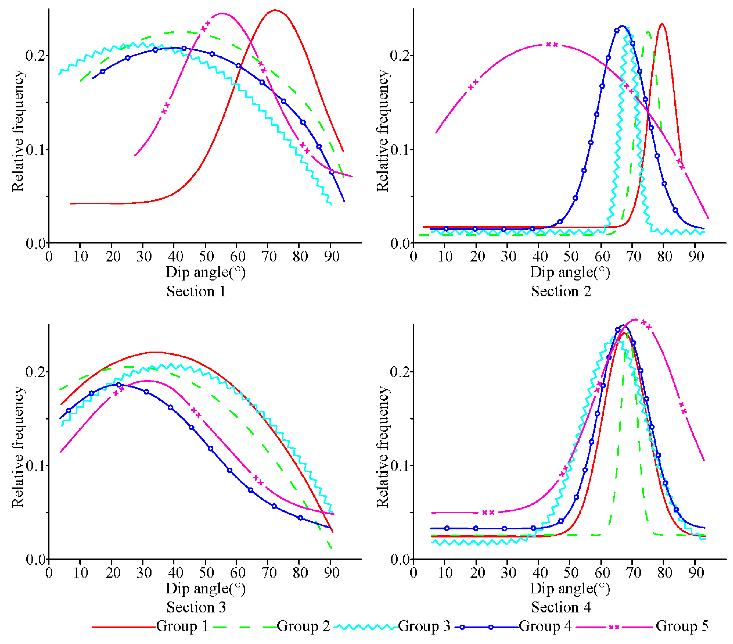
When the measuring window method is used for joint statistics, the occurrence relationship between the joint and the measuring window determines the probability of joint statistics. That is, sampling deviation exists in the statistical process. Therefore, it is necessary to correct the sampling deviation of the joint by using the method of weight coefficient. The probability model is studied based on the modified joint occurrence parameters. According to the results of the occurrence division of each joint dominant group in the study area, the occurrence frequency distribution of each dominant group was statistically analyzed, and the probability density curve of dominant occurrence was drawn (see Figure 6 and Figure 7).

The data analysis of Origin 2019b was used to fit a nonlinear curve to the frequency of joint yield distribution for each group of joints in each section to obtain its probability density curve. From the graph, a preliminary judgment is made that the dip direction and the dip angle may obey a normal or lognormal distribution. During curve fitting, the goodness of fit R2 was calculated, and the value of goodness of fit R2 was close to 1, indicating a good degree of fitting. In fitting the probability distribution of joint occurrence, the goodness of fit of the dip direction and dip angle of each segment ranged from 0.88 to 0.94. It was therefore considered that the fitting degree was good. Dip direction and dip angle obey the standard normal distribution in general. From this, the probabilistic model and its parameters were determined for the dip direction and dip of each group of joints in each section (see

Table 3. Calibration of the parameters of the probabilistic model of the modified joint geometry elements.

Section	Group	Dip Direction		Dip Angle		Diameter	Linear Density (Strip/m)	Volume Density (Strip/m3)
		Expectant (°)	Standard Deviation	Expectant (°)	Standard Deviation	Expectant (m)
①	1	251.3	6.51	52.8	4.32	3.65	0.42	0.46
	2	30.7	7.67	74.0	3.75	2.89	0.28	0.09
	3	189.8	3.93	60.0	4.45	2.67	0.62	0.12
	4	97.0	9.87	72.3	4.55	2.30	0.46	0.13
	5	351.3	1.09	64.9	2.09	4.96	0.28	0.16
②	1	260.4	3.07	73.6	7.83	1.97	0.76	0.28
	2	27.3	2.91	78.6	7.67	3.75	0.86	0.08
	3	186.3	2.19	73.0	7.15	1.49	0.38	0.25
	4	95.9	5.01	66.4	8.04	1.23	0.56	0.54
	5	348.7	7.01	63.6	8.61	4.88	0.44	0.02
③	1	257.6	5.10	74.2	6.59	2.19	0.86	0.26
	2	24.3	7.17	74.9	6.27	2.73	1.02	0.20
	3	195.0	4.97	63.3	5.67	1.50	0.36	0.23
	4	86.3	5.41	81.2	5.59	1.05	0.56	0.74
	5	340.7	8.77	70.6	7.73	4.90	0.26	0.15
④	1	274.6	6.82	71.5	5.83	2.89	0.86	0.15
	2	31.0	1.57	70.8	5.99	1.67	0.14	0.07
	3	179.3	5.53	77.6	5.94	2.34	0.40	0.10
	4	95.8	8.55	73.2	6.37	0.68	0.28	0.88
	5	346.1	5.64	59.9	6.23	3.67	0.46	0.05

).

4.2. Probability Model of Joint Diameter

The size of the joint can be expressed by the diameter of the disk, but in reality, because the diameter of the joint is difficult to measure directly, the joint diameter can be estimated indirectly by the length of the joint trace [27]. The measured window method was used for joint statistics, and the joints fell within the statistical window in three ways: contained, cut, and intersected [28]. During the statistical process, it was found that most of the medium–steeply dipping grown-up joints were developed in the study area, cut and jointed joints were more developed, and contained joints were very few. Joint trace length estimation methods include the point estimation method, the circular statistical window method, the H-H trace length estimation method, the generalized H-H trace length estimation method, and the Lastett trace length estimation method. According to the joint development characteristics and the relationship between the joint and the measuring window, as well as the comparison of the calculation results of various trace length estimation methods, the generalized H-H trace length estimation method has a better calculation accuracy, so the generalized H-H trace length estimation method is adopted [29,30] to calculate the joint trace length in the study area:

$$L=\frac{N_1+2N_0}{N}\frac{\left({\phi }_2-{\phi }_1\right)h}{\cos {\phi }_1-\cos {\phi }_2}+\frac{1}{N}{\sum }_{i=1}^{N_2}{X}_i$$

(1)

where $N$ is the total number of a certain group of joints in the statistical window; $N_0$ is the number of joints in the cutting relationship; $N_1$ is the number of joints in the connection relationship; $N_2$ is the number of joints containing the relation; $\phi$ is the angle between the trace line of the structural surface and the top or bottom edge of the window; and $X_i$ is the visible trace length of the node of the $i$th inclusion relation.

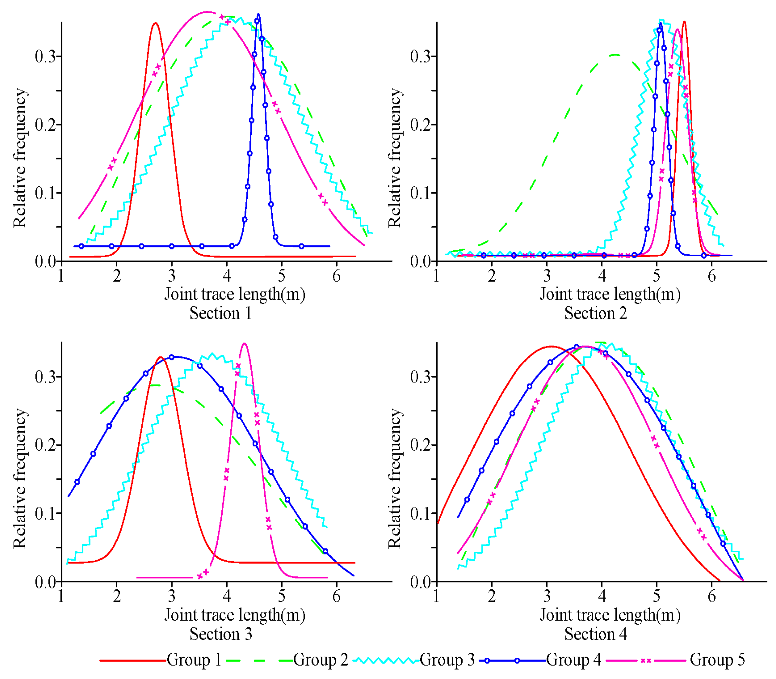
The relative frequency of each group of trace lengths in each segment was calculated using Formula (1), and the nonlinear curve was fitted to it (see Figure 8). The trace length of each group obeys the standard normal distribution, and the goodness of fit ranges from 0.87 to 0.93. The fitting result is accurate.

Jia and Pan studied and counted various trace length theoretical distribution functions [31,32]. When the trace length distribution function follows the standard normal distribution, the probability density function is

$$h\left(L\right)=\mu [1-{\int }_0^{L}f\left(L\right)dL]$$

(2)

for which:

$$f\left(L\right)=\frac{1}{\sqrt{2\pi \sigma }}{e}^{-\frac{{\left[L-\frac{1}{\mu }\right]}^2}{2{\sigma }^2}}$$

(3)

where $L$ is the trace length of the joint; $\mu$ is the center point density of the joint trace, $\mu$ = 1/$\overline{L}$; $\overline{L}$ is the average trace length of the joint; ${\sigma }^2$ is the variance of the overall distribution of joint trace length; and $f\left(L\right)$ is the trace length probability distribution function.

Assuming that joint diameter $D$ follows $f_D\left(D\right)$ distribution, then:

$$f_D\left(D\right)=\frac{\pi }{4}f\left(\frac{\pi }{4}D\right)$$

(4)

Then, the average joint diameter $\overline{D}$ can be expressed as follows:

$$\overline{D}={\int }_0^{\mathrm{\infty }}D{f}_D\left(D\right)dD=\pi {\int }_0^{\mathrm{\infty }}Df\left(\frac{\pi }{4}D\right)dD$$

(5)

According to the above analysis, the trace length probability density function of different groups of each homogeneous differentiation section is brought into Formula (5) to calculate the joint diameter and determine the probability model parameters of each group of joint diameters (see Table 3).

4.3. Estimation of Joint Density

The overall number of joints in the flat cave is determined by the joint volume density, which can be extrapolated from the joint line density. Joint line density ${\lambda }_d$ refers to the number of joints intersecting the measurement line per unit measurement line length. In general, the joint line density is obtained directly via the line measurement method when the joints are counted on site. The joint shape is assumed to be a thin disk, and the formula ${\lambda }_v$ is as follows [33]:

$${\lambda }_d=\pi {\lambda }_v{\int }_0^{\mathrm{\infty }}R{\int }_R^{\mathrm{\infty }}{f}_r\left(r\right)drdR$$

(6)

where $R$ is the distance from the intersection point between the measuring line and the disk to the outer edge of the joint; $f_r\left(r\right)$ is the probability distribution of the joint diameter.

The joint volume density is related to the joint line density and the average trace length. When the joint morphology conforms to the assumed thin disk, the approximate calculation can be obtained via the following:

$${\lambda }_v=\frac{2{\lambda }_d}{{\pi }^2{\overline{L}}^2}$$

(7)

where ${\lambda }_v$ is the joint volume density; ${\lambda }_d$ is the joint line density, which can be obtained through statistical calculation; and $\overline{L}$ is the average trace length of the joint.

$f_r\left(r\right)$ can substitute the probability distribution of joint trace length of different groups of each homogeneous section into Formula (4), and the volume density of each group of joints in each section can be calculated according to Formula (7). The results are shown in Table 3.

5. Classification of Rock Mass Structure Based on 3D Rock Block Index

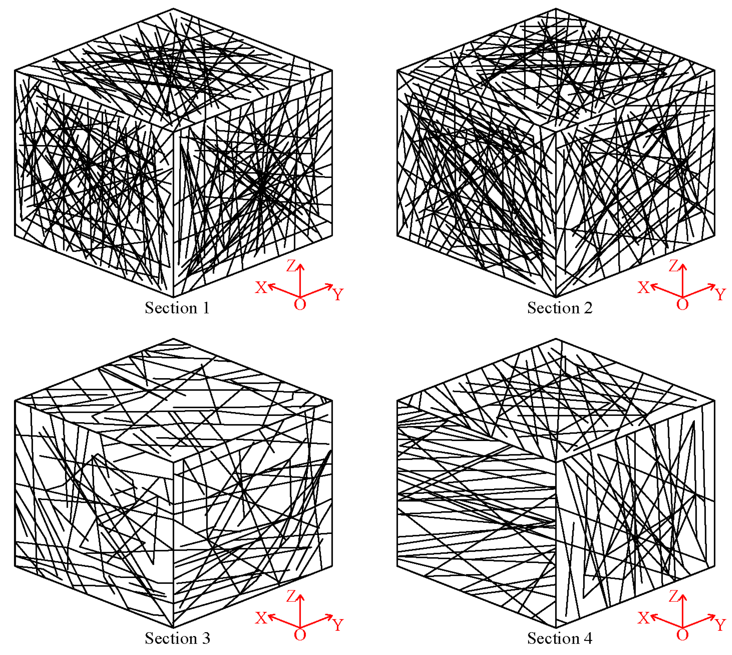
5.1. 3D Joint Network Simulation

Based on the probability model and parameters of geometric elements such as occurrence, diameter, and volume density of each group of joints, the Monte Carlo method was used to carry out a random simulation. According to the scope of the study area and the size of the measured joint, the size of the data generation area was determined to be 5 m × 5 m × 5 m, considering that the distribution of joints had edge effects and the size of the application area was included in the generation area. The size of the data application area was 3 m × 3 m × 3 m, determined by cutting into the data generation area. Adjust the orientation of the application area so that one side of it is consistent with the excavation direction of the flat cave, and use the 3D visualization technology to generate the 3D joint network model of the flat hole (see Figure 9).

The test methods of graphical comparison and data comparison were applied to carry out the validity test of the above 3D joint network model. Among them, the graphic comparison is realized by naked eye comparison, and the error is large. The indicators of data comparison include joint occurrence, diameter, etc. Generally, when the relative error is less than 20%, the model data are similar to the prototype data. Taking section ① as an example for detailed explanation, the 3D joint network model was cut, and the ideal cross-section was taken for graphical and data comparison with the measured flat cave joint distribution map, measured joint occurrence, and other data, respectively (see Figure 10 and Figure 11 and

Table 4. Data comparison accuracy analysis results.

Index	Group	Simulation Results	Relative Error (%)
		Expectant
Dip direction (°)	1	247.8	1.4
	2	28.1	8.4
	3	186.2	1.9
	4	92.5	4.6
	5	335.1	4.6
Dip angle (°)	1	49.5	6.3
	2	69.5	6.1
	3	55.6	7.3
	4	70.0	3.2
	5	61.5	5.2
Diameter (m)	1	3.7	16.7
	2	2.9	15.4
	3	2.8	10.2
	4	2.3	12.0
	5	5.0	11.4

).

A comparative analysis of the two-dimensional nodal trace distribution maps of the nodal network model is shown in Figure 10 and Figure 11. It is consistent with the actual distribution of joints sketched in the field in terms of profile exposure. As can be seen from Table 4, the relative error of each indicator of the 3D joint network model involved in the data comparison is less than 20%. The above two methods are used to test the ②, ③, and ④ sections, respectively, and the results are obtained within the permissible range. In summary, it is shown that the 3D joint network model has a good statistical similarity with the actual joint distribution, and the simulation results are relatively satisfactory and basically meet the requirements of accuracy.

5.2. Three-Dimensional Rock Block Index

The rock block index (RBI) is defined as the cumulative value of the product of the measured core lengths in flat caves or boreholes in terms of core acquisition rates of 3~10 cm, 10~30 cm, 30~50 cm, 50~100 cm, and greater than 100 cm as weights, multiplied by their respective corresponding coefficients [19]:

$$RBI=3\times C_{r3}+10\times C_{r10}+30\times C_{r30}+50\times C_{r50}+100\times C_{r100}$$

(8)

where $C_{r3}$, $C_{r10}$, $C_{r30}$, $C_{r50}$, and $C_{r100}$ are the core acquisition rates for cores 3–10 cm, 10–30 cm, 30–50 cm, 50–100 cm, and greater than 100 cm in length, expressed as percentages and considered as weights.

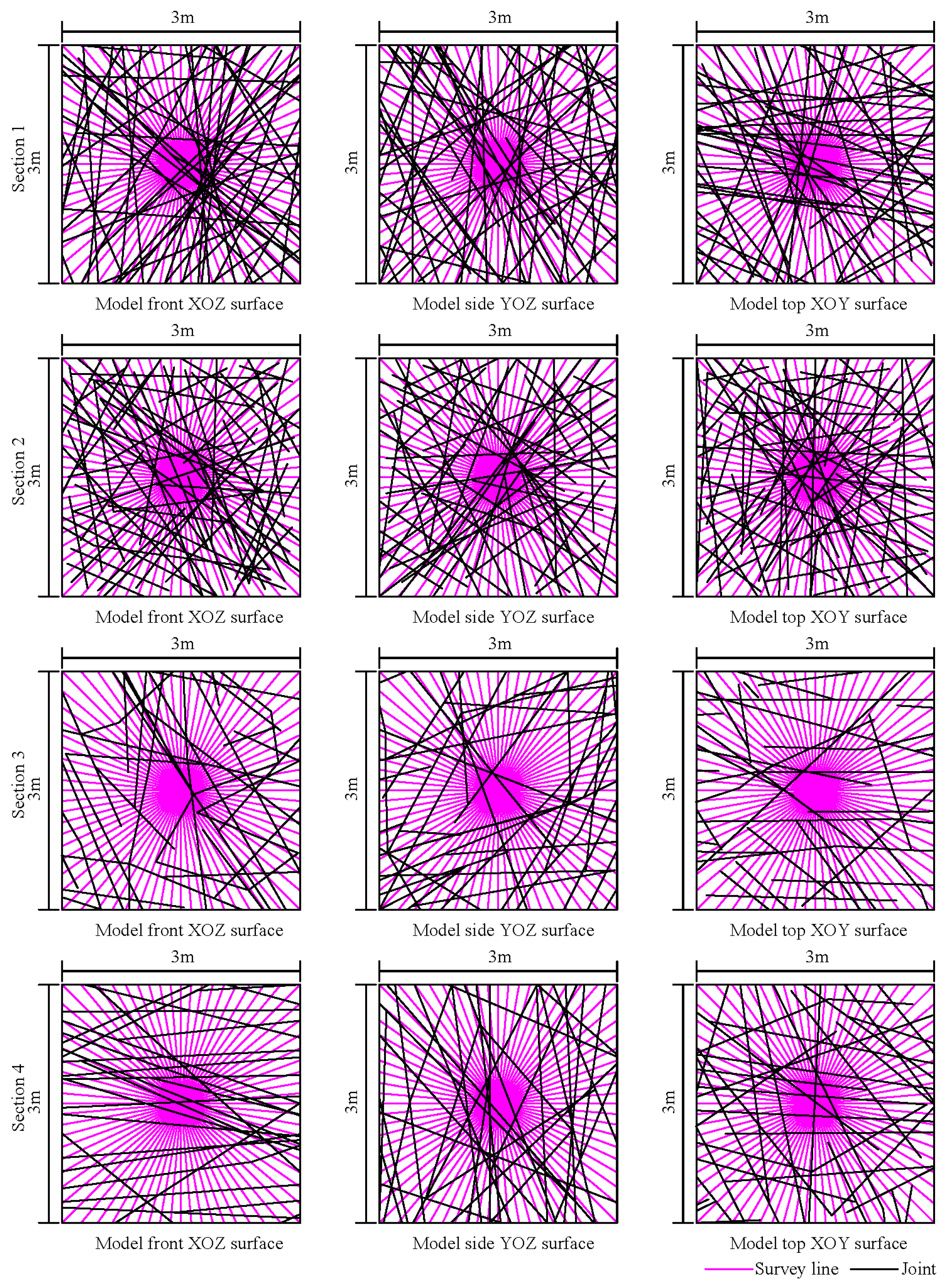
Because the excavation of the flat cave was carried out via blasting operations, it was not possible to directly obtain the complete core take rate, so the above 3D joint network model was used instead and virtual survey lines were arranged in different sidewalls to represent the boreholes. According to the intersection and tangency between the joint and survey lines, the spacing between the joint and survey lines was measured, and the rock block indexes of the different boreholes were obtained through the calculation of Formula (8). The RBI value of rock block index obtained using one borehole could only determine the structural characteristics of the exposed wall in the direction of the borehole or a certain excavation in the flat hole, and it was not possible to evaluate the three-dimensional structural characteristics of the rock mass. Therefore, the concept of a 3D rock block index was proposed. It is the expected value of borehole RBI in different orthogonal planes.

In the model, the XOZ surface, which is parallel to the excavation surface of the flat cave, is defined as the front surface of the model; the vertical YOZ surface, which is perpendicular to the excavation surface, is defined as the side surface of the model; and the XOY surface, which is perpendicular to both the XOZ surface and the YOZ surface, is defined as the top surface of the model. The above three orthogonal planes were selected for the study of rock structure characteristics, and in each orthogonal plane, 36 virtual survey lines were arranged at equal angles centered on the form center and at 5° intervals, for a total of 108 survey lines (see Figure 12). After counting the RBI values corresponding to the 36 virtual survey lines on different orthogonal planes, the RBI values on different orthogonal planes are obtained (see

Table 5. Rock block index and rock mass structure classification results of each.

Section		RBI Scope	RBI Mean Value	3D Rock Block Index	Rock Mass Structure Type
①	Model front surface	39.12~42.19	40.66	41.18	Blocky structure
	Model side surface	35.81~41.32	38.20
	Model top surface	41.10~48.24	44.69
②	Model front surface	35.51~45.25	39.14	43.19	Blocky structure
	Model side surface	40.19~48.98	44.62
	Model top surface	39.20~48.61	45.81
③	Model front surface	55.35~59.42	58.41	56.38	Overall structure
	Model side surface	51.60~58.12	54.81
	Model top surface	52.10~58.84	55.90
④	Model front surface	57.32~64.98	61.80	61.87	Overall structure
	Model side surface	57.88~63.25	59.93
	Model top surface	60.88~66.99	63.88

). It can be seen that the distribution of RBI values is different for each orthogonal plane.

5.3. Classification of Rock Mass Structure

Rock mass quality classification is an indispensable link in rock mass engineering. With regard to the research performed on rock mass quality classification, domestic and foreign experts as well as scholars have conducted a substantial amount of work. Now, it has formed a relatively perfect system. Since the 1970s, different rock mass quality classification methods, such as RMR, SMR, RMS classification, and E. Hoek’s GSI classification, have been proposed successively for the classification system of rock mass quality in hydropower engineering [34,35,36,37]. The classification of rock mass structure types is the basis of rock mass quality classification evaluation. It can comprehensively reflect geological characteristics, structural plane properties, rock strength, rock deformation characteristics, and other semi-quantitative indexes. Evert Hoek [38] conducted a detailed analysis of the mechanical properties of rock mass through experiments and classified the rock mass into four types of structures: loose structure, cataclastic structure, secondary block structure, and blocky structure. According to the classification standard of rock mass structure in the national standard “Code for Geological Investigation of Water Conservancy and Hydropower Engineering” (GB50287-99) and the definition of RBI, Hu proposed the classification standard of rock mass structure based on RBI [19,39].

According to the RBI index, rock structures can be divided into six types (see

Table 6. RBI index classification and qualitative description of rock mass structure type.

Classification	RBI Value	Structural Characteristics of Rock Mass	Rock Mass Structure Type
Ⅰ	50~100	The rock mass is extremely complete, and the structural planes are not developed	Overall structure
Ⅱ	30~50	The rock mass is complete	Blocky structure
Ⅲ	10~30	The rock mass is relatively complete	Secondary block structure
Ⅳ	3~10	The rock mass is relatively fragmented or with poor integrity	Mosaic structure
Ⅴ	1~3	The rock mass is fragmented and the structural planes are well-developed	Cataclastic texture
Ⅵ	<1	The rock mass is extremely fragmented in a loose and massive state	Loose structure

).

The 3D rock block index is used as a quantitative evaluation index to determine the rock mass structure of the flat cave, and based on the classification criteria of the RBI index in Table 6, the rock mass structure of each statistically homogeneous section of the long exploratory cave CPD1 is classified. The classification results for rock mass structure are shown in Table 5. In order to verify the reasonableness of the above rock mass structure classification results, a flat cave seismic wave physical exploration test was carried out on the long exploration cave CPD1. The measured seismic wave depth of the flat cave is 0~800 m. The surveying line is arranged on the left wall of the flat cave, 1 m high from the bottom of the cave. Based on the first clear P-wave record and the continuous S-wave record of the same phase axis, $t_P\left(\mathrm{x}\right)$ and $t_s\left(\mathrm{x}\right)$ of the initial arrival phase of the P-wave and S-wave at each detection point are obtained from the original seismic record. Then, the ${\theta }_P\left(\mathrm{x}\right)$ and ${\theta }_s\left(\mathrm{x}\right)$ curves are calculated. Then they are used to calculate the longitudinal and transverse wave velocities in the rock, as follows:

$$v_P=2\frac{\Delta x}{\Delta {\theta }_P}$$

(9)

$$v_s=2\frac{\Delta x}{\Delta {\theta }_s}$$

(10)

where $v_P$ is the longitudinal wave velocity of rock mass; $v_s$ is the transverse wave velocity of the rock mass; $\Delta x$ is the distance difference on the time distance curve; $\Delta {\theta }_P$ is the time difference on the ${\theta }_P\left(\mathrm{x}\right)$ curve; $\Delta {\theta }_s$ is the time difference on the ${\theta }_s\left(\mathrm{x}\right)$ curve; and the unit for each of the above parameters is m/s.

According to the measured longitudinal and transverse wave velocities of the flat cave rock mass, the integrity coefficient of the rock mass is calculated via Formula (11). The seismic wave test results are shown in

Table 7. CPD1 seismic wave test comprehensive results table.

Starting Point (m)	Ending Point (m)	Range Value of KV	Average Value of KV	Integrity Evaluation
0	200	0.53~0.75	0.71	Relatively complete
200	400	0.56~0.72	0.70	Relatively complete
400	600	0.76~0.84	0.78	Complete
600	800	0.78~0.87	0.83	Complete

.

$$k_v=\frac{v_P}{v_{Pr}}$$

(11)

where $v_P$ is the longitudinal wave velocity of rock mass; $v_{Pr}$ is the acoustic longitudinal velocity of the intact and fresh rock mass. According to the previous and current test results, the $v_{Pr}$ value of fresh rock mass is 6000 m/s.

The seismic wave test of a flat cave is based on the rock integrity coefficient K_V to classify the rock integrity. Based on the rock block index (RBI) and integrity coefficient K_V for the rock structure and integrity evaluation criteria, the qualitative description of the rock structure via the two methods is compared to obtain the correspondence between the two. According to Table 5, the classification results of rock mass structure based on the 3D rock block index are consistent with the field test results. Therefore, it is reasonable and feasible to use the 3D rock block index obtained from the joint network model as a quantitative evaluation index to determine the structural type of rock mass in flat caves.

6. Discussion

The 3D joint network simulation based on statistics and probability, which are in turn based on the statistical laws of various geometric elements of joints, can achieve the visualization of the rock mass structure. On this basis, the 3D rock block index is applied to carry out the structural classification of flat cave rock mass, which overcomes many limitations of traditional rock mass structure classification:

(1)

Overcoming the limitation of having a single disaggregated indicator. The traditional rock structure classification is related to the rock quality index (RQD) except for the water conservancy and hydropower perimeter rock engineering geology classification method, which does not use the rock quality index (RQD). The classification index is single, and the RQD itself has shortcomings. For example, for a rock mass with RQD = 90%, the block composition can be any size greater than 10 cm. However, the integrity of rock mass varies greatly with different block compositions. This suggests that the RBI values more accurately reflect the structural characteristics of the rock mass than the RQD.

(2)

Overcoming the limitation of dimension. From the definition, the rock block index (RBI) is a one-dimensional index, while the rock mass is a three-dimensional space. The same rock mass structure can be calculated to have different RBI values when the measurement statistics of the boreholes are taken along different directions, which indicate that the distribution of the rock mass joints tends to have obvious anisotropy, and the use of single-direction measurements to categorize the rock mass structure is inaccurate. Therefore, expanding one-dimensional indicators into three-dimensional ones can provide a more realistic response to the rock structure.

It is worth noting that field site counts of core lengths in flat caves or boreholes are based on weathering, unloading, or structural-type segmentation of the rock mass. In terms of distribution probability, the range of RBI values in different directions of a certain rock mass with certain weathering type or structural type is also determined, and the corresponding relationship is very close. In addition, the 3D joint network simulation is a non-physical simulation, which is only the same as the actual rock mass at the level of statistical probability, but not in a specific position, that is, the “simulation” of the 3D joint simulation. Therefore, extensive and detailed statistics on the original statistical data of joints can effectively improve the precision of 3D joint network simulation, and the obtained 3D rock block index can more accurately reflect the actual rock mass structural characteristics.

7. Conclusions

(1)

Taking the rock mass of the long exploratory cave CPD1 in the water transmission system of the Qingtian pumped storage power station in Zhejiang province as the research object, the rock mass of the flat cave is statistically homogeneous, and the probability model of joint parameters in each homogeneous zone is obtained.

(2)

According to the probabilistic model of joint parameters, the Monte Carlo method was used to develop stochastic simulations of joints, and the 3D network model of joints in the rock mass of a flat cave in each segment was established. Through the comparison of graphs and data, it is concluded that the 3D joint network simulation based on statistics and probability can realize the visualization of rock mass structure, effectively improve the precision of the 3D joint network simulation, and more accurately reflect the structural characteristics of actual rock mass.

(3)

Based on the 3D joint network model, virtual survey lines are arranged on the front, side, and top surfaces of the model to represent the borehole, and the RBI values of 108 virtual survey lines on the three orthogonal planes are counted. Using the concept of 3D rock block index, the fine classification of the flat cave rock mass structure is conducted. The results of the structural classification of flat cave rock mass based on the 3D rock block index show that the rock mass structure of the long-tunnel CPD1 is classified as that which is from overall structure to blocky structure, corresponding to the integrity of rock mass being complete to relatively complete. The classification results are consistent with the evaluation results of horizontal tunnel seismic wave geophysical exploration.

(4)

Compared with traditional rock mass classification methods and classification indexes, the 3D rock block index can more accurately reflect the structural characteristics of rock mass. It can be used as a quantitative index to directly reflect the anisotropy of rock mass structure in three-dimensional space. Therefore, it is reasonable and feasible to use the 3D rock mass index as a quantitative evaluation index to analyze the type of rock structure, and it is helpful and meaningful in the classification of underground engineering rock structures.

References

- Sun, G.Z. Theory and Practice of Geological Engineering; Seismic Press: Beijing, China, 1996; pp. 56–58. [Google Scholar]
- Sun, G.Z. Basis of Engineering Geo Machanics of Rock Mass; Sciences Press: Beijing, China, 1983; pp. 134–138. [Google Scholar]
- Sun, G.Z. Mechanics of Rock Structures; Science Press: Beijing, China, 1988; pp. 75–77. [Google Scholar]
- Tao, Z.Y. Theory and Practice of Rock Mechanics; Water Conservancy Press: Beijing, China, 1981; pp. 137–138. [Google Scholar]
- Sheng, D.; Yu, J.; Tan, F. Rock mass quality classification based on deep learning: A feasibility study for stacked autoencoders. J. Rock Mech. Geotech. Eng. 2023, 15, 1749–1758. [Google Scholar] [CrossRef]
- Han, A.G.; Nie, D.E.; Sun, G.P. Determination of spacing of structural plane in rock mass structure research. Chin. J. Rock Mech. Eng. 2003, z2, 3. [Google Scholar]
- Ding, W.X.; Yao, Z.; Jiang, Z. Study on methods of how to select reasonably elastic wave velocity parameters of engineering rock mass. Rock Soil Mech. 2004, 25, 1353–1356. [Google Scholar]
- Yin, M.L.; Zhang, J.X.; Jiang, Y.S. Study of correction of the structural plane category based on the rock mass integrity coefficient characterized by the volumetric joint count. Rock Soil Mech. 2021, 42, 1133–1140. [Google Scholar]
- Du, S.G.; Xu, S.F.; Yang, S.F. Application of rock quality designation (RQD) to engineering classification of rocks. J. Eng. Geol. 2000, 8, 6. [Google Scholar]
- Palmstrom, A. The volumetric joint count—A useful and simple measure of the degree of rock mass jointing. In Proceedings of the 4th International Congress of International Association of Engineering Geology, New Delhi, India, 11–15 June 1982; pp. 221–228. [Google Scholar]
- Ruan, Y.; Chen, J.; Fan, Z. Application of K-PSO Clustering Algorithm and Game Theory in Rock Mass Quality Evaluation of Maji Hydropower Station. Appl. Sci. 2023, 13, 8467. [Google Scholar] [CrossRef]
- Palmstrom, A. Application of the volumetric joint count as a measure of rock mass jointing. In Proceedings of the International Symposium on Fundamentals of Rock Joints, Bjorkliden, Sweden, 15–20 September 1985; pp. 103–110. [Google Scholar]
- Liu, T.; Jiang, A.; Zhang, Z. Estimation of the Lengths of Intact Rock Core Pieces and the Corresponding RQD considering the Influence of Joint Roughness. KSCE J. Civ. Eng. 2023, 27, 2689–2703. [Google Scholar] [CrossRef]
- Jiang, Y.F.; Wang, S. Application of Rock Block Index in Classification of Wallrock in Vertical Shaft. Min. Eng. 2023, 14, 4. [Google Scholar]
- Wang, X.G. Study of determination methods of rock mass mechanical parameters II: Numerical simulation test. J. Hydraul. Eng. 2023, 54, 129–138. [Google Scholar]
- Zhao, X.; Zhu, Q.; Westman, E. Research on failure mechanism and support technology of fractured rock mass in an undersea gold mine. Geomat. Nat. Hazards Risk 2023, 14, 2221776. [Google Scholar] [CrossRef]
- Hasan, M.; Shang, Y.; Yi, X. Determination of rock mass integrity coefficient using a non-invasive geophysical approach. J. Rock Mech. Geotech. Eng. 2023, 15, 1426–1440. [Google Scholar] [CrossRef]
- Yusoff, I.N.; Ismail, M.A.M.; Tobe, H. Quantitative granitic weathering assessment for rock mass classification optimization of tunnel face using image analysis technique. Ain Shams Eng. J. 2023, 14, 101814. [Google Scholar] [CrossRef]
- Hu, X.W.; Zhong, P.L.; Ren, Z.G. Rock-mass block index and its engineering practice significance. J. Hydraul. Eng. 2002, 33, 80–83. [Google Scholar]
- Zhang, S.S. The characteristics of rock mass block at dam foundation. J. Eng. Geol. 2001, 9, 353–356. [Google Scholar]
- Zhu, J.Y.; Chen, Q.S.; Tan, J.S. Cluster analysis for joint data of three-dimensional rock mass using DifFUZZY method. J. Eng. Geol. 2023, 31, 1689–1695. [Google Scholar]
- Huang, R.Q.; Huo, J.J. Quantitative analysis of rock mass block index for dam foundation of Jinping Ⅰ hydropower station. Chin. J. Rock Mech. Eng. 2011, 30, 449–453. [Google Scholar]
- Ni, W.D.; Shan, Z.G.; Liu, X. Classification of rock mass structure of dam foundation based on 3D joint network simulation. Rock Soil Mech. 2018, 39, 287–296. [Google Scholar]
- Wang, M.F. 3D joint rock mass network modeling application using python. Soil Eng. Found. 2023, 37, 410. [Google Scholar]
- Ruan, Y.K.; Chen, J.P.; Li, Y.Y. Identification of homogeneous structural domains of jointed rock masses based on joint occurrence and trace length. Rock Soil Mech. 2016, 37, 5. [Google Scholar]
- Chen, J.P.; Wang, Q.; Xiao, S.F. Evaluation of statistical homogeneity of rock mass structure. J. Geol. Hazards Environ. Preserv. 1996, 01, 19–24. [Google Scholar]
- Wang, G.B.; Yang, C.H.; Bao, H.T. Mean trace length estimation of rock mass joint. Chin. J. Rock Mech. Eng. 2006, 25, 2589–2592. [Google Scholar]
- Kulatilake, P.H.S.W.; Wu, T.H. The density of discontinuity traces in sampling windows. Int. J. Rock Mech. Min. Sci. Geomech. Abstr. 1984, 21, 345–347. [Google Scholar] [CrossRef]
- Shen, Y.J.; Xu, G.L.; Dong, J.X. Relationship between mean trace length of joints and location of sampling window. Chin. J. Rock Mech. Eng. 2001, 30, 7. [Google Scholar]
- Huang, G.M.; Huang, R.Q. Estimating discontinuity trace length based on the intersection condition. Geol. Sci. Technol. Inf. 1999, 18, 3. [Google Scholar]
- Pan, B.T.; Jing, L.R. Computer simulation methods and applications of statistical models of rock mass structure. New Prog. Rock Mech. 1989, 1, 26. [Google Scholar]
- Jia, H.B.; Tang, H.M.; Liu, Y.R. Rock structural surface three-dimensional network simulation theory and its engineering application. Sci. Press 2008, 7, 64–69. [Google Scholar]
- Sen, Z.; Kazi, A. Discontinuity spacing and RQD estimates from finite length scanlines. Int. J. Rock Mech. Min. Sci. Geomech. Abstr. 1984, 21, 203–212. [Google Scholar] [CrossRef]
- Bieniawski, Z.T. Engineering classification of rock masses. Civ. Eng. S. Afr. 1973, 15, 335–344. [Google Scholar]
- Bieniawski, Z.T. Engineering Rock Mass Classifications. Petroleum 1989, 251, 357–365. [Google Scholar]
- Barton, N.; Lien, R.; Lunde, J. Engineering classification of rock masses for the design of tunnel support. Rock Mech Rock Eng. 1974, 6, 189–239. [Google Scholar] [CrossRef]
- Hoek, E.; Marinos, P.; Benissi, M. Applicability of the geological strength index (GSI) classification for very weak and sheared rock masses. The case of the Athens Schist Formation. Bull. Eng. Geol. Environ. 1998, 57, 151–160. [Google Scholar] [CrossRef]
- Hoek, E.; Marinos, P. A brief history of the development of the Hoek-Brown failure criterion. Soils Rocks 2007, 2, 1–13. [Google Scholar] [CrossRef]
- Ministry of Water Resources of the People’s Republic of China. Code for Geological Investigation of Water Conservancy and Hydropower Engineering (GB 50287-99); China Planning Press: Beijing, China, 1999.