Vehicle Trajectory Reconstruction Using Lagrange-Interpolation-Based Framework

Featured Application

This research contributes to the development of a technological method to obtain highly accurate vehicle trajectory data. The reconstructed trajectory data play a key role in traffic state prediction, traffic management and the decision making of autonomous vehicles and robots.

Abstract

Vehicle trajectory usually suffers from a large number of outliers and observation noises. This paper proposes a novel framework for reconstructing vehicle trajectories. The framework integrates the wavelet transform, Lagrange interpolation and Kalman filtering. The wavelet transform based on waveform decomposition in the time and frequency domain is used to identify the abnormal frequency of a trajectory. Lagrange interpolation is used to estimate the value of data points after outliers are removed. This framework improves computation efficiency in data segmentation. The Kalman filter uses normal and predicted data to obtain reasonable results, and the algorithm makes an optimal estimation that has a better denoising effect. The proposed framework is compared with a baseline framework on the trajectory data in the NGSIM dataset. The experimental results showed that the proposed framework can achieve a 45.76% lower root mean square error, 26.43% higher signal-to-noise ratio and 25.58% higher Pearson correlation coefficient.

1. Introduction

Outliers and observation noises of vehicle trajectory data deteriorate the value of the data in traffic state prediction and traffic management. Kovvali et al. pointed out that vehicle trajectory data could be used to construct the driving behavior model, such as car following, lane changing, cooperative driving, distance control and safe driving, and proposed a data transcription and extraction method from video data to vehicle trajectories [1]. Xie et al. proposed a non-parameter clustering Dirichlet process Gaussian mixture model (DPGMM) to extract vehicle trajectories from 70-h traffic video data at two intersections in Brooklyn and used hidden Markov models (HMMs) to recognize the rear-end conflict risk for adjacent vehicles [2]. Taylor et al. researched driver heterogeneity behavior and situation-dependent behavior in car-following scenes using large vehicle trajectory datasets and proposed a dynamic time-warping algorithm with a time parameter to calibrate the microscopic simulation model [3]. Chen et al. used heterogeneous traffic data to estimate the state of spatial-temporal traffic and capture traffic congestion [4]. Li et al. studied the cooperative perception framework of the vehicle microtraffic state based on freeway and arterial vehicle trajectory datasets [5]. Tsanakas et al. used a microemission model to solve the problem of insufficient trajectory data [6]. Rempe et al. proposed a deep convolutional neural network for the accurate estimation of space–time traffic speeds [7]. However, the vehicle trajectory data collected suffered from outliers and observation noises by the communication signal occlusion, severe weather environment and so on. Outliers are defined as data points that are significantly larger or smaller than the neighbor points. Lu et al. identified obvious trajectory outliers and observation noises in the Next Generation Simulation (NGSIM) trajectory dataset [8]. Punzo et al. used jerk analysis, consistency analysis and spectral analysis to assess the data accuracy of vehicle trajectory data, and the results of error statistics indicated that trajectory outliers and observation noises are common in many datasets, such as NGSIM [9]. Coifman et al. took the I-80 data to illustrate that there were many errors such as large acceleration and bumper position marking errors [10].

Identifying and correcting outliers of vehicle trajectory data is one of the topics. Thiemann et al. took the vehicle dynamic performance (such as maximum speed, acceleration time) as the judgment standard of abnormal speed and acceleration and used the moving symmetric index average method to repair outliers [11]. Ge et al. detected outliers based on outlying scores. An outlying score of a vehicle trajectory is calculated as the similarity between the direction vector of a trajectory and those of other trajectories [12]. Punzo et al. added a jerk and frequency spectrum to the threshold discrimination method based on the vehicle dynamic performance threshold [13]. Wang et al. proposed an expectation maximization (EM) algorithm to re-estimate the outliers [14]. Suvin et al. identified and deleted outliers by resampling missing data [15]. Zhou et al. used a time-varying completion method to estimate trajectory data [16]. Hu et al. used data quality evaluation to remove outliers in the Waymo Open Dataset (WOD) [17]. Many machine learning methods, such as the convolutional neural network (CNN), support vector machine (SVM) and so on, have been applied to predict trajectory data [18]. Chen et al. calculated the similarity between original trajectories and trajectories of a dataset by attention-based learning [19]. Belhadi et al. developed a clustering algorithm to cluster the potential outliers and a KNN algorithm to identify outliers from the cluster [20]. The methods deal with various types of outliers but require many calibrated parameters. Thomas et al. illustrated the simple structure of the Lagrange interpolation algorithm [21]. Liu et al. used trajectory historical information and network topology geometry information to construct a weighting-based map matching method to detect notable location errors and proposed an interpolation method with path determination and trajectory interpolation to solve the low sampling rate of vehicle trajectory data by GPS devices [22]. Wan et al. proposed a stacked autoencoder for detecting outliers of monitoring data. Based on the difference between the input and the output of the trained stacked autoencoder, the Grubbs criterion and the PauTa criterion are used to evaluate whether data points are outliers [23]. Peralta et al. proposed unsupervised deep neural network models based on stacked autoencoders to detect the outliers among position, speed and angular position [24]. Zhao et al. proposed a three-step vehicle trajectory reconstruction method with the wavelet transform, Gaussian kernel and Savitzky–Golay filter to reconstruct the trajectory data from 15 intersections. The framework used Gaussian-kernel-based locally weighted linear regression to interpolate the data after outliers were removed [25].

Observation noise removal has also received some research attention. Montanino et al. analyzed the reason for the observation noise and used a low pass filter to reduce the observation noise [26]. Thiemann et al. proposed a smoothing algorithm to denoise the data of the beginning segment and the ending segment of a vehicle trajectory [11]. Wang et al. used the Kalman filter to reduce the observation noise of vehicle trajectory data [27]. Frad et al. used the wavelet filter method to filter the observation noise of vehicle trajectory data [28]. Durrani et al. used a symmetric index moving average filter method to denoise in the NGSIM (US-101) dataset [29]. Chen et al. combined empirical mode decomposition (EMD), ensemble empirical mode decomposition (EEMD) and the wavelet transform to achieve noise suppression [30]. Hu et al. used the wavelet transform to denoise trajectory data [17]. It is known that the denoise and smoothing methods of trajectory data mainly include the moving average filter, Kalman filter and symmetric exponential average filter. Each denoising method has its advantages, but its parameters remain unchanged. Nithin et al. proposed a multiple-model filtering adaptive method to infer the observation noise and predict vehicle trajectories. The method integrated maximum-likelihood multiple-model filtering and the unscented Kalman filter (UKF). The adaptive UKF had been pretrained in the constant velocity model, constant turn rate model, constant acceleration model and constant turn rate and acceleration model [31]. Mahajan et al. used smoothing filters and extreme gradient boosting with adaptive regularization to reduce the observation noise between speed and acceleration. The method had better robustness in processing raw data from an unmanned aerial system compared with manual thresholds [32]. Abbas et al. proposed a multimodel-based extended Kalman filter (EKF) to reduce the vehicle location noise using the vehicle trajectory. The EKF used the velocity, position and distance of the vehicle to construct a state vector matrix and used probability calculation to obtain the predicted results [33]. Zhang et al. used a Kalman filter to reduce the noise of prediction uncertainty while predicting real-time cooperative vehicle trajectory with the kinematic and data-driven models [34]. Zhao et al. proposed a multi-objective optimization control method based on expanded state observers in order to keep the accuracy and stability, which are disturbed by a variety of factors in curved roads [35].

Built on the state of the art, the innovations of this study are summarized as follows: (1) A Lagrange-interpolation-based framework for vehicle trajectory reconstruction is proposed, which integrates the discrete continuous wavelet transform, Lagrange interpolation and the Kalman filter, which can obtain a smooth trajectory. (2) Two kinds of Lagrange interpolation polynomials are developed for reconstructing outliers between speed and acceleration in vehicle trajectory data, which improve computation efficiency.

The remainder of this study is organized as follows. Section 2 describes the problems of vehicle trajectory data that the paper is dealing with. Section 3 describes the methodology of the proposed vehicle reconstruction framework in the paper. Section 4 shows the processing reconstruction results of the framework by experiments. Section 5 discusses the reconstruction results between the proposed method and the baseline method. Section 6 concludes this work and recommends further research directions.

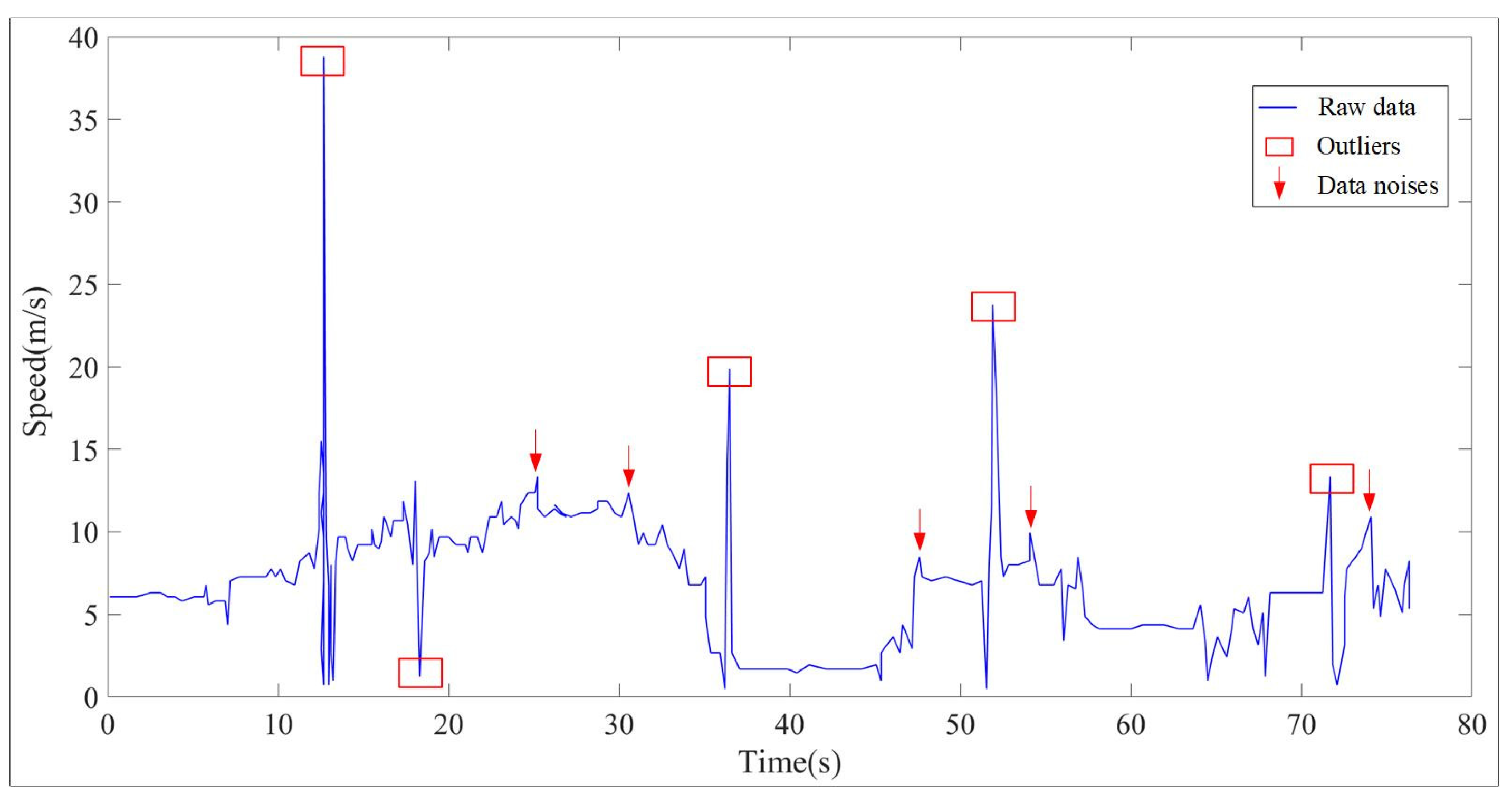
2. Problem Statement

Vehicle trajectory data are very important to analyze the microscopic phenomena in transportation systems. GPS devices have usually been used to collect trajectory data in the last decades, but vehicle location sensors can generate a large amount of outlier and observation noise due to a relatively low sampling rate and location error [22,24,31,36]. With the development of multimedia equipment, many transportation researchers have used high-resolution images to extract vehicle trajectory data, and the high-resolution images are from videos and cameras, which are installed on an unmanned aerial vehicle, a moving car or transportation infrastructures. But the immature computer vision extraction techniques in complex traffic environments (e.g., vehicles are obscured by buildings or bridges in some images) cause some unexpected data in extracted vehicle trajectory data [1,2,32].

The Next Generation Simulation (NGSIM) program uses videos and cameras to collect high-quality traffic datasets including vehicle trajectory data. It is a classic and publicly available dataset to support research on microscopic traffic state estimation and driving behavior. The paper uses the NGSIM dataset to test the proposed framework of vehicle trajectory reconstruction. According to previous studies [9,13,26,37], outliers and observation noise are common in trajectory data in the NGSIM dataset. The original data in NGSIM have recorded 25 types of information, such as vehicle ID, global time, velocity, acceleration and so on. Figure 1 presents the outliers and observation noises of the trajectory data of vehicle 1882 in the I-80 data subset. The speed is the longitudinal instantaneous speed obtained from the first derivative of the longitudinal position data.

Figure 1 shows that the original trajectory data generally have outliers and noises. The data points indicated by arrows are not much different from neighbor data, but the change in speed has exceeded the limit of vehicle dynamic performance and range of the body tolerance limit (−8 m/s², 5 m/s²). These rapidly changing data are considered as detection errors. The data points indicated by the rectangular are significantly different from neighboring data. The values do not conform to the rule of vehicle operation. The data from frames 518 to 522 are extracted to illustrate this problem in

Table 1. Outliers between frames 518 to 522.

Sequence Number	518	519	520	521	522
Speed (m/s)	0	0	22.68	18.62	10.63

.

Table 1 shows that the data of frame 520 are much larger than the values of previous frames. This kind of outlier occurs for two reasons: the vehicle in previous frames is not recognized, and the value is accumulated from previous frames and the current frame. On the other hand, the data drift when the collection equipment is interfered with by factors such as signal occlusion. The outliers mainly exist in speed and acceleration and do not conform to vehicle dynamic performance. The outliers and observation noises in the raw NGSIM trajectory data will seriously hinder further research of the microscopic behavioral algorithm for modeling and simulation. The paper proposes a Lagrange-interpolation-based framework to deal with these outliers and observation noises.

3. Methodology

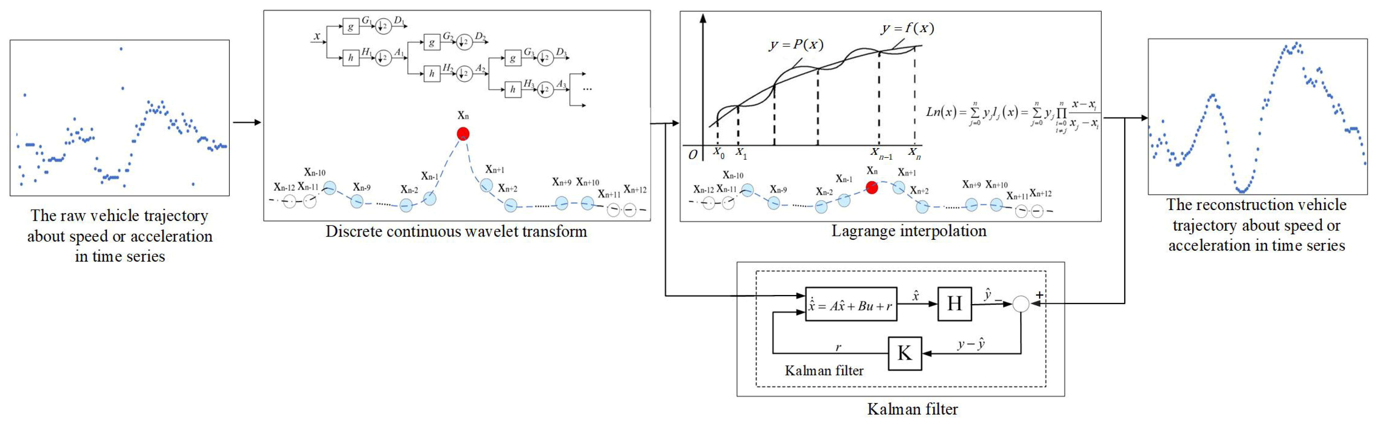
3.1. Method Framework for Vehicle Trajectory Reconstruction

The Lagrange-interpolation-based framework for vehicle trajectory reconstruction integrates the discrete continuous wavelet transform, Lagrange interpolation and the Kalman filter (Figure 2). The discrete continuous wavelet (DWT) is a domain analysis method to detect outliers between speed and acceleration in time series. Fifth-degree and cubic Lagrange interpolation polynomials are developed for reconstructing the outlier between speed and acceleration after the outlier identification. It is noted that the red circle in the chain represents the location of the outlier before and after repaired, blue circles represent normal values in the chain, and white circles represent normal values outside the data chain. Finally, the Kalman filter is used to reduce observation noise and obtain smooth vehicle trajectories.

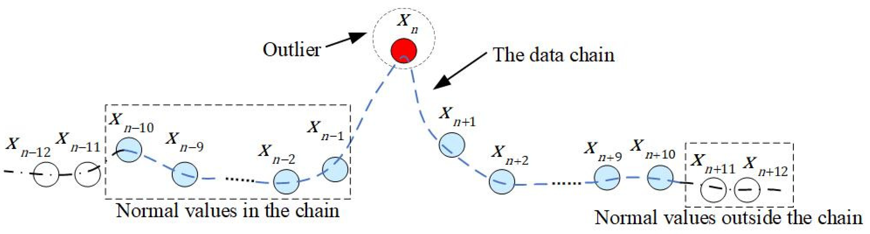
3.2. Outlier Detection

The DWT is a time–frequency domain analysis method of the signal compared with the Fourier transform. It extracts time series features by frequency domain transformation to reduce the dimension of feature space and make features more concentrated [38]. The result of trajectory data is defined by Equations (1)–(3).

$$f\left(x\right)=\frac{1}{\sqrt{M}}{\displaystyle \sum _k{W}_{\varphi }\left(0,k\right){\varphi }_{0,k}\left(x\right)}+\frac{1}{\sqrt{M}}{\displaystyle \sum _{j=0}^{\infty }{\displaystyle \sum _k{W}_{\psi }\left(j,k\right){\psi }_{j,k}\left(x\right)}}$$

(1)

$${\psi }_{j,k}\left(x\right)=2^{\frac{j}{2}}\psi \left(2^{j}x-k\right)$$

(2)

$$DWT\left(j,k\right)=〈f\left(x\right),{\psi }_{j,k}\left(x\right)〉$$

(3)

where $f\left(x\right)$ is the original time domain signal; ${\varphi }_{0,k}\left(x\right)$ is the frequency domain function with position coefficient $k$; and ${\psi }_{j,k}\left(x\right)$ is the wavelet function with position coefficient $k$ and frequency coefficient $j$. $W_{\varphi }\left(0,k\right)$ is the approximation coefficient; $W_{\psi }\left(j,k\right)$ is the detail coefficient.

DWT does not need computers to provide enough RAM in the calculation process and directly discretize the data. According to the collected trajectory data, this paper uses DWT based on the Symlet8 wavelet framework to identify outliers from neighbor data in trajectory data.

3.3. Lagrange Interpolation

Re-estimating the corresponding position data after eliminating the outliers is necessary. Using existing deep learning methods, it is difficult to reconstruct data adaptively and reflect the relationship between independent variables and dependent variables accurately, because the adaptive model is trained based on abnormal trajectory data. This paper finds an approximate function $p\left(x_i\right)$ in a given interval to obtain the expected results. It is defined by Equation (4).

$$p\left(x_i\right)=f\left(x_i\right)i=0,1,2,\cdots ,n$$

(4)

where $x_i$ is the value of ith points in the interval $\left[0,n\right]$, and $f\left(x_i\right)$ is the truth function.

It is noted that the expected values are different when different interpolation functions are selected, according to different bases and constraints in linear space. Lagrange interpolation is a special polynomial interpolation method for solving a class of polynomial problems with given point values. It can choose appropriate estimation scales based on the different characteristics of the data, compared with the mean interpolation method [39]. Equation (5) shows how the method is used to re-estimate the removed outliers of speeds and accelerations at any time.

$$Ln\left(x\right)={\displaystyle \sum _{j=0}^n{y}_j{l}_j\left(x\right)}={\displaystyle \sum _{j=0}^n{y}_j}{\displaystyle \prod _{\begin{array}{l}i=0\\ i\ne j\end{array}}^n\frac{x-x_i}{x_j-x_i}}$$

(5)

where $l_j\left(x\right)$ is the Lagrange interpolation basis function of degree $n$.

After outliers are identified and eliminated, the method re-estimates the value of any position within a given interval based on n + 1 different interpolation points. The paper uses a number of data to construct an approximate function and obtain optimal parameters with the least given adjacent data, and the data called a data chain (Figure 3) contain outliers and twenty neighbor data.

The paper uses the adjacent data in data chains to construct a Lagrange interpolation polynomial and performs a lot of experiments to re-estimate outliers. It finds that the re-estimated speed values obtained from the fifth-degree Lagrange interpolation polynomial are the closest to the empirical vehicle trajectory data, and the convergence calculation of the method takes less time. It is noted that there must be at least three data points on both sides of a data chain when establishing the polynomial. If there are less than thirteen data points between two outliers, the method should merge two neighbor chains into one chain. When there are less than three data points outside the chain, this paper discusses two cases: (1) When there is at least one data point at the boundary of the chain, the neighbor data can be obtained from the other side of the chain to supplement data. (2) When there are no data points at the boundary of the chain, the chain should be deleted. Compared with the abnormal speed, the acceleration has less impact on the neighbor data, the paper finds that the cubic Lagrange interpolation polynomial is more suitable for re-estimating acceleration.

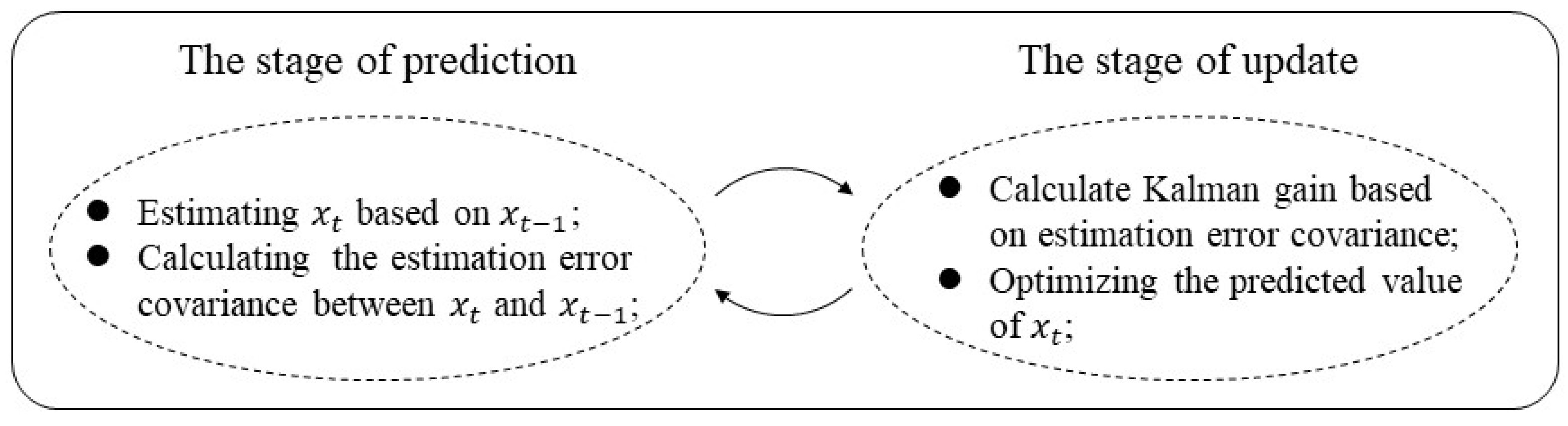
3.4. Filter Denoising

Noise data impact data analysis and calculation. The Kalman filter is used to estimate the state of a dynamic system according to the joint distribution of observed data at different times [40]. Compared with the single observation estimation method, it establishes a state space model for discrete stochastic systems through state equations and observation equations. The method can be defined by Equations (6) and (7).

$$x\left(t+1\right)=\mathsf{\Phi }x\left(t\right)+\mathsf{{\rm B}}u\left(t\right)+\mathsf{\Gamma }w\left(t\right)$$

(6)

$$y\left(t\right)=Hx\left(t\right)+v\left(t\right)$$

(7)

where $x\left(t\right)$ is the vector of the state system; $y\left(t\right)$ is the vector of the observation system; $\mathsf{\Phi },\mathsf{{\rm B}},\mathsf{\Gamma }$ and $H$ represent, respectively, the state transition matrix, control coefficient matrix, input noise coefficient matrix and observation coefficient matrix; $u\left(t\right)$ is input control, initially set to be 0; $w\left(t\right)$ is input white noise; and $v\left(t\right)$ is observation noise.

Kalman filtering removes noise through the prediction and update stages. The filter uses the estimated values of the previous state to obtain the prediction values of the current state in the prediction stage. The prediction formulas are defined by Equations (8) and (9).

$$\widehat{x}{\left(t\right)}^{-}=\mathsf{\Phi }\widehat{x}\left(t-1\right)$$

(8)

$$P{\left(t\right)}^{-}=\mathsf{\Phi }P\left(t-1\right){\mathsf{\Phi }}^T+Q$$

(9)

where $\wedge$ represents the predicted value; $-$ represents the prior value; $P\left(t\right)$ is the estimation error covariance, and $Q$ is the variance matrix of the process noise.

The values of the observation update are calculated with the current observed values and the predicted values from the prediction stage to obtain more accurate estimated values in the update stage. The update formulas are defined by Equations (10) and (11).

$$K\left(t\right)=P{\left(t\right)}^{-}{H}^T{\left(HP{\left(T\right)}^{-}{H}^T+R\right)}^{-1}$$

(10)

$$\widehat{x}\left(t\right)=\widehat{x}{\left(t\right)}^{-}+K\left(t\right)\left(y(t)-H\widehat{x}{\left(t\right)}^{-}\right)$$

(11)

$$P\left(t\right)=\left(I-K\left(t\right)H\right)P{\left(t\right)}^{-}$$

(12)

where $K\left(t\right)$ is Kalman gain, and $R$ is the variance matrix of the observation noise.

The paper uses Kalman filtering to repeat every time in order to denoise and make the initial value of the state estimate equal to the initial value in the previous step (Figure 4). The prediction formulas are used to predict the values at each time, and then the update formulas optimize the estimated values.

4. Results

DWT based on the Symlet8 wavelet framework was used to identify outliers with a judgment threshold. The judgment threshold is [−8 m/s², 5 m/s²] in the limit value of human body bearing and vehicle dynamic performance. The outlier detection formula is defined by Equation (13).

$$S_j^z={\mu }_j\pm z\times {\sigma }_j$$

(13)

where $S_j^z$ is the limit of drift data; ${\mu }_j$ is mean value; ${\sigma }_j$ is standard deviation; $z$ is the coefficient of standard deviation, and it is taken as 1.96 under the 95% confidence interval.

The identification and re-estimation results of the proposed method are shown in Figure 5. The frequency spectrum deeply analyzes the characteristics of the data source system and determines whether there is noise in the vehicle trajectory data.

Figure 5 shows that the wavelet transform based on Symlet8 has better performance in the recognition of outliers. Figure 5b shows that only 4.14% of the acceleration exceeded the limit of human body bearing and vehicle dynamic performance. The re-estimated trajectory data are more gentle than raw data. However, there are still data with frequencies greater than 2 Hz in Figure 5c. It is necessary to reduce the noise interference in the trajectory data.

The Kalman filter is used to reduce noise interference. The noise covariance is set to a constant. The initial value of estimation error covariance $P\left(0\right)$ is 1. It can avoid the value of state estimation always being equal to the initial value. In order to determine the optimal filter parameters, this paper establishes the optimal filter parameter model. It is defined by Equations (14)–(16).

$$\left[Q,R\right]=f\left(R_{signalenergy},acceleration\right)$$

(14)

$$S.T.\left\{\begin{array}{c}\min \left(Rsignalenergy\ge 95\%\right)\\ \left|acceleration\right|\le 5m/s^2\\ \left\{Q,R\right\}\subseteq T\\ T=\left\{0.01,0.02,0.03,\cdots ,1\right\}\end{array}\right.$$

(15)

$$R_{signalenergy}=\frac{{\displaystyle \sum {\left|x\left(t\right)\right|}_{filtered}^2}}{{\displaystyle \sum {\left|x\left(t\right)\right|}_{original}^2}}\times 100\%$$

(16)

where $R_{signalenergy}$ represents the signal energy ratio; $x{\left(t\right)}_{original}$ and $x{\left(t\right)}_{filtered}$ are the state values before and after filtering, respectively. The $Q$ and $R$ are in the interval [0, 1] and increase at intervals of 0.01.

The values of $Q$ and $R$ are 0.05 and 0.15 by iterative calculation. The results of denoising are shown in Figure 6.

Figure 6 shows that the speed of the trajectory data is smoother, and the acceleration value is within the limits. Figure 6c shows that the amplitude of data frequency is less than 1 Hz. The Kalman filter is a recursive filter used to estimate the state of a dynamic system, such as a traffic system or power system. It uses a series of measurements to produce an estimate that is closer to the true state than any individual measurement and can better adapt the geometric curve function input of the Lagrange interpolation polynomial in the processing of vehicle trajectory reconstruction. In order to demonstrate that the Kalman filter has better denoising results in vehicle trajectory reconstruction, the paper compares the denoising results among the different variants of filters, such as the Savitzky–Golay (S-G) filter, symmetric exponential moving average (SEMA) filter and extended Kalman filter (EKF).

Figure 7 shows that the Kalman filter is more sensitive to the observation noise and reduces the error of the re-estimation data in the trajectory data, compared with SEMA and EKF, such as the speed point at the 37th second (see Figure 7a) and the acceleration at the 26th second (see Figure 7b). The S-G filter can greatly remove the noise in the vehicle trajectory (see Figure 7c) but causes excessive denoising in some data.

5. Discussion

This paper uses the 1942nd trajectory in the NGSIM dataset to repair outliers and denoise, compared with the baseline method proposed by Montanino [37]. And it uses three indexes (root mean square error (RMSE), signal-to-noise ratio (SNR) and Pearson correlation coefficient (P)) to demonstrate that the proposed method has good reconstruction results. The three measurements are defined by Equations (17)–(19).

$$RMSE=\sqrt{\frac{1}{N}{{\displaystyle \sum _{i=1}^N\left(S_i-{\widehat{S}}_i\right)}}^2}$$

(17)

$$SNR=10\log \left(\frac{{\displaystyle \sum _{i=1}^N{S}_i{}^2}}{{\displaystyle \sum _{i=1}^N{\left(S_i-{\widehat{S}}_i\right)}^2}}\right)$$

(18)

$$P=\frac{{\displaystyle \sum _{i=1}^N\left(S_i-{\overline{S}}_i\right)\left({\widehat{S}}_i-{\overline{\widehat{S}}}_l\right)}}{{\displaystyle \sum _{i=1}^N{\left(S_i-{\overline{S}}_i\right)}^2{\displaystyle \sum _{i=1}^N\left({\widehat{S}}_i-{\overline{\widehat{S}}}_l\right)}}}$$

(19)

where $S_i$ is the empirical vehicle trajectory data [41]; ${\widehat{S}}_i$ is the reconstructed trajectory data; ${\overline{S}}_i$ and ${\overline{\widehat{S}}}_l$ denote the average of the empirical vehicle trajectory data and the reconstructed trajectory data, respectively; and $N$ is the length of trajectory data.

This paper calculates the three measurements (RMSE, SNR and P) between the baseline method and the proposed method. The results are shown in

Table 2. Comparison of the measurements obtained by the two frameworks.

Index		Baseline Method	Proposed Method
RMSE	Position	0.05	0.035
	Speed	0.08	0.05
	Acceleration	0.43	0.13
SNR	Position	75.13	79.22
	Speed	36.8	44.7
	Acceleration	8.4	12.8
P	Position	1.00	1.00
	Speed	1.00	1.00
	Acceleration	0.77	0.967

.

Table 2 shows that the RMSE of the proposed method is smaller than that of the baseline method. The SNR is greater than that of the baseline method. It shows that this proposed method retains more trajectory information and denoises better. By calculating the average increase percentage of the measurements, it finds that the RMSE of this proposed method is reduced by 45.76%, the SNR is increased by 26.43%, and the P is increased by 25.58% compared with the baseline method.

It is observed that the results of the proposed method are better than those of the baseline framework in Figure 8. The paper uses the acceleration distribution of trajectory data to analyze the acceleration and its proportion. The acceleration distributions among the proposed method, the baseline method and the original trajectory are shown in Figure 9.

Figure 9 shows that acceleration of more than 10% in original data is greater than ±9 m/s². It exceeds the human body bearing limit. The acceleration of the baseline method is more than 20% outside the range of ±5 m/s², and that of the proposed method is in the range of [−3 m/s², 3 m/s²].

The jerk value is the derivative value of acceleration. It indicates the change degree of acceleration in unit time. It is used to analyze whether trajectory reconstruction results are within the limitation of vehicle dynamic and driver driving behavior. The main indexes include the percentage of jerks that are greater than ±15 m/s³, the maximum jerk value, the minimum jerk value, and the percentage that the jerk symbol changes more than once in one second (N). The results are shown in

Table 3. Jerk analysis of trajectory reconstruction results.

Index		Original Trajectory	Baseline Method	Proposed Method
Jerk is greater than ±15 m/s3(%)	mean value	22.93	0.04	0.03
	standard deviation	11.22	0.05	0.23
	range	[4.70, 69.23]	[0.00, 1.75]	[0.00, 4.32]
Maximum jerk	mean value	832.16	33.14	16.83
	standard deviation	712.33	36.21	13.36
	range	[36.33, 8326.91]	[3.96, 193.63]	[0.93, 169.65]
Minimum jerk	mean value	−978.62	−42.12	−13.26
	standard deviation	1021.36	25.69	6.74
	range	[−8795.41, −36.85]	[−121.16, −65.36]	[−86.52, −1.36]
N	mean value	56.32	13.65	7.49
	standard deviation	9.32	7.41	6.34
	range	[42.75, 63.26]	[22.69, 43.77]	[12.34, 37.69]

.

Table 3 shows that the percentage of jerks that are greater than ±15 m/s³ is 22.93% in the original track; the reconstruction results of the baseline method and the proposed method are 0.04% and 0.03%, respectively. The extreme jerks in the proposed paper are [−13.26 m/s³, 16.83 m/s³]. They are much smaller than the processing results of the original data and the baseline method. The N of the proposed method is 7.49%, compared with 13.65% of the baseline framework. It clearly shows that the proposed method has better performance in reconstruction trajectory data.

6. Conclusions

This paper analyzes the existence of outliers and observation noise in the vehicle trajectory data and proposes a processing framework for vehicle trajectory reconstruction. The framework integrates the discrete continuous wavelet transform, Lagrange interpolation and the Kalman filter to identify outliers, re-estimate value after the outliers are eliminated and reduce observation noise in time series. Lagrange polynomial interpolation can be flexibly selected according to the number of trajectory points, which improves the migration of the algorithm. The Kalman filter method with optimized filtering parameters has better results compared with other filters. The proposed method is compared with a baseline method on the NGSIM dataset, and the results indicate that (1) the RMSE obtained by using the proposed method is 45.76% lower than that obtained by using the baseline method. (2) The SNR obtained by using the proposed method is 26.43%. (3) The advantage of the method in terms of the SNR is the largest when Q = 0.05 and R = 0.15. (4) The Pearson correlation coefficient obtained by using the proposed method is 25.58%.

At least three interesting directions can be explored in further studies. Firstly, compared to the trajectory reconstruction based on a geometric curve function, a methodology based on deep learning (such as autoencoders, reinforcement learning, self-supervised learning) could be explored. Secondly, the adaptability of trajectory reconstruction methods should be further verified under complex road conditions. Finally, it is very interesting to combine trajectory reconstruction with urban-delivery route optimization for driverless delivery vehicles.

References

1. Kovvali, V.G.; Alexiadis, V.; Zhang, L. Video-based vehicle trajectory data collection. In Proceedings of the Transportation Research Board 86th Annual Meeting, Washington, DC, USA, 21–25 January 2007. No. 07-0528. [Google Scholar]
2. Xie, K.; Ozbay, K.; Yang, H.; Li, C.G. Mining automatically extracted vehicle trajectory data for proactive safety analytics. Transp. Res. Part C Emerg. Technol. 2019, 106, 61–72. [Google Scholar] [CrossRef]
3. Taylor, J.; Zhou, X.S.; Rouphail, N.M.; Porter, R.J. Method for investigating intradriver heterogeneity using vehicle trajectory data: A dynamic time warping approach. Transp. Res. Part B Methodol. 2015, 73, 59–80. [Google Scholar] [CrossRef]
4. Chen, X.; Zhang, S.; Li, L.; Li, L. Adaptive rolling smoothing with heterogeneous data for traffic state estimation and prediction. IEEE Trans. Intell. Transp. Syst. 2018, 20, 1247–1258. [Google Scholar] [CrossRef]
5. Li, T.; Han, X.; Ma, J. Cooperative perception for estimating and predicting microscopic traffic states to manage connected and automated traffic. IEEE Trans. Intell. Transp. Syst. 2021, 23, 13694–13707. [Google Scholar] [CrossRef]
6. Tsanakas, N.; Ekström, J.; Olstam, J. Generating virtual vehicle trajectories for the estimation of emissions and fuel consumption. Transp. Res. Part C Emerg. Technol. 2022, 138, 103615. [Google Scholar] [CrossRef]
7. Rempe, F.; Franeck, P.; Bogenberger, K. On the estimation of traffic speeds with deep convolutional neural networks given probe data. Transp. Res. Part C Emerg. Technol. 2022, 134, 103448. [Google Scholar] [CrossRef]
8. Lu, X.Y.; Skabardonis, A. Freeway traffic shockwave analysis: Exploring the NGSIM trajectory data. In Proceedings of the 86th Annual Meeting of the Transportation Research Board, Washington, DC, USA, 21–25 January 2007. [Google Scholar]
9. Punzo, V.; Borzacchiello, M.T.; Ciuffo, B. On the assessment of vehicle trajectory data accuracy and application to the Next Generation SIMulation (NGSIM) program data. Transp. Res. Part C Emerg. Technol. 2011, 19, 1243–1262. [Google Scholar] [CrossRef]
10. Coifman, B.; Li, L. A critical evaluation of the Next Generation Simulation (NGSIM) vehicle trajectory dataset. Transp. Res. Part B Methodol. 2017, 105, 362–377. [Google Scholar] [CrossRef]
11. Thiemann, C.; Treiber, M.; Kesting, A. Estimating acceleration and lane-changing dynamics from next generation simulation trajectory data. Transp. Res. Rec. 2008, 2088, 90–101. [Google Scholar] [CrossRef]
12. Ge, Y.; Xiong, H.; Zhou, Z.H.; Ozdemir, H.; Yu, J.; Lee, K.C. Top-eye: Top-k evolving trajectory outlier detection. In Proceedings of the 19th ACM International Conference on Information and Knowledge Management, Toronto, ON, Canada, 26–30 October 2010; pp. 1733–1736. [Google Scholar]
13. Punzo, V.; Borzacchiello, M.T.; Ciuffo, B. Estimation of vehicle trajectories from observed discrete positions and next-generation simulation program (NGSIM) data. In Proceedings of the TRB 2009 Annual Meeting, Washington, DC, USA, 11–15 January 2009. [Google Scholar]
14. Wang, H.; Gu, C.; Ochieng, W.Y. Vehicle trajectory reconstruction for signalized intersections with low-frequency floating car data. J. Adv. Transp. 2019, 2019, 9417471. [Google Scholar] [CrossRef]
15. Venthuruthiyil, S.P.; Mallikarjuna, C.C. Vehicle path reconstruction using Recursively Ensembled Low-pass filter (RELP) and adaptive tri-cubic kernel smoother. Transp. Res. Part C Emerg. Technol. 2020, 120, 102847. [Google Scholar] [CrossRef]
16. Zhou, Y.; Lin, Y.; Ahn, S.; Wang, P.; Wang, X. Platoon Trajectory Completion in a Mixed Traffic Environment Under Sparse Observation. IEEE Trans. Intell. Transp. Syst. 2022, 23, 16217–16226. [Google Scholar] [CrossRef]
17. Hu, X.; Zheng, Z.; Chen, D.; Zhang, X.; Sun, J. Processing, assessing, and enhancing the Waymo autonomous vehicle open dataset for driving behavior research. Transp. Res. Part C Emerg. Technol. 2022, 134, 103490. [Google Scholar] [CrossRef]
18. Zhou, T.; Jiang, D.; Lin, Z.; Han, G.; Xu, X.; Qin, J. Hybrid dual Kalman filtering model for short-term traffic flow forecasting. IET Intell. Transp. Syst. 2019, 13, 1023–1032. [Google Scholar] [CrossRef]
19. Chen, Y.; Yu, P.; Chen, W.; Zheng, Z.; Guo, M. Embedding-based similarity computation for massive vehicle trajectory data. IEEE Internet Things J. 2021, 9, 4650–4660. [Google Scholar] [CrossRef]
20. Belhadi, A.; Djenouri, Y.; Srivastava, G.; Cano, A.; Lin, J.C. Hybrid group anomaly detection for sequence data: Application to trajectory data analytics. IEEE Trans. Intell. Transp. Syst. 2021, 23, 9346–9357. [Google Scholar] [CrossRef]
21. Sauer, T.; Xu, Y. On multivariate Lagrange interpolation. Math. Comput. 1995, 64, 1147–1170. [Google Scholar] [CrossRef]
22. Liu, S.Y.; Liu, C.; Luo, Q.; Lionel, M.N.; Krishnan, R. Calibrating large scale vehicle trajectory data. In Proceedings of the 2012 IEEE 13th International Conference on Mobile Data Management, Bengaluru, India, 23–26 July 2012; IEEE: Piscataway, NJ, USA, 2012; pp. 222–231. [Google Scholar]
23. Wan, F.; Guo, G.; Zhang, C.; Guo, Q.; Liu, J. Outlier detection for monitoring data using stacked autoencoder. IEEE Access 2019, 7, 173827–173837. [Google Scholar] [CrossRef]
24. Peralta, B.; Soria, R.; Nicolis, O.; Ruggeri, F.; Caro, L.; Bronfman, A. Outlier vehicle trajectory detection using deep autoencoders in Santiago, Chile. Sensors 2023, 23, 1440. [Google Scholar] [CrossRef] [PubMed]
25. Zhao, J.; Yang, X.L.; Zhang, C. Vehicle trajectory reconstruction for intersections: An integrated wavelet transform and Savitzky-Golay filter approach. Transp. A Transp. Sci. 2023, 1–24. [Google Scholar] [CrossRef]
26. Montanino, M.; Punzo, V. Trajectory data reconstruction and simulation-based validation against macroscopic traffic patterns. Transp. Res. Part B Methodol. 2015, 80, 82–106. [Google Scholar] [CrossRef]
27. Wang, J.; Chai, R.; Xue, X. The effects of stop-and-go wave on the immediate follower and change in driver characteristics. Procedia Eng. 2016, 137, 289–298. [Google Scholar] [CrossRef]
28. Fard, M.R.; Mohaymany, A.S.; Shahri, M. A new methodology for vehicle trajectory reconstruction based on wavelet analysis. Transp. Res. Part C Emerg. Technol. 2017, 74, 150–167. [Google Scholar] [CrossRef]
29. Durrani, U.; Lee, C. Calibration and validation of psychophysical car-following model using driver’s action points and perception thresholds. J. Transp. Eng. Part A Syst. 2019, 145, 04019039. [Google Scholar] [CrossRef]
30. Chen, X.; Chen, H.; Yang, Y.; Wu, H.; Zhang, W.; Zhao, J.; Xiong, Y. Traffic flow prediction by an ensemble framework with data denoising and deep learning model. Phys. A Stat. Mech. Its Appl. 2021, 565, 125574. [Google Scholar] [CrossRef]
31. Nithin, M.; Panda, M. Multiple model filtering for vehicle trajectory tracking with adaptive noise covariances. In Proceedings of the Intelligent Computing, Information and Control Systems: ICICCS 2019, Secunderabad, India, 27–28 June 2019; Springer International Publishing: Cham, Switzerland, 2020; pp. 557–565. [Google Scholar]
32. Mahajan, V.; Barmpounakis, E.; Alam, M.R.; Geroliminis, N.; Antoniou, C. Treating Noise and Anomalies in Vehicle Trajectories From an Experiment With a Swarm of Drones. IEEE Trans. Intell. Transp. Syst. 2023, 24, 9055–9067. [Google Scholar] [CrossRef]
33. Abbas, M.T.; Jibran, M.A.; Afaq, M.; Song, W.C. An adaptive approach to vehicle trajectory prediction using multimodel Kalman filter. Trans. Emerg. Telecommun. Technol. 2020, 31, e3734. [Google Scholar] [CrossRef]
34. Zhang, B.W.; Yu, W.G.; Jia, Y.F.; Huang, J.; Yang, D.G.; Zhong, Z.H. Predicting vehicle trajectory via combination of model-based and data-driven methods using Kalman filter. Proc. Inst. Mech. Eng. Part D J. Automob. Eng. 2023, 09544070231161846. [Google Scholar] [CrossRef]
35. Zhao, S.; Chen, W.; Deng, Z.; Liu, W. Trajectory tracking control for intelligent vehicles driving in curved road based on expanded state observers. J. Automot. Saf. Energy 2022, 13, 112. [Google Scholar]
36. Hendawi, A.; Shen, J.; Sabbineni, S.; Song, Y.X.; Cao, P.W.; Zhang, Z.; Krumm, J.; Ali, M. Noise patterns in GPS trajectories. In Proceedings of the 2020 21st IEEE International Conference on Mobile Data Management (MDM), Versailles, France, 30 June–3 July 2020; IEEE: Piscataway, NJ, USA, 2020; pp. 178–185. [Google Scholar]
37. Montanino, M.; Punzo, V. Making NGSIM data usable for studies on traffic flow theory: Multistep method for vehicle trajectory reconstruction. Transp. Res. Rec. 2013, 2390, 99–111. [Google Scholar] [CrossRef]
38. Addison, P.S. The Illustrated Wavelet Transform Handbook: Introductory Theory and Applications in Science, Engineering, Medicine and Finance; CRC Press: Boca Raton, FL, USA, 2017. [Google Scholar]
39. Van, M.P. Hermite interpolation on the unit sphere and limits of Lagrange projectors. IMA J. Numer. Anal. 2021, 41, 1441–1464. [Google Scholar]
40. Welch, G.F. Kalman filter. In Computer Vision: A Reference Guide; Springer: Cham, Switzerland, 2020; pp. 1–3. [Google Scholar]
41. Zhao, J.; Victor, L.K.; Sun, J.; Ma, Z.; Wang, M. Unprotected Left-Turn Behavior Model Capturing Path Variations at Intersections. IEEE Trans. Intell. Transp. Syst. 2023, 24, 9016–9030. [Google Scholar] [CrossRef]
Figure 1. Longitudinal speed of vehicle 1882 in NGSIM dataset.
Applsci 14 01173 g001
Figure 2. The method framework for vehicle trajectory reconstruction.
Applsci 14 01173 g002
Figure 3. The diagram of a data chain.
Applsci 14 01173 g003
Figure 4. The process of the prediction and update of Kalman filter.
Applsci 14 01173 g004
Figure 5. The outlier processing results. (a) shows the speed processing effects. (b) shows the acceleration processing effects. (c) shows the frequency spectrum of acceleration.
Applsci 14 01173 g005
Figure 6. The denoising results. (a) shows the speed processing effects. (b) shows the acceleration processing effects. (c) shows the frequency spectrum of acceleration.
Applsci 14 01173 g006
Figure 7. The comparison of denoising results among four filters. (a) shows the speed processing effects. (b) shows the acceleration processing effects. (c) shows the frequency spectrum of acceleration.
Applsci 14 01173 g007
Figure 8. The comparison of trajectory reconstruction results between two methods. (a) shows the speed reconstruction result of the two methods. (b) shows the acceleration reconstruction result of the two methods. (c) shows the frequency spectrum of acceleration under the two methods.
Applsci 14 01173 g008
Figure 9. The acceleration distribution: (a) distribution between raw data and repaired data by using the proposed method; (b) distribution between raw data and repaired data by using baseline method.
Applsci 14 01173 g009