Article

A Forward−Backward Splitting Equivalent Source Method Based on S−Difference

1
School of Mechanical and Precision Instrument Engineering, Xi’an University of Technology, Xi’an 710048, China
2
Key Laboratory of Bridge Detection Reinforcement Technology Ministry of Communications, Chang’an University, Xi’an 710064, China
*
Author to whom correspondence should be addressed.
Appl. Sci. 2024, 14(3), 1086; https://doi.org/10.3390/app14031086
Submission received: 20 September 2023 / Revised: 5 December 2023 / Accepted: 15 December 2023 / Published: 27 January 2024

Abstract

:
The regularization method has a direct impact on the accuracy of the reconstructed sound field in the process of inverse calculation of near−field acoustic holography using the equivalent source method. To expand the frequency range of sound field reconstruction and improve computational accuracy, a forward-backward splitting equivalent source method based on s−difference was proposed, which uses the ratio of the output results of the broadband acoustic holography algorithm as the regularization parameter. Numerical simulations of single source and coherent source sound fields were conducted under different frequency conditions to analyze the performance of the forward-backward splitting regularization algorithm based on s−difference, and experimental verification was performed. The simulation results show that the proposed method can accurately reconstruct the sound field in a wider frequency range, and has high accuracy in reconstructing the sound field of low−frequency coherent sources. The experimental results demonstrate the accuracy and effectiveness of this method in reconstructing mid−to−low−frequency sound fields.

1. Introduction

Near−field Acoustic Holography (NAH) technology [1] has been widely used for source identification and visualization of spatial sound fields. NAH technology has multiple solving methods [2,3,4], among which the Equivalent Source Method (ESM) [5] is widely used and researched in the NAH field due to its simple model, adaptability to any shaped sound source, and high reconstruction accuracy and computational efficiency.
Based on the ESM theory [6], a relationship formula between equivalent source strength and measured sound pressure was established. By making the measured sound pressure on the hologram surface equal to the sound pressure generated by the equivalent source, the equivalent source strength can be solved. In practical engineering applications, the sound pressure matrix between the equivalent source surface and the measurement surface is always uncertain due to the limitation of the number of microphones and measurement conditions. To solve this underdetermined problem, Tikhonov et al.’s [7] regularization method is commonly used to find the optimal equivalent source strength. When using this method, the regularization parameter needs to be determined first, and the reconstruction result depends heavily on the accurate selection of the regularization parameter. The commonly used regularization parameter selection methods mainly include the L−curve method and Generalized Cross Validation (GCV) [8,9]. In recent years, compressed sensing technology based on sparse regularization has been widely used in the field of image processing [10,11]. Sun et al. [12] solved the non−convex regularization function by analyzing the difference between the penalty function and the truncation function to solve the sparse recovery problem. Chardon et al. [13] combined sparsity and compressed sensing theory with near−field acoustic holography, and used the CVX convex optimization toolbox in MATLAB to solve the norm problem. Suzuki et al. [14] proposed establishing a monopole and dipole point source model and developed a specific iterative solver to achieve sparsity by using “norm” for solution vectors. However, it was used for long-distance measurement and focused on high−frequency signals. M Tebolle et al. [15] proposed the Iterative Shrinking Threshold Algorithm (ISTA), which has a simple iterative format but a slow convergence rate. Hald et al. [16] proposed the Wideband Acoustic Holography (WBH) algorithm, which first defined the residual function, and then used a two−step iterative method to solve the sparse solution of the equivalent source amplitude value, which has high reconstruction accuracy only in the mid−to−high−frequency range. Huang et al. [17] proposed combining high−order beamforming with an improved fast iterative shrinkage threshold equivalent source method, which can identify smaller sound source main lobes. After that, Hald [18] elaborated on the principles of five commonly used iterative algorithms, including ISTA, derived their formulas, and compared their respective advantages and applicable frequency ranges through numerical simulation analysis and experimental verification. Based on the above content, a forward-backward splitting (FBS) algorithm for the s−difference of equivalent source method near−field acoustic holography was proposed. The optimal solution formula of Tikhonov regularization was used as the input parameter for the FBS algorithm, and the step size was corrected in each iteration process. The s−difference truncation adjustment strategy was introduced to make it approach the optimal solution of the objective function. The FBS algorithm can expand the applicable frequency range of the sound field reconstruction and ensure its reconstruction accuracy and algorithm reliability.
In this paper, the near−field acoustic holography method of the sparse equivalent source method is further investigated through a series of methods such as theoretical formula derivation, simulation, and experimental verification. A forward-backward splitting algorithm (FBS) based on s−differential is proposed in Section 2. The basic principle of the algorithm is first introduced and the solution procedure is derived. In Section 3, several common regularization algorithms for solving the equivalent source strength are introduced and compared with the proposed algorithm by taking single and coherent sources as the research objects, and the performance of sound field reconstruction is simulated and analyzed, and in Section 4, we take the single source and the coherent source as the experimental objects, collect the sound pressure signal of the single loudspeaker through the microphone, respectively, and substitute the regularization algorithm of FBS with s−difference to optimize the processing to obtain the optimal equivalent source strength suitable for a wider range of frequency bands, so as to reconstruct the acoustic field and validate the validity and stability of the algorithm through the reconstructed surface acoustic pressure cloud diagram.

2. Forward-Backward Equivalent Source Method Based on S−Difference

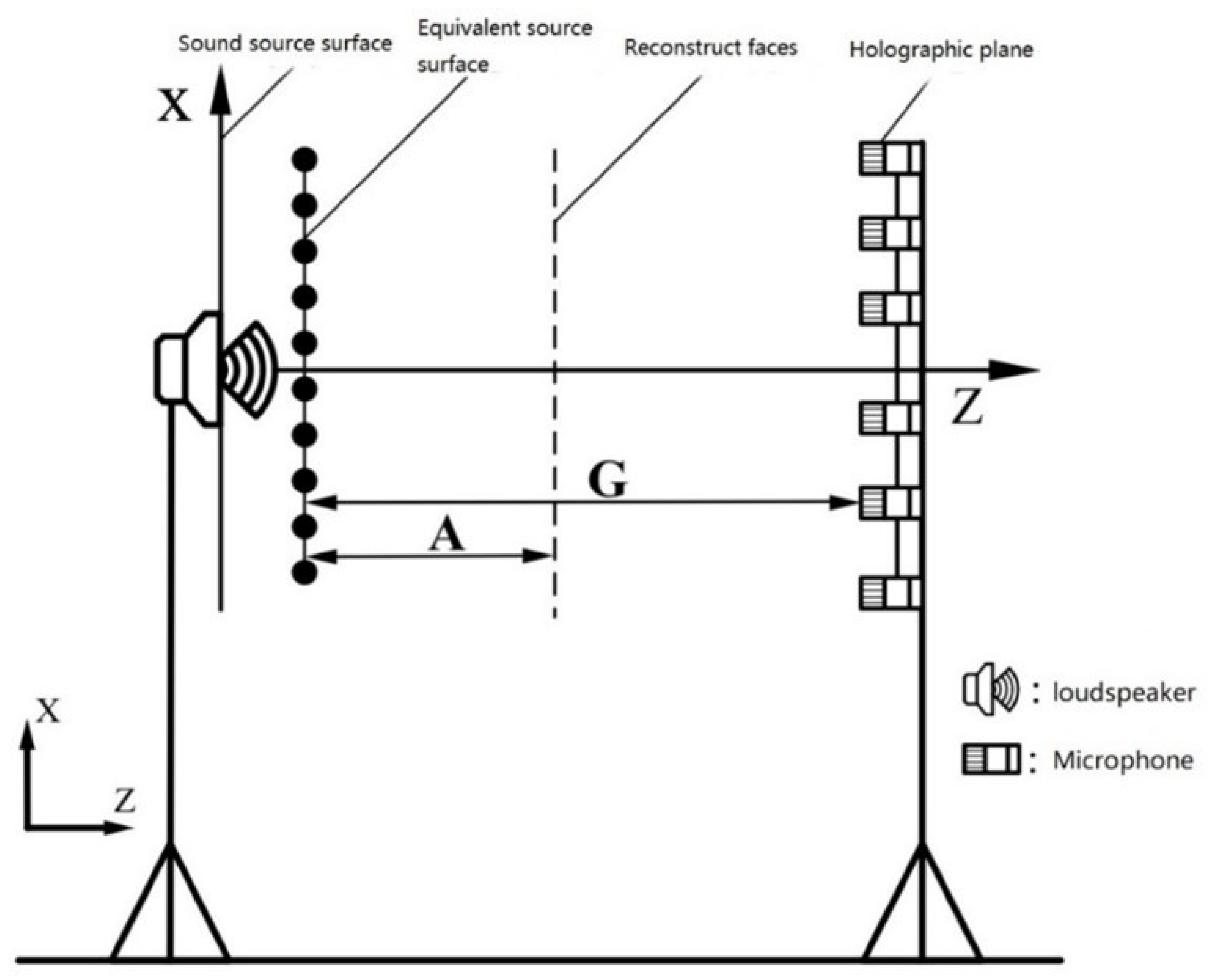
2.1. Basic Principles of Equivalent Source Method

According to the basic principle of equivalent source method near-field acoustic holography, the sound field arrangement is shown in Figure 1, which includes the arrangement of the microphone array, sound source, equivalent source surface, and reconstructed surface. The equivalent source surface can be either a plane or a surface surrounding the sound source. In the equivalent source method, no a priori knowledge is required to use planar equivalent source surfaces. Because the propagation direction of the sound waves on the plane equivalent source surface is known, the equivalent source method can decompose the real sound source on the plane equivalent source surface into a superposition of multiple equivalent sound sources, and the positions and sound pressures of these equivalent sources can be determined more easily. However, to adopt the spherical equivalent source surface, it is necessary to know the location of the sound source in advance and set the spherical equivalent surface at the location of the sound source. Compared with the spherical equivalent source surfaces, the use of planar equivalent source surfaces can make the simulation and modeling more flexible. In this paper, a plane equivalent source surface consisting of a rectangular grid will be used.
Assuming that N equivalent sources are distributed on the equivalent source plane and M microphones are placed on the holographic plane, the sound pressure vector at the m-th measuring point can be expressed as:
p ( m ) = n = 1 N g r m r n q n
where g r m r n represents Green’s function in the free field. The transfer function from the NTH equivalent source to the MTH measurement point can be expressed as:
g ( r m | r n ) = e j k r m n 4 π r m n
where k = 2 Π f / c is the wave number (unit: rad/m). f is frequency, c is velocity, j 2 = 1 , and r m n is the distance from the equivalent source to the microphone and is the determining factor in the relationship between holographic surface sound pressure, equivalent source strength, and transfer matrix, which can be expressed in matrix form:
p = Gq
where G ( M × N ) is the transfer matrix between the equivalent source plane and the holographic plane, p ( M × 1 ) is the complex sound pressure column vector measured by four rows of microphone array, and q ( N × 1 ) is the equivalent source strong column vector.
In practical engineering applications, the number of measurement points is often limited by measurement conditions and costs, resulting in fewer measurement points than equivalent sources, that is, M < < N ; this disparity leads to ill−posed problems when solving Equation (3) for the inverse problem. This inverse problem is flawed because it attempts to reconstruct the evanescent wave part that is away from the sound source surface. The noise present in the measurement process can affect the accuracy of the results, so a regularization method was used to overcome this limitation during the solving process, which helps to improve the accuracy of sound field reconstruction.

2.2. Forward and Backward Splitting (FBS) Regularization Method for S−Difference

The forward and backward splitting algorithm was initially applied in the domain of image restoration. In this section, we modify the regularization parameter in the FBS algorithm and introduce an s−difference adjustment strategy to solve the objective function under the norm constraint. This modification was aimed at improving the accuracy of the algorithm.
In the reconstruction process of image restoration and other practical applications, the l 0 non−convex regularization of the norm has more advantages than the l 1 norm; therefore, we introduce the l 0 constraint problem, expressed as:
min x ϕ ( x ) s u b j e c t t o x 0 s
Firstly, we represent the l 0 constraint problem as the difference between the function R ( x ) and the corresponding s truncation function R ( x s ) , where x s is the best S-term approximation of x . Then, the regularization of S−difference R ( x ) R ( x s ) type is used to solve the unconstrained lowest slide problem. Finally, the closed-form solution is derived from the proximal operator of R ( x ) R ( x s ) and common R ( x s ) .
The l 0 constraint problem is expressed as the difference of convex functions as follows:
x 0 s x 1 x s = 0
where s 1 , 2 , , N , x s represents the sum of the absolute values of the first s larger elements in the vector, also known as the maximum s−norm (or CVaR−norm) [19].
x s : = x π x ( 1 ) + x π x ( 2 ) + + x π x ( s )
where x π x 1 the absolute value of the I th largest element in the vector x R N , so x π x 1 x π x 2 · · · x π x N . Define its set Γ x s = π x ( 1 ) , π x ( 2 ) , , π x ( s ) , and Γ x 1 Γ x 2 Γ x N .
Define its set difference by using , Γ x N Γ x s = π x ( s + 1 ) , π x ( s + 2 ) , , π x ( N ) .
Let x s be defined as the best S−term approximation of the vector x. By using the x π x i definition, we have:
x i s = x i , i f i Γ x s 0 , i f i Γ x N Γ x s

2.3. Forward-Backward Splitting (FBS) Algorithm

First, under the framework of sparse regularization theory, the l 1 norm is used to conduct sparse constraints on the equivalent source intensity vector, and the optimization process can be expressed as:
min i m i z e q q 1 s u b j e c t t o P G q 2 δ
The above equation can be converted into a function minimization problem:
min x P N F ( q ) = ϕ ( q ) + ρ P ( q )
Based on this, we will use FBS to approximate the unconstrained minimization problem and derive the closed-form solution for the proximal operator of P ( q ) [20,21]; this makes the FBS more effective.
Each iteration of forward−backward splitting applies gradient descent of ϕ ( q ) .
q [ k + 1 ] = p r o x β ρ P ( q [ k ] β ϕ ( q [ k ] ) )
β > 0 is the search step size.
Order x * is the optimal solution of the near−end operator, namely x * = p r o x ρ P ( y ) , when R ( q ) = q 1 , P ( q ) = q 1 q s 1 . Then, solve q * as:
q i * = y i , i Γ y s s h r i n k ( y i , ρ β ) i Γ y N Γ y s
where s h r i n k ( y i , ρ β ) represents a soft contraction operator. Γ y s = π y ( 1 ) , π y ( 2 ) , , π y ( s ) and π y ( j ) is the jth maximum amplitude of y, namely y π y ( 1 ) y π y ( 2 ) y π y ( N ) .
s h r i n k ( y i , ρ β ) = s i g n ( y i ) max y i ρ β , 0
The WBH algorithm utilizes an iterative solver to approximate a sparse solution for the equivalent source strength vector. First of all, the residual value r is defined.
r ( q ) = p G q
Secondly, the minimized residual quadratic function F is defined as:
F ( q ) = 1 2 r ( q ) 2 2
Because function F is quadratic differentiable, the optimal solution of the residual function F ( q ) is calculated by a two−step method, including the steepest descent step and the threshold step in each iteration.
We will use a certain proportion of the output values from WBH as the regularization parameter for threshold filtering in FBS. According to a large amount of simulation data, when the value of the regularization parameter for threshold filtering in the FBS is taken to be between 0.05 times and 0.5 times the maximum value of the WBH, ρ [ 0.05 × max ( q w ) , 0.5 × max ( q w ) ] , the effect of reconstruction is good and stable, where max ( q w ) , the regularization parameter, is chosen by taking the absolute maximum value of the equivalent source amplitude vector calculated by WBH. The main reason for using this parameter selection method is that the WBH algorithm is efficient and accurately outputs the amplitude of the equivalent source strength over a wide frequency range.
When the prior sparse range parameter s is unknown, introduce a new adjustment strategy to adapt to each iteration: s [ k + 1 ] = s i z e ( f i n d ( q [ k ] min q π x ( s [ k 1 ] ) [ k 1 ] , δ ) ) , where δ > 0 .
In summary, the LMS algorithm consists of two main processes: filtering and adaptive adjustment. The specific steps are as follows:
(1) Input transfer matrix G and A of equivalent source model;
(2) Measure the sound pressure column vector p ( M × 1 ) , and the equivalent source intensity column vector q ( N × 1 ) ;
(3) Through the L−curve method [22], select appropriate regularization parameters, use Tikhonov to regularize the optimal solution formula: q T i k = G H G + λ I 1 G H p , calculate its equivalent source strength, recorded as q T i k , and WBH calculates the equivalent source intensity, which is recorded as q w ;
(4) Set up q k = q 0 = q T i k , Δ D = 10 , ε = 10 6 , ρ = [ 0.05 × max ( q w ) , 0.5 × max ( q w ) ] ;
(5) Initial truncation condition: t r u n _ x = max ( q T i k ) / Δ D ; if it is greater than the truncation value, q k s = q k , and if it is less than the truncation value, q k s = 0 ;
(6) Initialization: k = 1 , negative gradient vector w k = G T ( G q k p ) , step τ = w k T w k / G w k T G w k ; y k = q k β w k ;
(7) Calculate the median cutoff value t r u n _ y = s i z e ( f i n d ( y k min ( t r u n _ x , δ ) ) ) ; if it is greater than the truncation value, q k + 1 = y k , and if it is less than the truncation value, q k + 1 = s i g n ( y k ) max ( y k ρ β , 0 ) ;
(8) Calculate output truncation value t r u n _ z = s i z e ( f i n d ( q k min ( t r u n _ y , δ ) ) ) ; if it is greater than the truncation value, q k + 1 s = q k + 1 , and if it is less than the truncation value, q k + 1 s = 0 ;
(9) If F q k + 1 F q k / F q k ε or k > k max , finish;
(10) q k = q k + 1 , q k s = q k + 1 s , t r u n _ x = t r u n _ z , k = k + 1 ; output the best equivalent source intensity value and end the cycle;
(11) Output reconstructed surface sound pressure: P R = A q k + 1 ;
Input: transfer matrix G and A of equivalent source model.
Output: the best equivalent source intensity q value.

3. Numerical Simulations

In this section, simulation analysis is conducted for two types of sound sources: single source and coherent source. Firstly, the Tikhonov regularization method, WBH, ISTA, and FBS are used to reconstruct the sound field, and reconstruction error analysis is performed. A pulsating sphere source with a radius of 0.01 m is used as the target sound source, with a vibration velocity of 2.5 × 10⁻² m/s, a sound speed of 340 m/s, and an air density of 1.29 kg/m3. For all subsequent simulations, the holographic plane is located 0.1 m away from the sound source plane to meet the near-field measurement requirement. The reconstruction plane is located 0.02 m away from the sound source plane to better restore the radiation sound field of the target sound source. The equivalent source plane is located 0.001 m away from the sound source plane to optimally represent the actual sound source. The four planes mentioned in the simulation are all in the same coordinate system. The equivalent source plane adopts a 21 × 21 grid with a grid spacing of 0.05 m. The reconstruction plane adopts a 41 × 41 grid with a grid spacing of 0.02 m. A rectangular array of 36 channels is used for near−field sound pressure measurement, and the arrangement of microphones and sound source positions is shown in Figure 2, which is the most suitable configuration for collecting noise generated by automotive components using a wheel array in practical engineering applications. The reconstruction error is calculated using Equation (15). A 36−channel rectangular microphone array was arranged on the holographic surface, and the simulations were all performed in matlab2018 on a computer with Windows 10 (AMD Ryzen 5 2600X processor, 3.60 GHz, 16.00 GB RAM).
In order to quantitatively analyze the reconstruction accuracy of the sound field, the reconstruction error calculation formula is used. Accuracy, the reconstruction error, is calculated as follows:
e r r = i = 1 N p i p ¯ i 2 / i = 1 N p ¯ i 2 × 100
where p ¯ i and p i are the theoretical and reconstructed sound pressure values on the reconstructed surface. The smaller the e r r value, the higher the reconstruction accuracy.

3.1. Single Source Simulation

The purpose of the single-source simulation is to compare four algorithms—Tikhonov regularization, WBH, ISTA and FBS—for sound field reconstruction analysis under a single source. The coordinates of the sound source were (0, 0, 0,) m, and the distance from the holographic surface was set to 0.1 m. Random noise was added to the microphone sound pressure data at a level of 15 dB below the average sound pressure of the microphone, while the dynamic display range was set to 15 dB.
Figure 3 shows the sound pressure level diagrams of the theoretical values on the reconstruction plane, as well as the results calculated by Tikhonov regularization, WBH, ISTA, and FBS algorithms for a single sound source at 200 Hz and 2500 Hz. At 200 Hz, Tikhonov regularization produces a larger hot zone at the sound source location, while WBH, ISTA, and FBS algorithms gradually produce a hot zone that tends toward the center of the sound source, with good recognition performance. At 2500 Hz, all four algorithms produce a concentrated hot zone, and can accurately identify the sound source. The sound pressure cloud maps of several algorithms show that the range of the hot zone is reduced compared with that of 200 Hz, and the sound source identification resolution is improved.
Figure 4 shows the reconstructed sound pressure amplitude of a single sound source in the middle row of the reconstruction plane. At 200 Hz, all algorithms except for FBS have a reconstructed sound pressure amplitude far from the theoretical value, but FBS maintains its high reconstruction accuracy at low frequencies. At 2500 Hz, the amplitude curve of the reconstructed sound pressure in the middle plane calculated by WBH, ISTA, and FBS algorithms matches the theoretical curve, and all algorithms can achieve high−precision sound field reconstruction. The amplitude plot shows that the reconstructed sound pressure peaks of the FBS algorithm are closer to the theoretical sound pressure values, and the reconstruction accuracy is higher than that of the FBS algorithm. The amplitude plot shows that the reconstructed sound pressure peaks of the FBS algorithm are closer to the theoretical sound pressure values, which maintains a high reconstruction accuracy. When the source frequency is 2500 Hz, except for the traditional Tikhonov regularization, which still fails to reconstruct the sound field, the other four algorithms can reconstruct the sound field.
According to Equation (15), Figure 5 shows the reconstruction error curves for a single source in the entire analyzed frequency band from 200 to 2500 Hz, with the frequency sampling points of each curve spaced 50 Hz apart, and the error values averaged over 10 calculations. Overall, WBH, ISTA, and FBS algorithms can reconstruct the sound field more stably than the Tikhonov regularization method. Except for the traditional Tikhonov regularization, the remaining three algorithms maintain more satisfactory reconstruction performance throughout the analyzed frequency band. The three algorithms, WBH, ISTA, and FBS, have good reconstruction accuracy in the middle−frequency and high−frequency bands from 1000 Hz to 2500 Hz, and the reconstruction errors are kept below 20%. Compared with WBH and ISTA, the FBS algorithm maintains higher reconstruction accuracy in the low−frequency band from 200 to 500 Hz, and the reconstruction errors in the whole frequency range are kept below 10%, which broadens the frequency range and ensures the best sound field reconstruction performance.

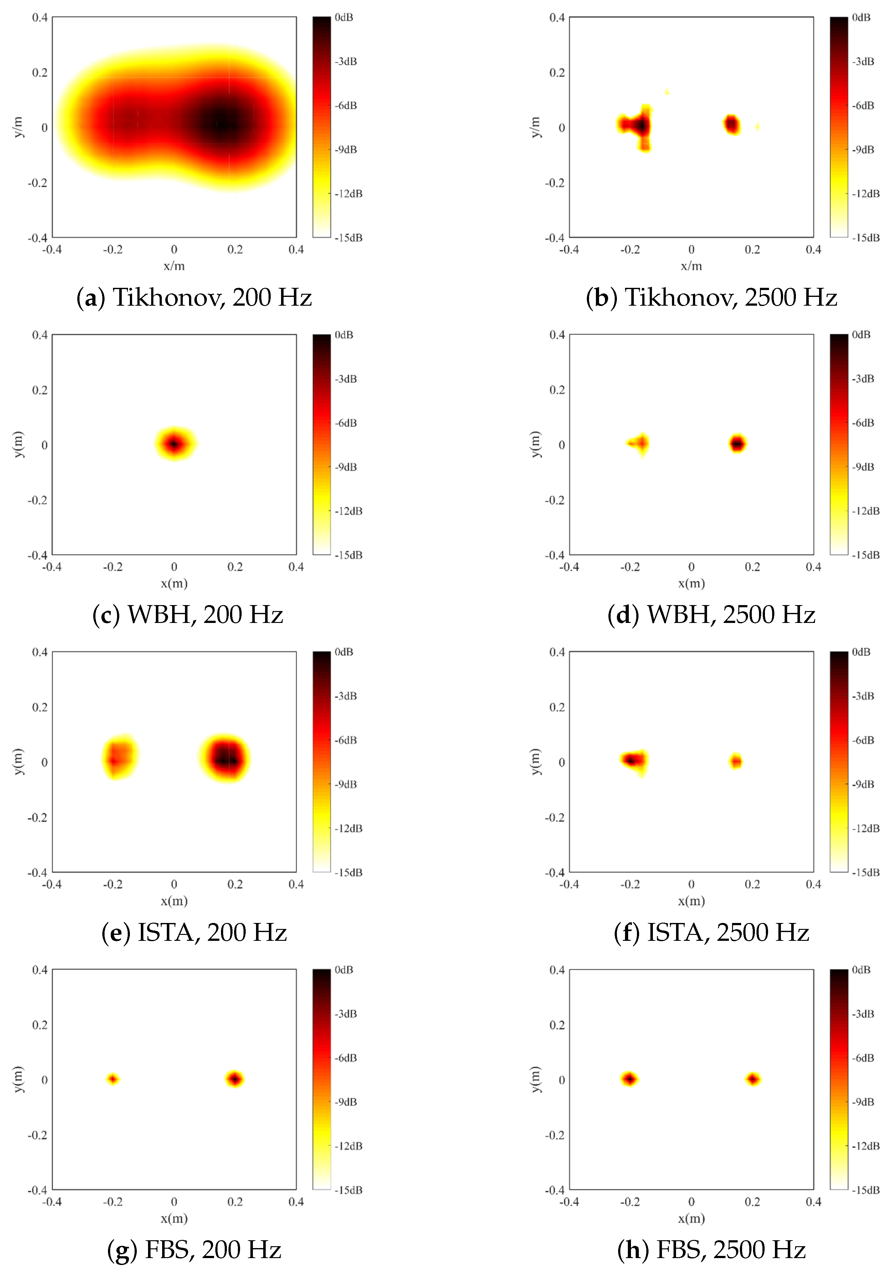
3.2. Coherent Sound Source Simulation

This section analyzes the reconstruction performance of the four regularization methods mentioned above for coherent sound sources. The simulation settings for both coherent and single sound sources are the same. Sound sources are symmetrically distributed about the Y−axis and are separated by 0.4m along the X−axis, then the sources are located at the following coordinates: (0.2, 0, 0) m and (−0.2, 0, 0) m.
Figure 6 shows the reconstructed sound pressure amplitude of the coherent sources in the middle row of the reconstruction plane. At the source frequency of 200 Hz, the peak value of the sound pressure amplitude of the coherent sound source of the intermediate row is close to the theoretical value, which can accurately reconstruct the sound field. At the frequency of 2500 Hz, the sound pressure amplitude calculated by WBH, ISTA, and FBS is almost identical to the theoretical value, which can achieve sound field reconstruction.
The sound field reconstruction results of coherent sound sources at 200 Hz and 2500 Hz are shown in Figure 7. At the coherent source frequency of 200 Hz, the two real sources in the Tikhonov regularization method are covered by larger hot zones and cannot be accurately identified; WBH identifies the number and position of the sources incorrectly. In contrast, ISTA and FBS can clearly identify the two sources, and the hot zone generated by FBS is more concentrated at the source position. At a frequency of 2500 Hz, the hot zones of these five algorithms can clearly indicate the positions of the given sources and perform sound field reconstruction. The identification effects of ISTA and FBS are relatively close, and the sound pressure level graph fits well with the theoretical sound pressure level graph in hot zone size.
The reconstruction error of the coherent sources is shown in Figure 8. It can be seen that the reconstruction error value of Tikhonov regularization in the full frequency band is mainly concentrated in the range of 40−50%; the reconstruction fails and the algorithm is no longer applicable. There exists a conversion frequency for the WBH algorithm, and according to the analysis of the curve direction, it is concluded that the conversion frequency is close to 1000 Hz; when the computation frequency is higher than the critical value, the overall error is kept under 15%, showing good reconstruction performance. In contrast, the frequency range of the ISTA and FBS algorithms is widened, and FBS is able to reconstruct the sound field in the whole frequency band from 200 to 2500 Hz. The frequency range is broadened, and the error value of FBS in reconstructing the sound field in the whole frequency band from 200 to 2500 Hz is kept below 10%, which shows that the algorithm can reconstruct the sound field stably and accurately. This shows that the algorithm can reconstruct the sound field stably and accurately.

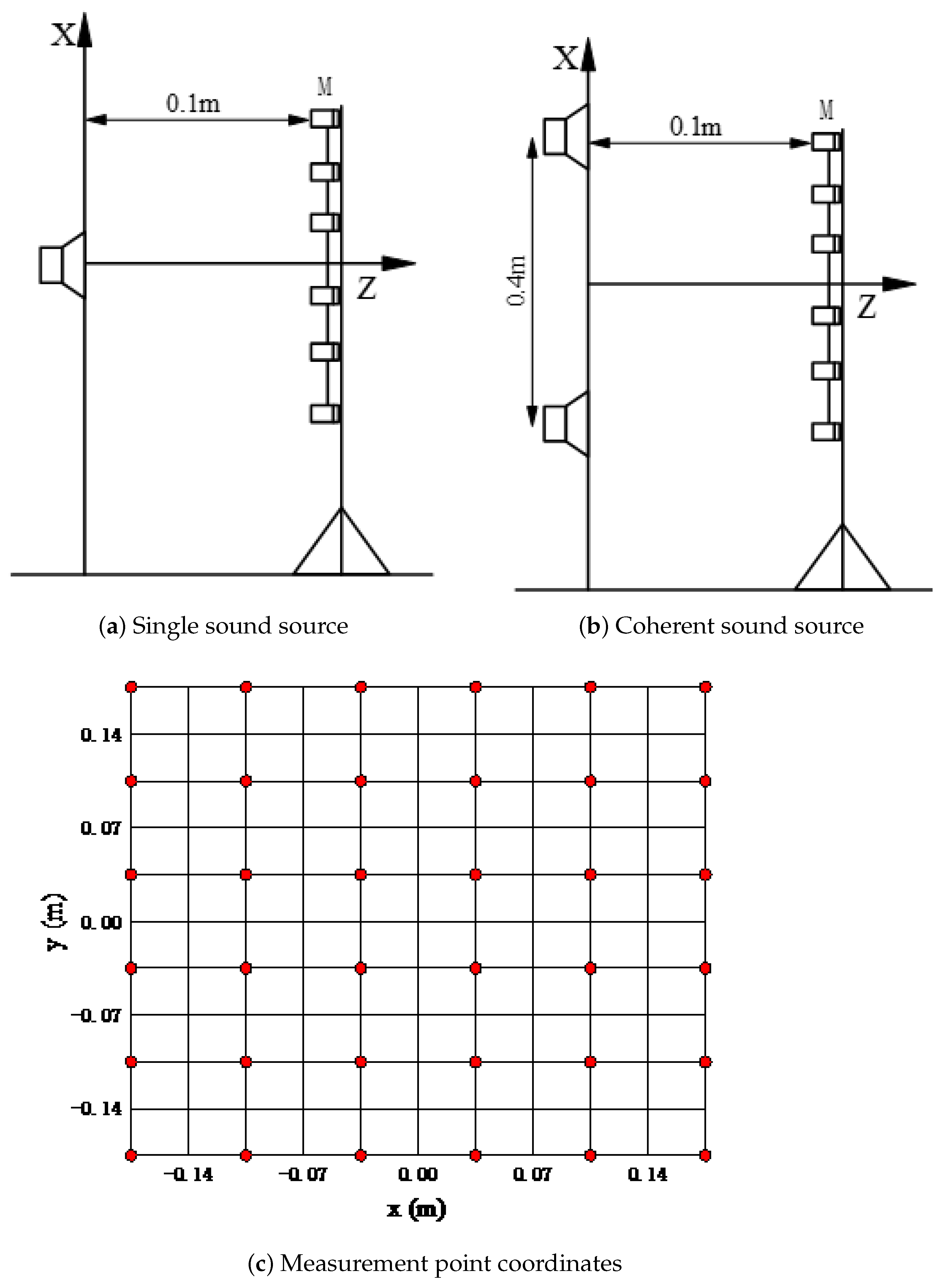
4. Experimental Verifications

4.1. Experimental Procedure

In this section, experiments were conducted to verify the sound field reconstruction effect of the four near−field acoustic holography algorithms mentioned above. This will facilitate further improvement of near−field acoustic holography technology. The improved sparse equivalent source method is more accurate for the identification and location of automobile noise sources, and also provides a reference for suppressing the noise of automobile parts. In the experiment, an 18−channel wheel array with a diameter of 0.38 m from HBK was used for measurement. Data collector and PLUSE Lab Shop Version acquisition software were used to process the time domain sound pressure signal. The microphone position distribution is shown in Figure 9.
The experimental conditions are shown in Figure 10. A single loudspeaker was placed at the origin of the coordinates, taking the center axis of the measurement surface of the microphone array as the reference. The single loudspeaker is arranged on the center axis, with the corresponding coordinates of s0 (0, 0, 0) m, and the distance from the loudspeaker to the measurement surface of the microphone array is 0.1m; the spatial coordinates of the coherent sound sources are s1 (0.2, 0, 0) m and s2 (−0.2, 0, 0) m, respectively. During the experiment, the first step was to ensure that the two speakers were of the same model. The loudspeakers were firstly used to emit sounds with frequencies of 200 Hz and 2500 Hz, respectively, based on the assurance that the two loudspeakers were of the same model, and 2500 Hz, respectively. The sampling frequency was set to 16,384 Hz, and the sampling time was 5s to ensure that the measurement data were stable and valid, and we added 20 dB of random noise during the experiment to ensure the measurement conditions. Through the holographic surface, we collected the time domain signal and exported it to a table data file, and then used the software to process the data of acoustic information. The sound pressure level was used as the output parameter and the display range of the cloud was set to 15 dB with a gradient of 3 dB.

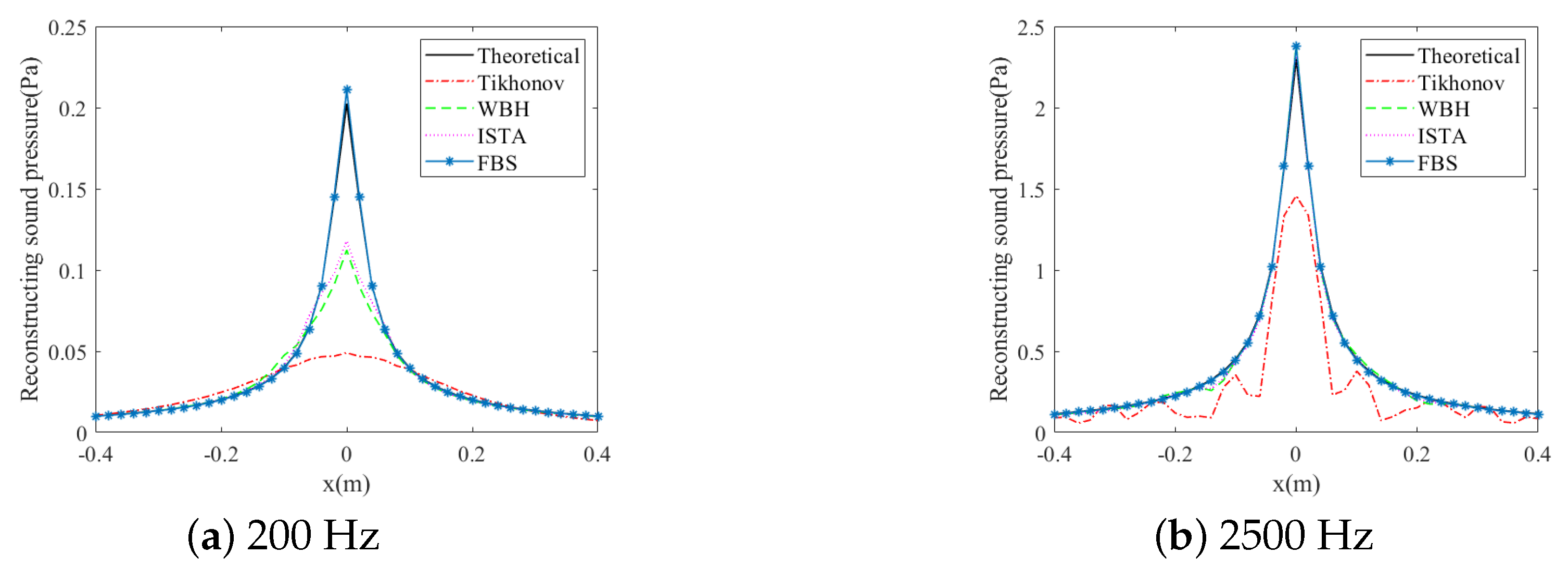
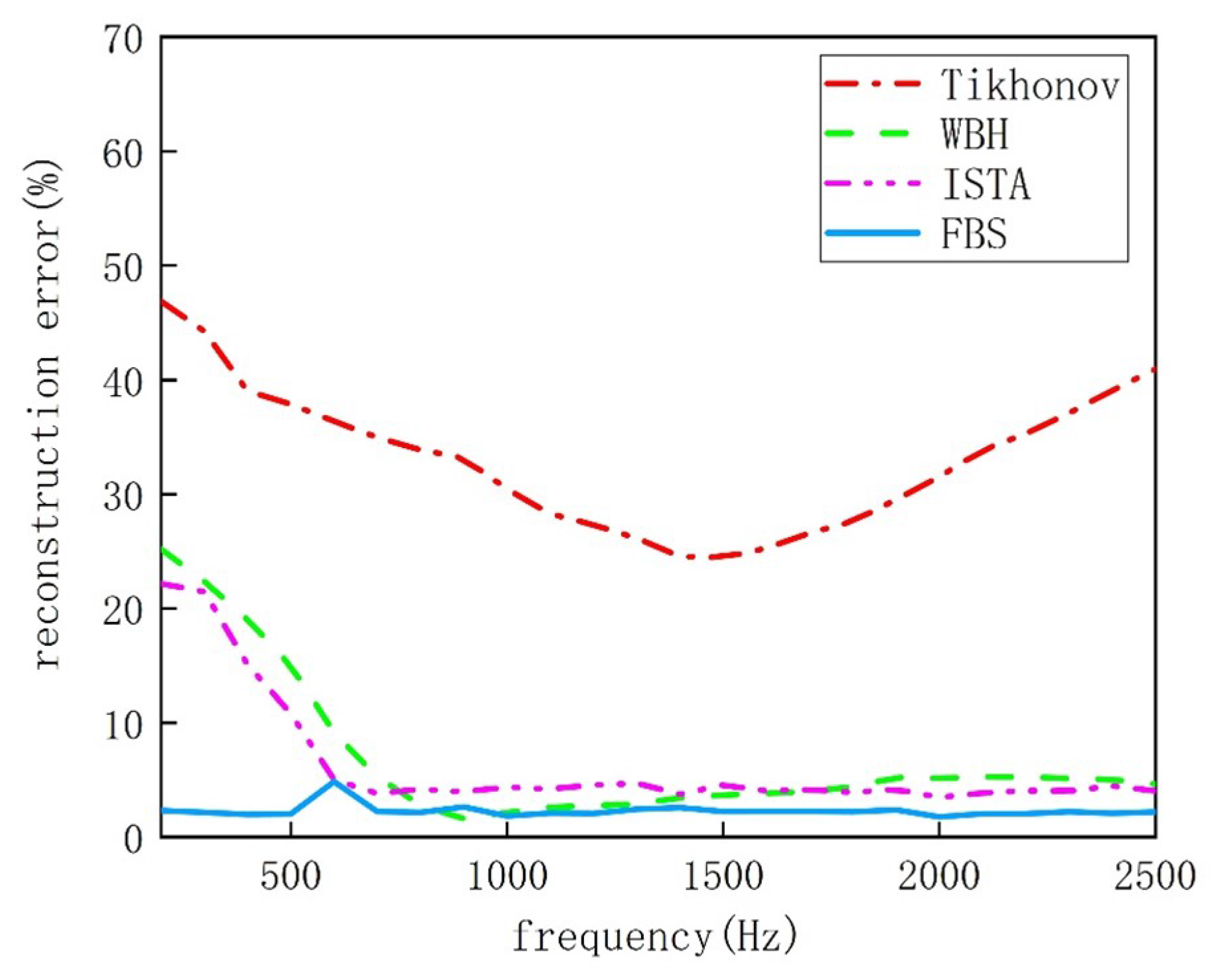
4.2. Experimental Treatment

In the experiment, let the time-domain signal measured by the microphones in the measurement array be P h t . The data processing process starts with obtaining the complex sound pressure at each microphone position in the measurement array. The equation for solving the complex sound pressure is as follows:
A ω = s h , h ω
In Equation (16), s h , h ω is the self-spectrum of the time-domain data P h t at the array measurement points.
The phase is solved as follows:
θ ω = a r g s h , h ω
In Equation (17), arg is the function that takes the phase. According to Equations (16) and (17), the complex sound pressure at the location of the microphone measurement point corresponding to the location of each microphone measurement point in the array can be found.
According to the amplitude and phase of the sound pressure at each measurement point location on the holographic surface, the complex sound pressure at the corresponding location of each microphone can be derived. The reconstruction of the sound field formed by single and coherent sources is performed using the equivalent source method and the s−differential forward−backward splitting (FBS) algorithm, and the reconstructed sound field is shown in Figure 11 and Figure 12. The sound field formed by the single source and coherent sources is reconstructed using the equivalent source method and the s−differential forward−backward split (FBS) algorithm.
Figure 11 is the reconstructed sound pressure level diagram of the single sound source experiment. At the single sound source frequency of 200 Hz, the Tikhonov regularization method produced a large hot zone around the center, resulting in poor reconstruction performance. Although the WBH and ISTA algorithms accurately identified the single source location, a significant hot zone was still visible around the origin coordinates. Only the FBS algorithm produced a smaller hot zone and achieved accurate sound field reconstruction. At the single sound source frequency of 2500 Hz, the hot zones produced by these four regularization algorithms were concentrated at the sound source location, which was consistent with the simulation results, and the reconstruction effect of FBS was the best.
Figure 12 shows the reconstructed sound pressure level diagram of the coherent sound source experiment. It can be seen from the figure below that when the frequency of the coherent sound source is 200 Hz, the sound pressure level cloud map is consistent with the theoretical sound pressure level cloud map, and the hot zone displayed by FBS accurately identified the source location, although the sound pressure amplitude was affected by external experimental conditions. When the frequency of the coherent sound source is 2500 Hz, although the hot zones produced by all four algorithms could deduce the approximate source location, only the FBS two−source hot zone image was close, maintaining high reconstruction accuracy.

5. Conclusions

The near−field acoustic holography based on the equivalent source method is ill−posed, which requires the use of regularization methods to reduce the influence of input errors on the reconstruction accuracy. Due to the limitations of traditional regularization methods, a forward−backward splitting (FBS) algorithm based on s−differential approximation is proposed to approximate the solution, and a closed form solution of s−differential regularization is derived. Numerical simulations show that FBS is superior to Tikhonov regularization in terms of reconstruction accuracy and resolution. Additionally, compared to the ISTA and WBH regularization methods, FBS maintains higher reconstruction accuracy across the entire frequency range of 200–2500 Hz, and produces reconstructed sound pressure peaks that are closer to the theoretical values. The experimental verification of single and coherent sound sources shows that the sound field reconstruction within a wide frequency range of 200–2500 Hz is highly consistent with simulation results and accurately identifies the sound source location while maintaining high reconstruction accuracy, thus validating the effectiveness and stability of this method for reconstructing mid−to−low−frequency sound sources.
Although the s−differential FBS algorithm proposed in this paper is able to accurately locate and identify the position of a single or coherent source in the near field, when the distance between the source plane and the holographic plane becomes large, the algorithm is limited in its ability to accurately reconstruct the radiated sound field at any position. However, when the distance between the source plane and the holographic plane becomes very large, the algorithm is limited in its ability to accurately reconstruct the radiated sound field at any location, and the algorithm should be further optimized for reconstructing the sound field of a long distance source to be better adapted to the holographic distance in subsequent work.
To address the problem that the s−differential FBS algorithm needs to rethreshold the initial iteration when reconstructing the sound field in the low−frequency band, based on numerical simulation, the thresholds in the initial iteration are selected again. Based on numerical simulation and the two−step iterative shrinkage thresholding algorithm, the range of values is roughly determined, while in actual engineering applications, how to accurately select the initial threshold needs to be further explored.

Author Contributions

Conceptualization, J.M. and D.S.; methodology, J.M. and D.S.; software, J.L.; validation, Z.W.; data curation, Z.W.; writing—original draft preparation, J.L.; writing—review and editing, J.M.; funding acquisition, J.M. All authors have read and agreed to the published version of the manuscript.

Funding

This research is supported by the Fundamental Research Funds for the Central Universities, CHD (300102211514, 300102210512).

Institutional Review Board Statement

Not applicable.

Informed Consent Statement

Not applicable.

Data Availability Statement

Data are contained within the article.

Conflicts of Interest

The authors declare that they have no known competing financial interests or personal relationships that could have appeared to influence the work reported in this paper.

References

  1. Maynard, J.D.; Williams, E.G.; Lee, Y. Nearfield acoustic holography: I. Theory of generalized holography and the development of NAH. J. Acoust. Soc. Am. 1985, 78, 1395–1413. [Google Scholar] [CrossRef]
  2. Lee, M.; Bolton, J.S. Patch near-field acoustical holography in cylindrical geometry. J. Acoust. Soc. Am. 2005, 118, 3721–3732. [Google Scholar] [CrossRef]
  3. Steiner, R.; Hald, J. Near-field acoustical holography without the errors and limitations caused by the use of spatial DFT. Int. J. Acoust. Vib. 2001, 6, 83–89. [Google Scholar] [CrossRef]
  4. Chen, L.L.; Shen, X.W.; Liu, C.; Xu, Y.M. Shape optimization analysis of sound barriers based on the isogeometric boundary element method. J. Vib. Shock 2019, 38, 114–120. [Google Scholar]
  5. Koopmann, G.H.; Song, L.; Fahnline, J.B. A method for computing acoustic fields based on the principle of wave superposition. J. Acoust. Soc. Am. 1989, 86, 2433–2438. [Google Scholar] [CrossRef]
  6. Liu, Y.S.; Zeng, X.Y.; Wang, H.T. 3D sound field reconstruction for the enclosed cavity using the multilayer equivalent sources method. Chin. J. Acoust. 2020, 45, 367–376. [Google Scholar]
  7. Williams, E.G. Regularization methods for near-field acoustical holography. J. Acoust. Soc. Am. 2001, 110, 1976–1988. [Google Scholar] [CrossRef] [PubMed]
  8. Chu, Z.; Ping, G.; Yang, Y.; Shen, L. Determination of regularization parameters in near-field acoustical holography based on equivalent source method. J. Vibroeng. 2015, 17, 1976–1988. [Google Scholar]
  9. Xiao, Y. A New Method for Determining Optimal Regularization Parameter in Near-Field Acoustic Holography. Shock. Vib. 2018, 2018, 7303294. [Google Scholar] [CrossRef]
  10. Kim, S.J.; Koh, K.; Lustig, M. An interior-point method for large-scale L1-regularized least squares. IEEE J. Sel. Top. Signal Process. 2007, 1, 606–617. [Google Scholar] [CrossRef]
  11. Lin, Y.; Lee, D.D. Bayesian regularization and nonnegative deconvolution for room impulse response estimation. IEEE Trans. Signal Process. 2006, 54, 839–847. [Google Scholar]
  12. Sun, Y.; Tan, X.; Li, X.; Lei, L.; Kuang, G. Sparse optimization problem with s-difference regularization. Signal Process 2020, 168, 107369. [Google Scholar] [CrossRef]
  13. Chardon, G.; Daudet, L.; Peillot, A.; Ollivier, F.; Bertin, N.; Gribonval, R. Near-field acoustic holography using sparse regularization and compressive sampling principles. J. Acoust. Soc. Am. 2012, 132, 1521–1534. [Google Scholar] [CrossRef] [PubMed]
  14. Uzuki, T. L1 generalized inverse beam-forming algorithm resolving coherent/incoherent, distributed and multipole sources. J. Sound Vib. 2011, 330, 5835–5851. [Google Scholar]
  15. Beck, A.; Teboulle, M. A fast iterative shrinkage-thresholding algorithm for linear inverse problems. SIAM J. Imaging Sci. 2009, 2, 183–202. [Google Scholar] [CrossRef]
  16. Gade, S.; Hald, J.; Ginn, K. Wideband acoustical holography. Sound Vib. 2016, 50, 8–13. [Google Scholar]
  17. Huang, L.S.; Xu, Z.M.; Zhang, Z.F.; He, Y.S. A fast iterative shrinkage threshold sound source identification algorithm and its improvement. Chin. J. Sci. Instrum. 2021, 42, 257–265. [Google Scholar]
  18. Hald, J. A comparison of iterative sparse equivalent source methods for near-field acoustical holography. J. Acoust. Soc. Am. 2018, 143, 3758–3769. [Google Scholar] [CrossRef]
  19. Pavlikov, K.; Uryasev, S. CVaR norm and applications in optimization. Optim. Lett. 2014, 8, 1999–2020. [Google Scholar] [CrossRef]
  20. Combettes, P.L.; Pesquet, J.C. Proximal splitting methods in signal processing. Inverse Probl. Sci. Eng. 2011, 185–212. [Google Scholar]
  21. Pan, Z.Z.; Zhong, Z.; Li, J.; Shi, Y. Compressed sensing reconstruction algorithm based on adaptive acceleration forward-backward pursuit. J. Commun. 2020, 41, 25–32. [Google Scholar]
  22. Lingzhi, L.I. The determination of regularization parameters in planar nearfield acoustic holography. Acta Acust. 2010, 35, 169–178. [Google Scholar]
Figure 1. Schematic diagram of the principle of the equivalent source method. (A represents the distance from the equivalent source surface to the reconstruction surface, and G represents the distance from the sound source surface to the holographic surface).
Applsci 14 01086 g001
Figure 2. Schematic diagram of sound source layout.
Applsci 14 01086 g002
Figure 3. The calculated sound pressure level of single sound source at 200 Hz and 2500 Hz.
Applsci 14 01086 g003
Figure 4. Reconstructed sound pressure amplitude of a single sound source along the middle row of the reconstructed surface.
Applsci 14 01086 g004
Figure 5. Single source reconstruction errors between Tikhonov, WBH, ISTA, and FBS.
Applsci 14 01086 g005
Figure 6. Reconstructed sound pressure amplitude of a single sound source along the middle row of the reconstructed surface.
Applsci 14 01086 g006
Figure 7. Calculated sound pressure level diagram of 200 Hz and 2500 Hz coherent sound sources.
Applsci 14 01086 g007
Figure 8. Coherent source reconstruction errors between Tikhonov, WBH, ISTA, and FBS.
Applsci 14 01086 g008
Figure 9. Microphone array coordinates.
Applsci 14 01086 g009
Figure 10. Experimental conditions.
Applsci 14 01086 g010
Figure 11. Reconstructed sound pressure level diagram of 200 Hz and 2500 Hz single sound source.
Applsci 14 01086 g011
Figure 12. Reconstructed sound pressure level diagram of 200 Hz and 2500 Hz coherent sound sources.
Applsci 14 01086 g012
Disclaimer/Publisher’s Note: The statements, opinions and data contained in all publications are solely those of the individual author(s) and contributor(s) and not of MDPI and/or the editor(s). MDPI and/or the editor(s) disclaim responsibility for any injury to people or property resulting from any ideas, methods, instructions or products referred to in the content.

