1. Introduction
Over the years, car safety tech and crash prevention systems have improved a lot, and this has made active safety tech even better at stopping car accidents [
1]. Efforts to reduce traffic jams and boost overall traffic efficiency have also increased [
2]. Through complete digitization, the vehicles and all the elements related to the transportation system are evolving into sophisticated, interconnected complex-networked mobile computers. In particular, this aspect includes various networked microprocessor-based electronic control units (ECU) that enhance their functions and serve as a foundation for continuous control [
3,
4]. Notably, the real-time estimation of data regarding the changes in vehicle’s velocity components plays a vital role in three key areas:
For what concerns the driving assistance systems, the increasing level of vehicle dependence on software has made complex control systems essential for modern vehicle development.
Advanced safety systems, such as the anti-lock braking system (ABS), traction control system (TCS), and stability control systems, have become common features in modern vehicles [
5,
6]. To guarantee the optimal performance of these vehicle control systems, it is crucial that all the data collected from on-board instruments, combined with insights from predictive models, maintain a high level of quality [
7,
8,
9,
10,
11,
12,
13].
An accurate estimation of the vehicle longitudinal speed [
14], combined with the estimation of the sideslip angle, is crucial for the design and implementation of safety-related control integrated systems. Indeed, the knowledge of the mentioned quantities can be useful for emergency braking, by enabling systems to detect potential collisions and respond promptly; for traction control, by controlling wheel spin, maintaining grip on the road, especially in adverse conditions; and for stability control, for preventing skidding and maintaining control during aggressive maneuvers.
The estimation of a vehicle’s longitudinal velocity and sideslip angle is a crucial topic also in the autonomous driving field [
15]. Indeed, it allows autonomous vehicles to continuously monitor their velocity and direction to adapt both of them appropriately to road conditions. Moreover, thanks to these quantities, the vehicle is able to predict the trajectories, maintaining stability during turns and thereby enhancing overall safety.
Another field of interest for the estimation of a vehicle’s longitudinal velocity and sideslip angle is motorsport. Indeed, accurately estimating tire dynamics requires reliable knowledge of the longitudinal velocity and sideslip angle to determine slip indices [
16]. In addition, these quantities are really useful for selecting the best vehicle setup to ensure the proper use of tires during races. For this aspect, it is also essential to characterize the tires from both a mechanical and thermal point of view [
17,
18,
19], and this is related to the evaluation of the forces acting on the tires and the optimal thermal window of the same. In this way, it is possible to understand how to maximize the best overall vehicle performance, taking into account the tire/road interaction phenomena.
The sideslip angle estimation can be also useful to predict when the vehicle is going to saturate the tires and lose directional stability [
20], allowing for easy identification of understeer and oversteer conditions [
21]. In particular, the estimation of the sideslip angle can be combined with sideslip control, particularly in high-performance and sports driving scenarios. This approach is designed to maintain the vehicle’s sideslip angle within a specific range by employing various controls [
22,
23,
24]. Given the significant relationship between the sideslip angle and the tire’s operating conditions, it plays a critical role as an input for estimating the maximum friction coefficient between the tire’s contact patch and the road surface [
25,
26,
27]. Further, this can also be used to assess tire wear [
28,
29].
Unfortunately, the measurement of the longitudinal velocity and the sideslip angle requires the use of complex and relatively expensive devices. This equipment includes optical sensors, the Global Positioning System, and the inertial platform. Furthermore, these instruments may encounter challenges, such as reflection issues with optical sensors when pointed at reflective surfaces like snow-covered roads, or general failures in the acquisition system.
In addition, in some contexts like motorsport, it is not even possible to use these sensors during the races; then it becomes essential the virtual estimation of both longitudinal velocity and sideslip angle.
According to the methods present in the literature, two main categories of vehicle sideslip angle estimation have been identified: observer-based and neural network-based [
30,
31]. For what concerns the first one, the most famous is the Kalman filter [
32,
33]. In the automotive domain, a multitude of nonlinear Kalman filters have been developed, and they find significant applications, mainly due to the nonlinearity of vehicle dynamics models [
34]. On the other hand, the main obstacle with this approach lies in finding a balance between the complexity of the vehicle model, the quality of results, accuracy, and the computational burden required to achieve real-time sideslip angle estimation. The other category refers to the estimation of the sideslip angle through the use of neural networks (NN), a paradigm of the broader machine learning techniques [
35,
36,
37,
38,
39]. An artificial neural network consists of interconnected neurons communicating through layers, adjusting their structure based on training information [
40]. In recent years, neural networks have gained significance in the automotive industry for estimating variables without specific measuring procedures. This approach offers cost-effective computations, easy algorithm implementation in vehicles, and accurate results, especially in complex real-time control environments. It is important to note that the output of the neural network relies heavily on the data used for training. To achieve accurate generalization, the neural network requires a large amount of reliable data. However, if the network is appropriately trained on a robust and large dataset, it can accurately predict vehicle behavior, even in strongly nonlinear conditions. Moreover, the neural network does not require physical models. On the other hand, as stated, the Kalman filter requires a dependable vehicle dynamic or kinematic model to work. Regarding the sideslip angle estimation, the first type relies on tire models, which can become inaccurate in strongly nonlinear conditions, while the latter type in the Kalman filter tends to become unobservable for low yaw rate values and provide uncertain estimates [
24,
41].
For this reason, starting from previous work of the authors, in which is presented a novel methodology for estimating longitudinal vehicle velocity, this paper extends the approach to evaluate the sideslip angle and integrates the estimates of these two quantities [
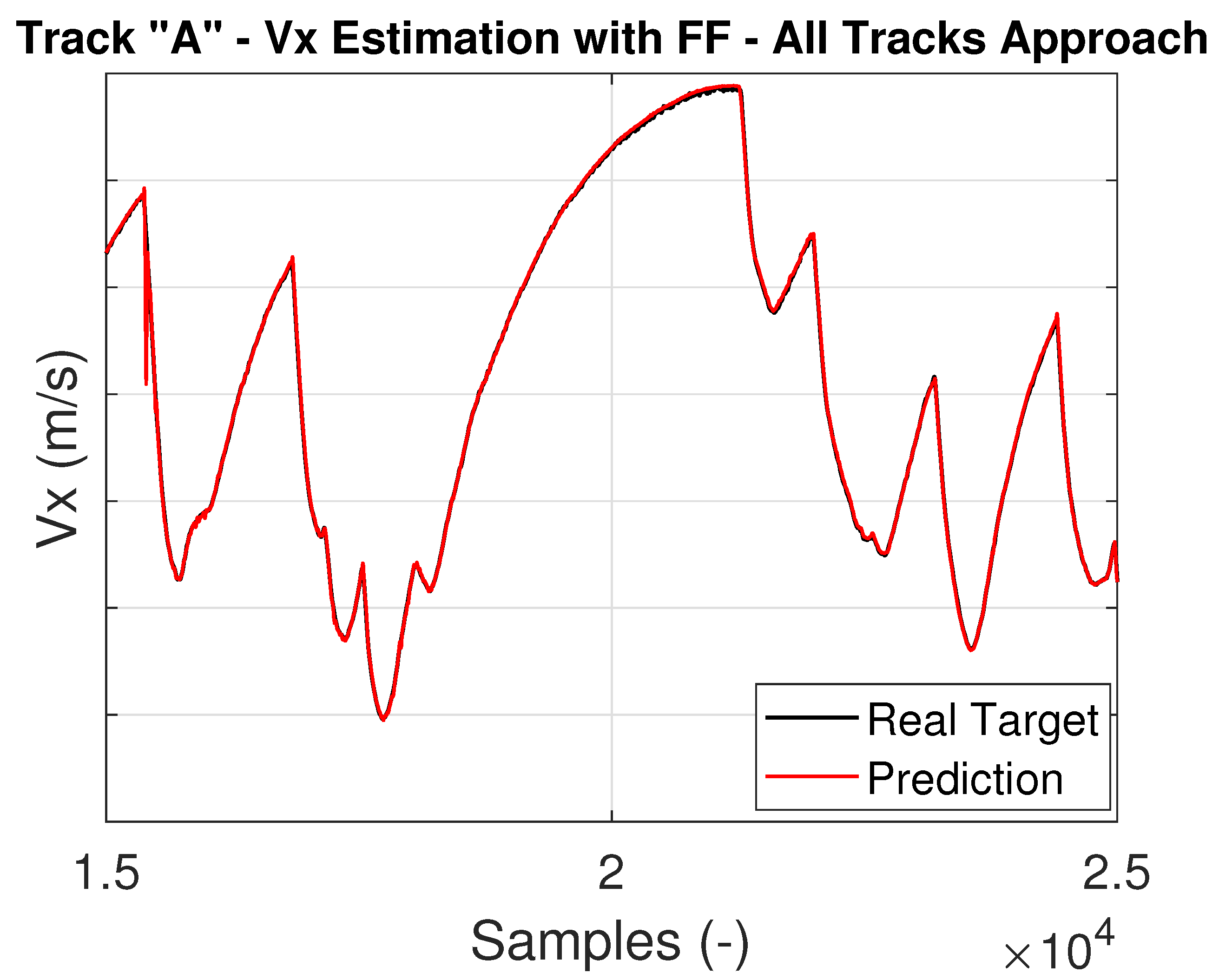
42]. In more detail, the proposed methodology introduces a dual-network architecture, that is, two distinct neural networks working in sequence: one is a dedicated neural network for estimating the longitudinal velocity, while the other is a separate neural network for predicting the sideslip angle, which also takes as input the longitudinal velocity estimate made by the previous network. In this way, after training the two networks appropriately, it is possible to create a virtual sensor that can replace the optical one. This virtual sensor estimates the longitudinal velocity of a vehicle using commonly found sensors. Then, a second neural network can be fed with this velocity and data from the same sensors to obtain an estimated sideslip angle at any given time. By implementing the trained networks on the vehicle control unit, these estimates can provide real-time information that improves the operation of driver assistance systems, without requiring expensive sensors. It can also help improve the vehicle’s dynamic behavior and performance where necessary.
The paper presents, in
Section 2, a brief overview of the sensors installed on the vehicle, of the acquired channels, and of the tests performed with the aim of deepening the capability of the neural network;
Section 3 presents the types of neural networks used and how they were designed. In
Section 4, the data preparation procedure is presented; this is a critical aspect for a machine learning model to work properly. Finally, in the last section, a detailed comparison of the results related to the different types of trained networks is reported, with particular attention to the key performance indicators (KPIs), which is useful to define the best solution for the presented case study.
2. Sensors and Test Methods
In the context of this research activity based on an artificial neural network, where inputs rely on specific values acquired through sensor data, it is necessary to present a comprehensive overview of the sensor technologies used to collect the necessary data for feeding the artificial neural network (ANN). This paper focuses on various analyses for sideslip angle estimation using a high-performance reference vehicle equipped with multiple sensors placed in various locations to gather data for the ANN. Additionally, key characteristics of the reference vehicle, such as the center of gravity (CoG) position, tire specifications, and engine and suspension features, were also known. Acquisitions were made on different circuits that had varying characteristics and layouts. One of them was identified by tight, slow turns that had a high aerodynamic load. The other one had the opposite characteristics, with long straights and a low aerodynamic load. The third circuit had intermediate characteristics, with several fast corners. On all these circuits, the vehicle was sensorized in the same way. In addition, with the same tires and on each circuit, long runs and short runs were performed with the same vehicle. In the former, the driver was more focused on tire management and had more fuel load; in the latter, the driver was more focused on performance. In addition, limit situations such as tire locking under braking were also tested so that the NN could also be trained to recognize particular phenomena with different slip values.
The data acquired from the sensors are often subject to noise, electromagnetic disturbances, and high-frequency vibrations. Therefore, a preliminary operation involved filtering the channels of interest to remove the noise from the acquired signals. Considering unavoidable misalignments between the sensors and the vehicle’s reference system, it was essential to detect and eliminate these offsets. Additionally, to compare the outputs from various instruments mounted in different parts of the vehicle, all of the data were reported to the center of gravity (CoG).
2.1. Input Channels
This research activity, as previously mentioned, aims to estimate the sideslip (
) angle through the use of neural networks (NN). The input channels for the NN, which are useful to achieve the mentioned evaluation, are presented in
Table 1.
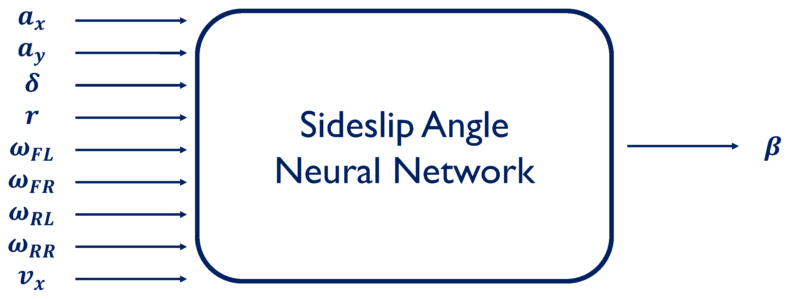
A block diagram that summarizes the structure of the neural network inputs is depicted in
Figure 1.
These channels are essential in the field of vehicle dynamics, as they are useful to describe the vehicle’s behavior during both cornering and straight-line driving. For this reason, these variables were chosen as inputs for the neural network to estimate the sideslip angle.
In addition, to acquire data in different conditions, several analyses were performed by varying both the road and the tire conditions. Indeed, in this way, it was possible to understand the influence of these variables on the sideslip angle estimation.
2.2. Equipped Sensors
The input channels for the neural network are obtained from various sensors properly mounted on the reference vehicle. For what concerns the steering angle and the wheels’ speed of the four corners, these are acquired from the vehicle CAN-bus [
43]. A controller area network (CAN-bus) is a standardized vehicle communication network, developed to facilitate communication between microcontrollers and a variety of sensors, all without the dependency on a central host computer [
44,
45]. It employs a message-based protocol consisting of four frame types: Data, Remote, Error, and Overload. The Data frame is the only one for actual data transmission. Each device transmits data serially, and if multiple devices attempt to transmit simultaneously, the highest priority device continues while others yield. The CAN-bus is then essential because it enables communication among the various instruments mounted on the vehicle for data acquisition and provides crucial data for this research activity.
Differently, the acquisition of the yaw rate and both lateral and longitudinal accelerations is achieved with an inertial platform (depicted in
Figure 2a). A sensor module comprising three accelerometers and three gyroscope units, functioning as angular rate sensors, is employed to calculate all resultant outputs. It is based on mathematical algorithms used to make precise real-time measurements of motion. Utilizing the Global Navigation Satellite System (GNSS), the instrument has the capacity to rectify all recorded parameters, thereby ensuring the accurate assessment of metrics such as accelerations, roll, pitch, and yaw. All of the data are processed in real time, time-stamped, and synchronized with GPS time. This information is transmitted over the CAN-bus and can be viewed in real time on a laptop using specialized software.
To determine the longitudinal velocity and the reference sideslip angle for training the artificial neural network, an optical sensor is employed (depicted in
Figure 2b). This instrument, utilizing Correvit technology, is valuable for directly measuring vehicle velocity and its components through non-contact measurements. A built-in GPS receiver enables the acquisition of position and speed data, while integrated accelerometers allow for the detection of the vehicle’s longitudinal and transverse accelerations. Additionally, integrated angular rate sensors measure pitch and roll angles, as well as the rotation around the vehicle’s vertical axis. Furthermore, the sensor also calculates additional signals such as leveled acceleration and curve radius.
A schematic representation that summarizes the associated instruments for the various neural network inputs is presented in
Table 2.
The described sensors are all linked through an external data acquisition system with the ability to collect a range of signal types and ensure their proper synchronization.
In the motorsport field, the use of optical sensors on vehicles during races and official test sessions is constrained by specific regulations. This restriction leads to less information that is useful to improve the overall vehicle performance. Additionally, it is essential to note that the sensors presented are both expensive and delicate, making them impractical for installation on all vehicles.
Hence, the proposed methodology, which relies on neural networks for estimating the sideslip angle, offers an effective solution for overcoming the challenges associated with sensor equipment. In particular, with regard to the input related to longitudinal velocity, this paper presents two cases: the first case uses the value from the optical sensor as input, while the second case employs the estimation of longitudinal velocity based on the procedure presented in [
42]. The novelty of the proposed methodology lies precisely in this second approach, that is, the introduction of a dual-network architecture, consisting of a dedicated neural network for longitudinal velocity estimation and a separate neural network designed for sideslip angle prediction, which is also fed with the estimated longitudinal velocity. So, this innovative approach involves the collaboration of two distinct neural networks operating in cascade, each addressing specific aspects of the system dynamics. In this way, it is possible to design a virtual sensor that replaces the optical one.
3. Artificial Neural Networks
Deep learning is a groundbreaking technology in artificial intelligence. It uses artificial neural networks to recognize patterns and make intelligent decisions, revolutionizing how we tackle complex problems and interpret large datasets.
An artificial neural network, a construct of interconnected neurons organized into layers, operates as an adaptable system. This adaptability allows it to modify its internal structure by assimilating information during the training phase, fostering its ability to process and analyze data effectively [
46]. This network can simulate complex relationships between inputs and outputs, which can be challenging for traditional analytic functions. Moreover, neural networks can generalize their learning, accurately generating outputs for inputs not in their training dataset through multiple learning cycles [
47]. It is precisely this remarkable ability to adapt and generalize that piques our interest in this work [
48].
3.1. Artificial Neural Network Structure
To properly understand how the developed model to evaluate the sideslip angle works, it is necessary to deep into the most important features of an artificial net. Every neuron in a neural network has multiple inputs that can be either the input signals of the problem or signals coming from previous neurons (
Figure 3). These inputs are added up for each neuron based on the weight of their connections. During the training phase, the weights are adjusted to enhance the overall learning of the network. Additionally, every neuron in the network has a bias that helps in fine-tuning the optimal working point of the neuron. Another crucial aspect of the neuron is the activation function that determines its output based on the inputs, weights of the connections, and the bias. In brief, the neuron’s ability to learn and adapt is governed by these key features.
Hence, the output of a neuron is returned by Equation (
1).
where
are the weights of the i-th neuron;
are the inputs of the i-th neuron;
is the bias of the i-th neuron;
is the output of the of the i-th neuron;
f is the activation function.
As mentioned, multiple neurons aggregate to create neural networks, complex structures organized into layers. These layers include an input layer, an output layer, and one or more intermediate layers, which are called hidden layers. The number of hidden layers and neurons in each layer varies based on specific application needs, with no fixed rules dictating their selection.
3.2. Artificial Neural Network Training
Training a neural network involves optimizing the weights and biases associated with its neurons, specifically for a subset of the dataset known as the training set. The goal is to progressively minimize prediction errors. To achieve this, an error or loss function, along with an algorithm, is introduced. The backpropagation algorithm, which is based on gradient descent methods, is commonly used to reduce the error between the network’s output and the desired target.
In essence, after a forward pass, backpropagation adjusts parameters through a backward pass, fine-tuning the model [
49]. It starts with random weight and bias initialization, comparing results to target outcomes, leading to the loss error function. The gradient descent method then calculates partial derivatives to identify influential nodes in minimizing loss, as shown in Equation (
2).
where
represents the updated weight (or bias) at time .
represents the current weight (or bias) at time t.
is the learning rate, which controls the step size for weight updates.
Those nodes receive smaller weights to reduce the overall loss of the model. In other words, it measures how sensitive the loss is to changes in each weight. This is carried out using calculus and gradients to determine the direction and magnitude of the steepest increase in the loss. The learning rate controls the update magnitude, with smaller rates leading to more stable convergence, but more iterations may be required. Larger rates can speed up convergence but risk overshooting the minimum. In summary, during each training cycle (epoch) of the neural network, the backpropagation algorithm adjusts weights by subtracting derivatives scaled by a “learning rate” (which avoids abrupt variations of the weights). This iterative optimization process continues until the error function reaches a desirable threshold for the application.
To perform the explained training process of the neural network, the authors decided to use the Levenberg–Marquardt algorithm. From the foundational principles of standard backpropagation with gradient descent, the Levenberg–Marquardt algorithm emerged as an innovative optimization method for neural network training. This algorithm introduces a novel approach by incorporating the Hessian matrix, capturing the second-order partial derivatives of the cost function with respect to network weights. It dynamically adjusts a damping parameter to modulate the step size in weight updates, adapting to the local curvature of the cost function’s surface. The resulting weight updates become a function of the gradient, Jacobian matrix, error vector, and Hessian matrix, enabling faster convergence and improved stability during training. Its functioning is summarized in Equation (
3).
where
represents the updated weight (or bias) at time .
represents the current weight (or bias) at time t.
J is the Jacobian matrix, representing the first-order partial derivatives of the cost function with respect to the weights.
e is the error vector, representing the difference between the network’s predictions and the target values.
represents the diagonal elements of the Hessian matrix.
This method is particularly valuable when training neural networks with relatively few weights and is recognized for its ability to expedite the optimization process in various scientific and engineering domains.
3.3. Overfitting Phenomenon
A recurring problem when using supervised learning models is the occurrence of overfitting. Overfitting is a common challenge in machine learning where a model is trained to learn from a specific dataset to the point that it becomes too specialized to that dataset. This can lead to the model becoming less accurate, or even ineffective, when presented with new, unseen data. Essentially, overfitting occurs when the model has learned to recognize the training dataset so well that it becomes unable to generalize and make accurate predictions on new data. For this reason, a validation procedure is necessary to prevent the occurrence of the overfitting phenomenon. There are several ways of performing the validation process that can be grouped into two categories:
Dataset split or data partitioning: This allows for the evaluation of the model’s performance on a separate set of data that the model has never seen before;
Cross-validation: This involves dividing the dataset into multiple subsets (folds) and systematically training and testing the model on different combinations of these folds to assess its generalization performance and to tune hyperparameters.
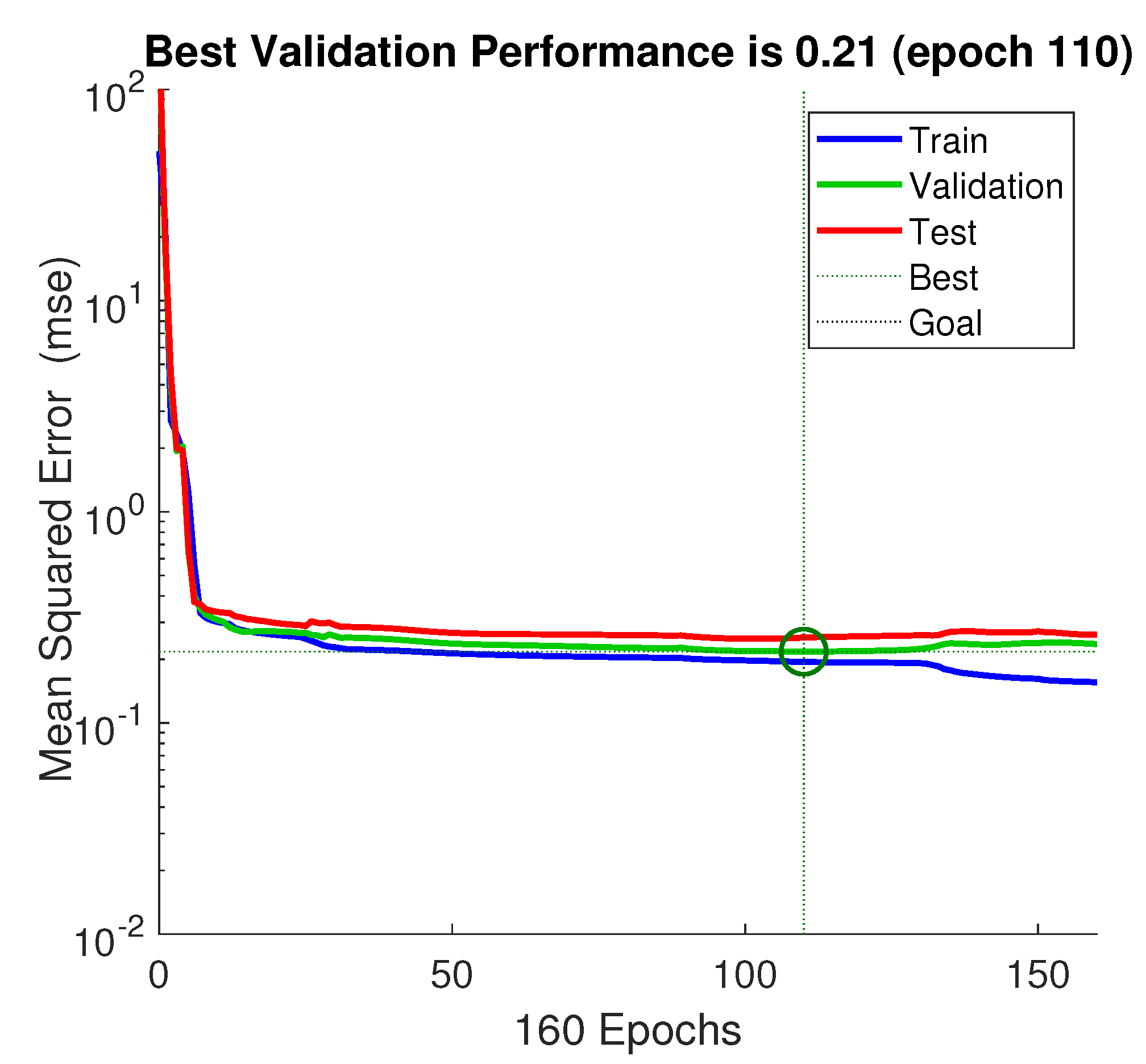
In this work, it was decided to use the data-partitioning technique to avoid overfitting. This decision was made because a relatively large dataset was available, so dividing it did not pose any risk to net training. With this technique, the overall dataset is divided into two subsets: a training subset and a validation subset. The former is used to train the model, while the latter is used to verify that the model generalizes correctly. Specifically, if the model’s performance on the validation set starts to degrade while the training error continues to decrease, it is possible to stop the training to prevent overfitting.
Furthermore, in order to utilize the extensive dataset effectively, a test subset was included for independent evaluation at the end of training. This subset helps to assess the model’s performance on unseen data, providing an unbiased estimate.
Regarding this division of the dataset, it was performed on Matlab with the appropriate “Divideblock” function, with which data are split into three subsets using three contiguous blocks of the original dataset. The fraction of the original data that goes into each subset is as follows:
of the dataset for the training phase;
of the dataset for the validation phase;
of the dataset for the test phase.
The dataset was divided in this way strategically to strike a balance between preventing underfitting, ensuring an adequate number of training samples, and guarding against overfitting by providing a sufficiently sized validation set for assessing model generalization.
3.4. Neural Network Architectures
This section describes the neural network architecture typologies used in this study. Indeed, there are different types of neural networks whose choice depends on the application and complexity of the problem to be solved. As the research deals with discrete-time sequences, two types of networks were considered for the study:
Feedforward neural networks (FNNs) follow a structure where connections exclusively link neurons from one level to the next. These networks lack backward connections or links between neurons at the same level. This architecture means that FNNs do not retain a memory of past events, and their output solely depends on the current inputs [
50];
Recurrent neural networks (RNNs) are a class of neural networks characterized by the presence of loops: the output values of a higher-level neuron (closer to the output) can be used as an input for a lower-level neuron (closer to the entrance). Thanks to the looping mechanism, RNNs have an internal memory [
51].
More in detail, as for recurrent neural networks, two different variants of them have been tried and compared:
3.5. Neural Network Hyperparameters
This section presents the neural network hyperparameters chosen for the study, including the number of neurons, hidden layers, epochs, and learning rate value. It is crucial to set these parameters accurately to avoid overfitting, underfitting, and lack of prediction accuracy.
The selection of the number and dimensions of
hidden layers is motivated by the problem’s intricacy. Since the very complex trend of the sideslip angle time series, a neural network architecture with two hidden layers is employed in this work. Indeed, networks with two hidden layers are capable of representing functions of any shape and complexity, while, based on current understanding, there is no theoretical justification for using neural networks with more than two hidden layers [
54]. The use of two hidden layers offers increased modeling capacity while managing computational resources effectively. This configuration strikes a balance between complexity and training efficiency.
There are many rule-of-thumb methods for determining the correct number of neurons to use in the first hidden layers. Choosing too few neurons can result in underfitting and high statistical bias. On the other hand, selecting too many neurons can lead to overfitting, high variance, and a longer training time. To achieve a balance between accuracy, generalization, and processing time, the following guidelines were followed:
Starting from these observations, the number of neurons in the first hidden layer was set to the size of the input layer plus one for the output layer size. Regarding the number of neurons in the second hidden layer, a looping mechanism was introduced to systematically explore various combinations of neurons in both hidden layers. The goal was to optimize the network’s performance through multiple training sessions driven by the looping mechanism. Subsequently, the network configuration with the pair of neurons that minimized a specific error function was selected. The neural network with the optimal pair of neurons was subjected to additional training to assess if further performance improvement was achievable. If the performance showed positive enhancement during this additional training, the last trained network was retained. Otherwise, the previous configuration was reinstated. Ultimately, the best-performing neural network configuration, as determined by this process, was used for making predictions.
Neuron initial weights are not defined because the correlation between input and output is not preventively known, so they were defined randomly by software.
The number of epochs, that is, the number of presentations to the network of all patterns in the training set, was chosen equal to 200 to find the best trade-off between the quality of results and the network processing time. Once the epochs were chosen, the number of validation checks for early stopping was set too. Early stopping is a regularization technique where training is halted when the validation performance no longer improves, preventing overfitting. This value was set equal to the of the number of epochs.
The choice of activation functions influences the network’s ability to capture nonlinearities in the data. For the type of data linked to this application, the hyperbolic tangent (tanh) activation function was chosen. This function maps input values to a range , and is commonly used in neural networks for its ability to model nonlinear relationships.
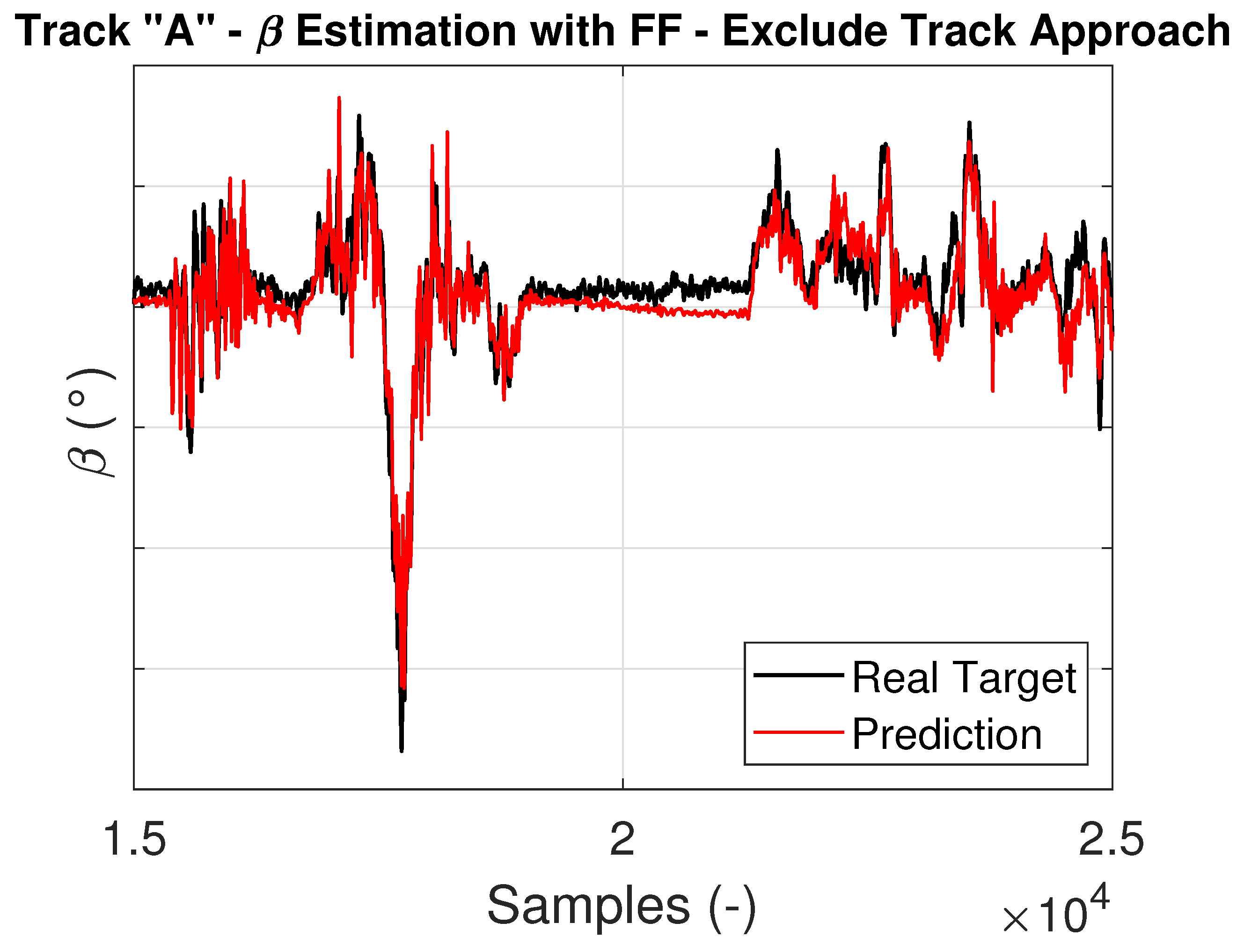
Finally, it is important to underline that the networks have been trained with different dataset configurations to evaluate the effect on the estimation accuracy and the possible occurrence of overfitting. In more detail, the nets have been trained using both a dataset with all circuits and one without the circuit on which the prediction was then made. In addition, the prediction was made considering both new and worn tires.
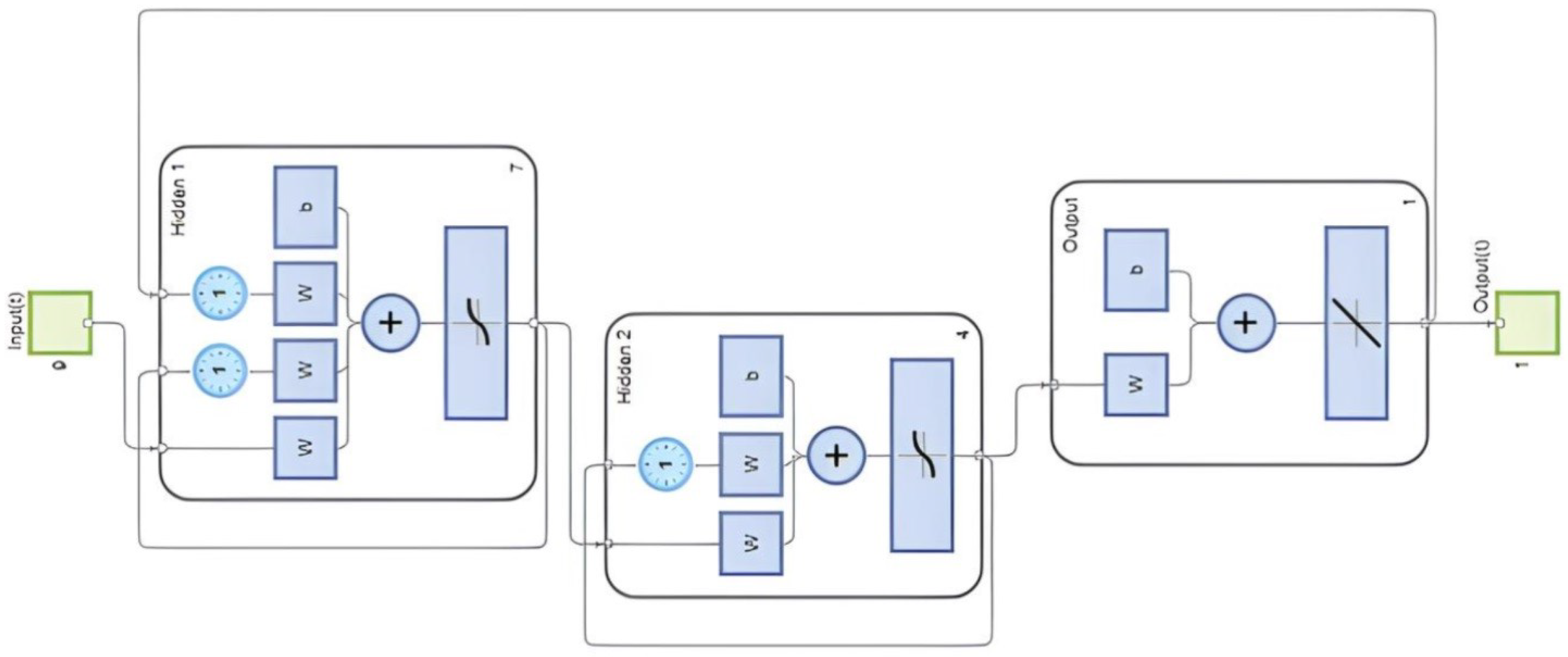
These settings were used for all designed neural networks, and they are summarized in
Table 3 and shown in
Figure 4,
Figure 5 and
Figure 6, where the schemes of these nets are reported.
3.6. Model Evaluation
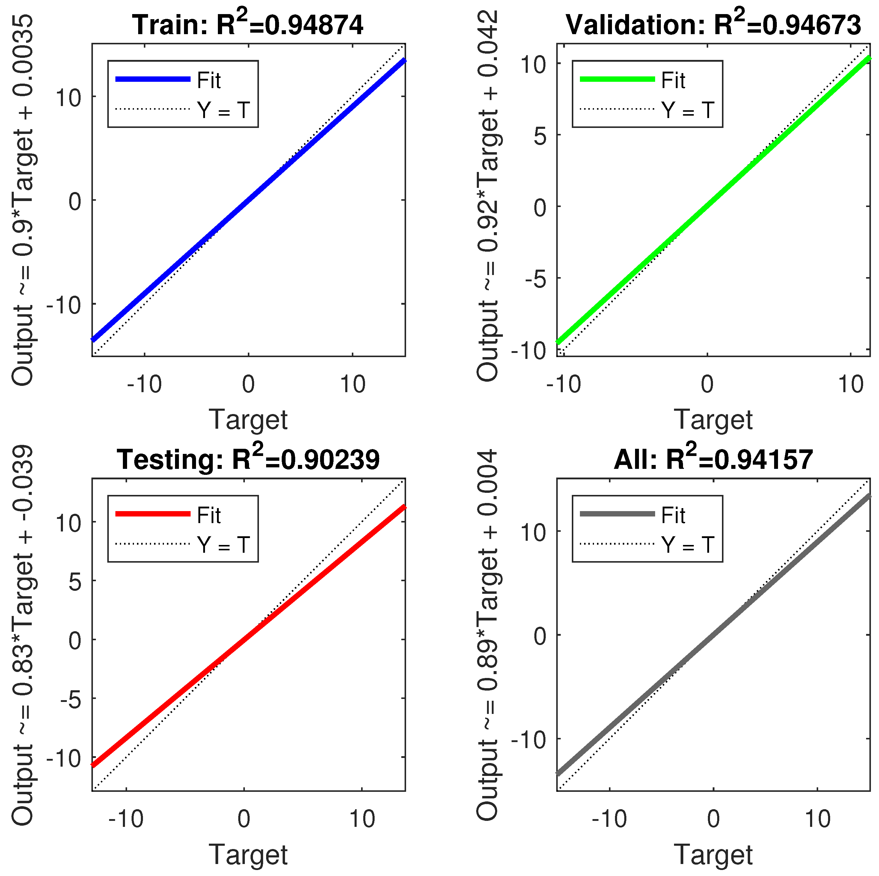
To evaluate the performance of the neural network in terms of estimation error, the root mean square error (RMSE) is employed. This is a widely used metric for assessing the accuracy of a prediction model, usually in regression analysis. It considers the magnitude of the error between the predicted values and the actual values. Together with the RMSE, with the same aim, it is used also the coefficient of determination. It is a statistical metric used to evaluate the goodness of fit of a regression model. It measures the proportion of the variance in the dependent variable (the target) that is explained by the independent variables (predictors) in the model. It results in a value between 0 and 1, where a higher value indicates a better fit of the model to the data.
3.7. Analyzed Approaches
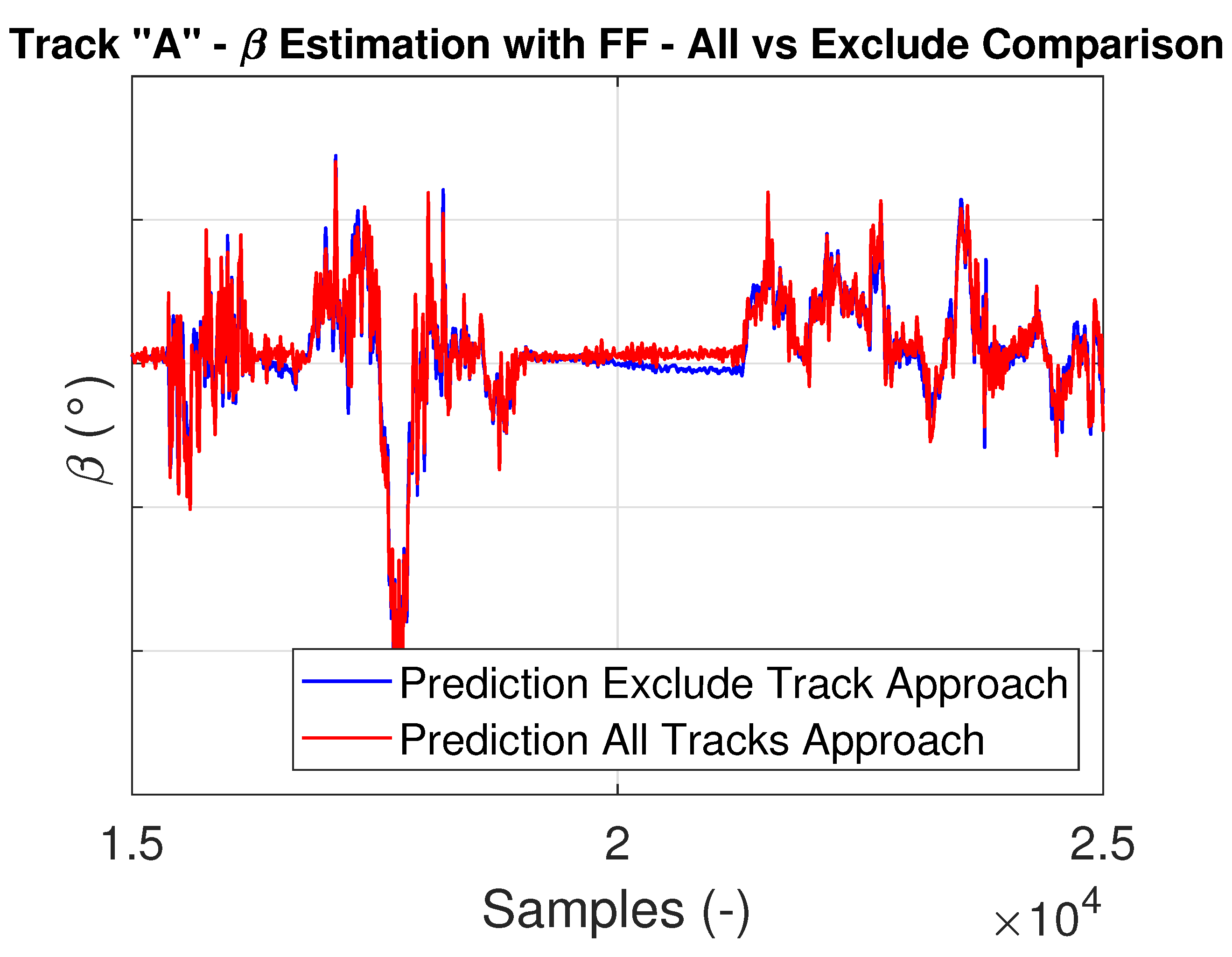
In this part, an explanation of the approaches, which are aimed at enhancing the accuracy of the angle prediction performed by the network and the ability to generalize correctly of the network itself, is presented. For what concerns the ability of the network to work with circuits having different layouts—and therefore, characteristics—the following approaches have been tried:
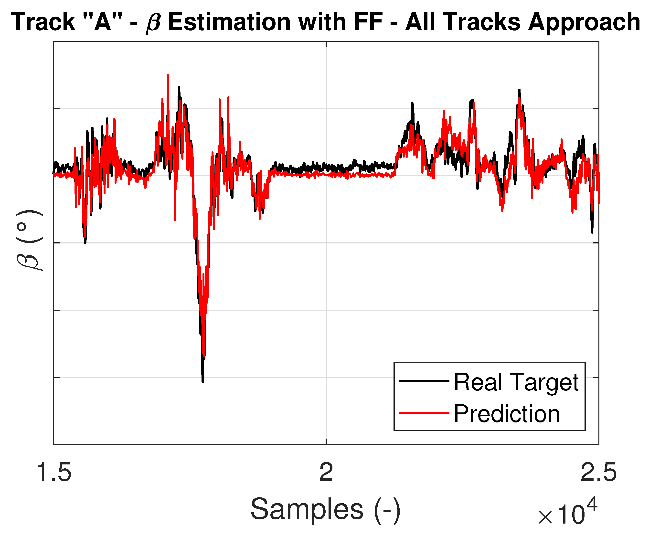
All Tracks: For training and validating the neural network, data from all the available tracks are used. The system randomly selects data for the training set and uses the remainder for the validation and test subsets;
Exclude Track: The neural network is trained on a dataset from which all data related to a specific track have been removed. These data are then used for the prediction and performance evaluation of the net.
Additionally, the model has been verified to predict the sideslip angle on the same track, using tires with varying levels of wear, thus demonstrating its adaptability to different tire wear levels [
20].
4. Data Preparation for Neural Networks
In the machine learning world, data preparation is an important first step in transforming raw data into well-structured data, optimized for successful use in machine learning models; indeed, the overall performance of these models is highly dependent on the quality of data preparation performed. Great care and attention to this important process are therefore necessary to achieve the best results. Data preparation includes methods such as data cleaning and filtering, data normalization, feature engineering and selection, handling of missing values, dimensionality reduction, and so on. The quality of data preparation plays a significant role in the accuracy and efficiency of a machine learning model. The main goals pursued in this step for the model under consideration were as follows:
Improved model accuracy: Data preparation enhances the quality of the dataset, leading to more accurate and reliable machine learning models;
Enhanced feature relevance: data preparation allows for effective feature selection. By selecting the most informative variables, the model can make accurate predictions while reducing the risk of overfitting. This, in turn, ensures that the model can generalize well and avoid loss of accuracy;
A faster and more efficient training phase: Well-prepared data speed up model training, reducing computational burden and processing time.
4.1. Data Cleaning
The first steps taken to prepare the dataset were the following basic data-cleaning operations are as follows:
These steps are essential to prepare the dataset for the model. They ensure that the data are in a format that is compatible with the model, and that it does not contain any useless information that may impair its operation.
4.2. Feature Selection
The process of feature selection involves reducing the number of input variables used in a model to only the most relevant ones. In this context, relevance refers to the link between the input quantities and the target used for training. This procedure has three main aims:
By retaining key features and eliminating irrelevant ones, it boosts a model’s predictive performance;
It guards against overfitting by reducing data complexity and focusing on crucial attributes;
Models with fewer features are quicker to train and less resource-intensive, which ia ideal for large datasets and real-time applications, reducing computational costs.
In order to select the features for the neural network responsible for predicting sideslip angle, a methodology was employed that combined concepts and equations of vehicle dynamics [
16] with the channels that can be obtained through sensors that are easily installed, purchased, and used on various types of vehicles, as explained in
Section 2. Using this information, the most relevant acquired channels were selected.
4.3. Data Filtering
As stated in
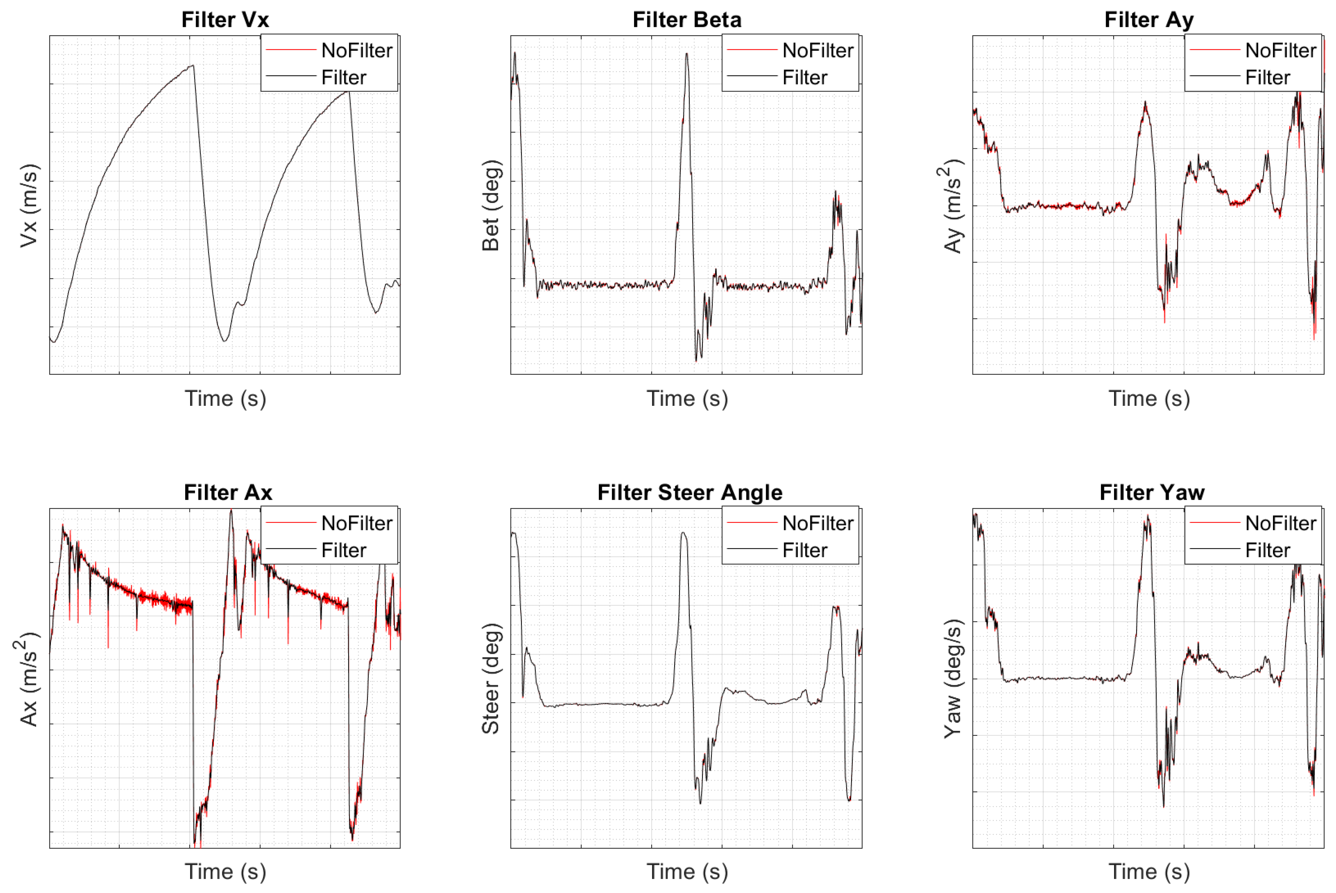
Section 2, acquired data need a preliminary filtering operation. Signals acquired from various sensors in a vehicle are subjected to different types of noise, such as electromagnetic interference, sensor inaccuracies, and environmental factors, so the information they provide to the tool could be not directly linked with the phenomena involved in the vehicle dynamics field. Filtering becomes crucial in reducing this noise to ensure that the data obtained are more reliable and accurate. For this purpose, a Butterworth filter is used, which is a type of signal-processing filter designed to have a frequency response that is as flat as possible in the passband. In particular, a third-order, 5 Hz low-pass filter is used, with a Nyquist normalizing frequency depending on the sampling rate, commonly equal to 50 or 100 Hz. The results of the filtering operation can be seen for all the channels of interest in
Figure 7.
4.4. Static and Dynamic Offset Detection
On-board instrumentation in vehicles is often installed with misalignments between its own reference system and that of the vehicle. This can lead to miscalculations during certain procedures. To prevent this, it is important to detect and correct these misalignments or offsets. There are two types of offsets that can be identified: static and dynamic. To fix these offsets, the authors followed the subsequent procedures:
In order to detect the static offset, it is required to select a range of data acquisitions with the vehicle in stationary conditions. Once the range is selected, the average values of longitudinal and lateral accelerations, as well as longitudinal velocity channels are calculated within the selected range. These average values are then subtracted from the original signals;
To detect the dynamic offset, a specific range of acquisitions is chosen in which the vehicle is moving on a straight line with a constant speed, usually in the pit lane. Once the range is selected, the average steering angle, yaw rate, and sideslip angle values are calculated within that range. These average values are then subtracted from the original signals to obtain the dynamic offset.
The non-contact optical sensor, which was used to acquire longitudinal velocity and sideslip angle, can have also an inclination in the
plane. This inclination can be calculated with Equation (
4).
where
and
are, respectively, the mean of the longitudinal and lateral velocity measured in straight stationary maneuvers. This angle enables the correction of optical sensor measurements.
4.5. Outliers Removal
A technique based on median absolute deviation (MAD) was used for identifying and dealing with outliers in the dataset. MAD is a robust statistical measure, based on calculating the distance between the median of each point in the univariate distribution (single channel in the dataset) and the median of the distribution itself, as described in Equation (
5).
Instead of using the mean and standard deviation (standard z-score method for outliers imputation), this method uses the median as the measure of central tendency and the median absolute deviation to quantify the spread or dispersion of the data, as can be seen in Equation (
6). The median is robust to outliers and represents the center of the data without being heavily influenced by extreme values. The MAD is also robust to outliers and characterizes the variability in the data without being distorted by extreme values [
55].
where if
, then
is considered an outlier. The threshold value, as in the standard z-score method, is chosen according to the application.
In summary, the MAD-based z-score method was preferred over the standard z-score for identifying and handling outliers because it is less influenced by extreme values, interpretable, and robust in various data scenarios.
4.6. Data Standardization and Transformation
Input and output variables involved in the data acquisition process are, generally, physical quantities of different types. For this reason, they may have very different magnitudes, which could affect the artificial neural network negatively. When the data used for training a network have significantly different magnitudes, the convergence and learning process can be slowed down significantly. In some cases, this can cause the network to not effectively perform the learning process [
56]. This is why the quantities of interest for the model should be preprocessed in order to obtain magnitudes all within the same range. Normalization and standardization are two widely used preprocessing methods to achieve that. In this paper, a process of standardization has been performed. This process, for each predictor individually, involves scaling data so that the mean results in zero (centering), and the standard deviation results in unity and retains the shape properties of the original dataset, that is, the same skewness and kurtosis [
57].
The standardization related to a generic observation
is defined as in Equation (
7).
where
is the mean, and can be defined as in Equation (
8), and
is the standard deviation, and is defined in Equation (
9).
It is crucial to emphasize that to prevent data leakage, the process of standardization should only be performed on the training subset. Afterward, the same values of mean and standard deviation should be used to standardize the channels associated with the validation and test subsets.
6. Conclusions
A novel method for estimating vehicle sideslip angles using a neural network-based approach has been introduced. The outcomes of this research consist of a machine learning model where the inputs are typical vehicle dynamic signals: steering angle, lateral and longitudinal acceleration, yaw rate, and wheel speeds. These signals are accessible from the CAN-bus, as they are commonly measured in both motorsport and passenger vehicles.
The analysis was conducted using various neural network architectures. This phase aimed to understand which net design, between feedforward, NARX, and recurrent neural networks, was more suitable for the prediction of the quantity of interest. The results showed that feedforward and NARX give very similar results but feedforward, having no feedback, is much faster. The worst was the recurrent neural network, both for accuracy and training time. These results arise because the feedback signal cannot exhibit significant delays to maintain real-time operational conditions and because the inaccuracies present in some parts of the estimate negatively interfere when going as input by means of the looping mechanism.
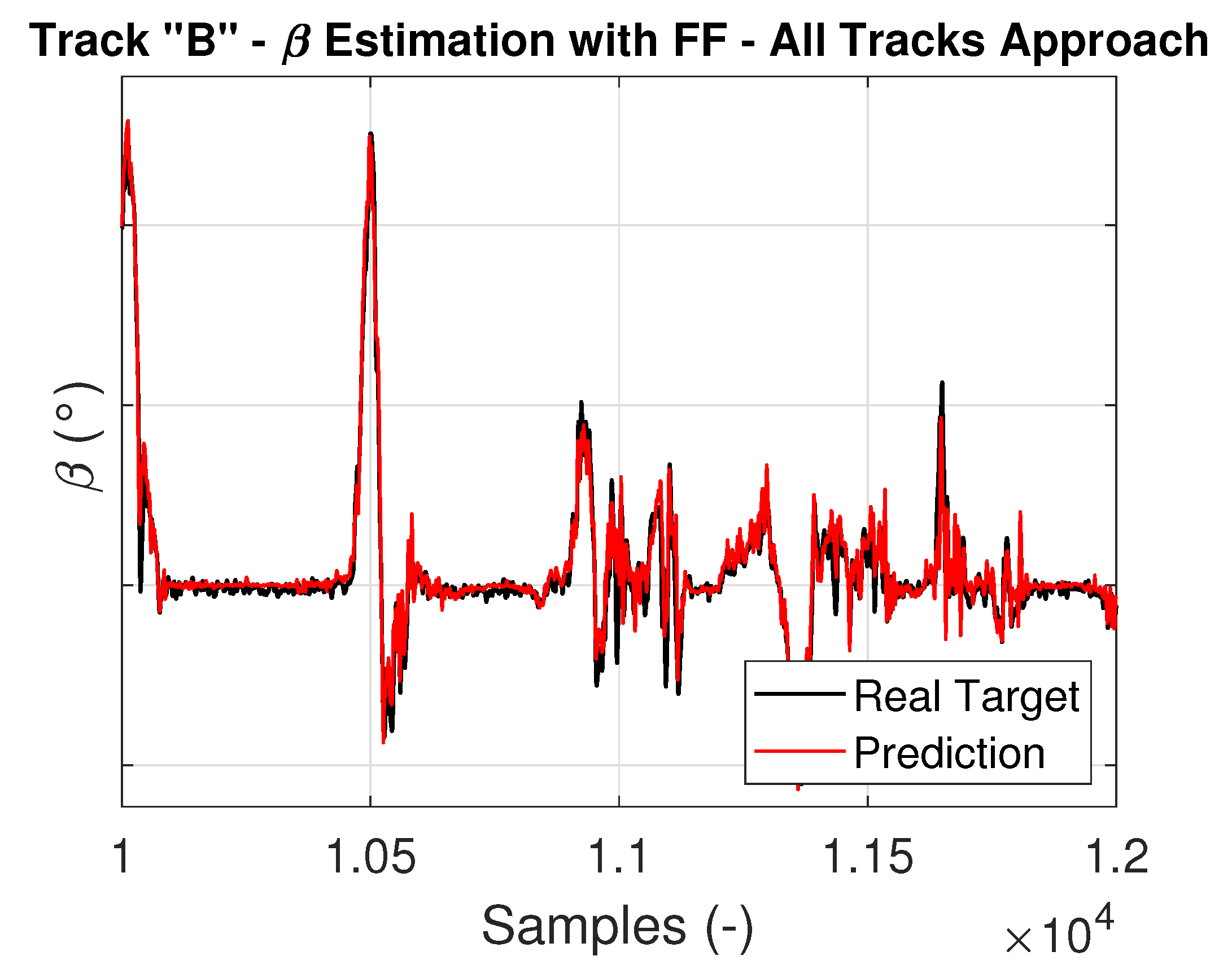
The network’s generalization capability was thoroughly tested across various scenarios, including multiple runs on different tracks while taking into account both new and worn tires. This testing approach aimed to assess the model’s adaptability and robustness under various real-world conditions. By examining the network results on various circuits, each with unique characteristics, its ability to make accurate predictions across different track configurations was evaluated. The network demonstrated its ability to consistently estimate the angle of interest across different scenarios, showcasing its adaptability and suitability for various applications. Furthermore, the network was tested on both new and worn tires to account for variations in tire conditions, evaluating the model’s solidity to changing tire properties throughout its life cycle. The results highlighted the network’s remarkable capability to maintain accuracy and reliability, regardless of the tire’s structural and viscoelastic properties, further underlining its real-world applicability. The neural network’s great generalization performance across various circuits and tire conditions reinforces its potential for onboard applications, where it can provide real-time estimations of vehicle dynamics quantities with consistently high precision and reliability. For this purpose, the accurate results obtained by it when cascaded by another neural network that estimates longitudinal velocity are crucial.
The methodology utilized in this study presents several important advantages, with one of the most prominent being its ability to provide accurate, near-instantaneous, real-time estimations of this fundamental physical quantity. The strong agreement between the estimated sideslip angle and the acquired one supports the suitability of these procedures for onboard implementation, rendering the need for bulky and expensive instrumentation obsolete. In summary, the machine learning model utilized in this study has low computational requirements and provides reliable outcomes, making it ideal for use in onboard control systems, such as ABS and TCS.
In order to further enhance the benefits of the presented model, our next steps involve utilizing its outputs to feed vehicle dynamics models that can accurately calculate the slip and forces applied to the tire. These models will integrate with the driver assistance systems to further improve their precision so as to increase safety and performance. However, before implementing this, we plan to thoroughly test the model’s functionality on various types of vehicles, in order to expand its use.
