An Improved Cuckoo Search Algorithm under Bottleneck-Degree-Based Search Guidance for Large-Scale Inter-Cell Scheduling Optimization

Abstract

In order to deal with problems of reduced searching efficiency and poor quality of algorithms for large-scale inter-cell scheduling problems, an improved cuckoo search algorithm under bottleneck-degree-based search guidance is proposed. A large-scale inter-cell scheduling optimization model aiming at minimizing makespan is established. A tabu search is adopted to replace the local search strategy of the cuckoo search algorithm. The bottleneck degree of a complex network model for an inter-cell scheduling problem is used to guide the design of the neighborhood structure of the tabu search. The proposed algorithm is validated by numerical examples. The results show that the convergent speed and qualities of solutions of the proposed algorithm are improved. It is verified that the proposed search guidance based on a complex network’s bottleneck degree could improve the searching ability and convergence speed of the algorithm for large-scale inter-cell scheduling optimization problems.

1. Introduction

Large-scale scheduling optimization problems have attracted much attention from both academia and industry. Scheduling problems involving more than 20 machines and 50 parts are defined as large-scale scheduling problems [1]. As manufacturing tasks and resources increase, the space of feasible solutions for an algorithm to solve large-scale scheduling problems increases exponentially. Finding an optimal solution within a reasonable computation time is challenging for most algorithms [2]. At the same time, diversification and personalization of products receive attention, resulting in the need for manufacturing enterprises to quickly meet the market demand for variety and small batches. Inter-cell scheduling has gradually become an essential method for sharing resources in manufacturing. Inter-cell scheduling problems involve intra-cell scheduling optimization and inter-cell scheduling optimization of exceptional parts, which is more complicated than job-shop scheduling problems [3]. Therefore, it is necessary for algorithms to have high searching capability to solve large-scale inter-cell scheduling problems.

There are two common ways to solve large-scale scheduling optimization problems. One is to decompose large-scale scheduling problems into several sub-problems, based on decomposition strategies [4]. According to decomposition mode, methods to decompose a large-scale scheduling problem can be classified into time-oriented, machine-oriented, and job-oriented decomposition methods, etc. The time-oriented decomposition method is to divide a large-scale scheduling problem into several sub-problems by segmenting the total scheduling time into multiple time intervals. For example, refs. [5,6] divided the total time of a scheduling problem into several time windows and each sub-problem within a time window was optimized independently. However, the time-oriented decomposition method is difficult to apply for problems with unclear time segments. It is concluded that decomposition methods often rely too heavily on model constraints and decomposition modes. Other researchers [7,8] have proposed machine-based decomposition methods to reduce the complexities of solving large-scale scheduling problems. Machines were divided into several cells based on process similarity or constraints. Each cell was scheduled individually. However, exceptional parts in inter-cell scheduling problems require transportation to other cells, which makes sub-problems interconnected. The machine-oriented decomposition method has difficulty solving inter-cell scheduling problems. The job-oriented decomposition method is to divide jobs into several batches based on certain properties (e.g., due date of jobs) and schedule them independently [9,10]. It reduces the complexities of scheduling problems by reducing the number of jobs to be scheduled. Key issues for the method include job combination and batch size, which require a deep understanding of the problems [11]. In addition, not only the job-oriented decomposition method but also all the decomposition methods mentioned above find it difficult to yield global optimal solutions for original large-scale problems due to focusing on scheduling sub-problems [12]. Although these decomposition methods can simplify large-scale scheduling optimization problems, there are still some limitations and problems in real applications.

Another way to solve large-scale scheduling problems is to improve intelligent optimization algorithms. As spaces of feasible solutions and computational complexity increase exponentially with the scale of scheduling problems, it is difficult for intelligent optimization algorithms to yield acceptable solutions within a reasonable calculation time [13]. In order to solve large-scale scheduling problems, it is essential for intelligent optimization algorithms to improve their searching ability and convergence speed [14]. Efforts have been made using various methods to improve the performance of algorithms. One is introducing new mechanisms, such as opposition-based learning, designing new operators, setting adaptive parameters, etc. Cheng [15] introduced a pairwise competition mechanism to update particles in a particle swarm optimization algorithm (PSO) to improve convergence. The positions of particles that lost competitions were updated by learning from winners. Ali [16] designed a virtual crossover operator to improve the search ability of a genetic algorithm (GA). The parent chromosome was divided into several segments and offspring were obtained by exchanging segments based on certain rules. Qiao [17] designed an adaptive genetic algorithm to improve searching ability. Probabilities of crossover and mutation operations were dynamically adjusted according to population diversity. Other efforts have been made to design hybrid algorithms by combining strengths of two different algorithms. Algorithms with powerful local searching ability like tabu search (TS) and neighborhood search (NS) are often embedded into other intelligent optimization algorithms to enhance their searching ability [18]. Xie [19] proposed a hybrid algorithm that embedded TS into GA to improve searching ability. The proposed hybrid algorithm combined the excellent global searching ability of GA and powerful local searching ability of TS. Sun [20] proposed an improved hybrid genetic algorithm with variable neighborhood search (VNS) to solve flexible job-shop scheduling problems. A new neighborhood search to identify key processes on the critical path was designed to reduce the number of invalid transformations. Arindam [21] proposed a hybrid algorithm combining variable neighborhood search and cuckoo search (CS) algorithms. VNS was used to improve local search of CS to improve its overall search ability. The research mentioned above improved the searching ability and convergence of algorithms by complicating iterative processes. This means that it is difficult to guarantee the efficiency of algorithms for larger or more complex problems. It is necessary to explore other effective methods to improve algorithms for large-scale inter-cell scheduling problems.

Complex network theory is a powerful mathematical tool used to model and analyze complex systems [22,23]. It reveals properties and functions of various complex systems from interaction relationships and topological structure between elements of complex systems [24]. The theory has been applied to different types of complex systems, such as social networks [25], protein networks [26], public opinion networks [27], and transportation networks [28]. Complex network theory has been applied to the field of manufacturing scheduling in recent years. Becker [29] presented a multiple-attribute decision-making method to identify key machines in production systems. Production systems were modeled as complex networks in which machines were considered as nodes. Complex network features, such as node centrality, were used in the process of identifying key machines. Pang [30] proposed an improved ant colony algorithm based on a complex network model for a flexible job-shop scheduling problem (FJSP). The FJSP was abstracted into a complex network model. The path selection method and pheromone update rule of the ant colony algorithm were tailored to complex network structure and features. Zou [31] established a complex network model in which machines were considered as nodes for an inter-cell scheduling problem. An initial solution generation mechanism based on the modularity of the complex network was proposed to improve the convergence speed and solution quality of a small-world genetic algorithm. The above studies extracted complex network features that could reflect scheduling attributes in corresponding problems. These complex network features reflect features of scheduling problems. Analysis and utilization of these scheduling features has had guiding effects on the optimization of manufacturing scheduling. Therefore, exploring how to extract and use complex network features to guide the improvement of algorithms is a worthwhile research direction.

Large-scale inter-cell scheduling problems involve large numbers of interrelated manufacturing cells, resources, and tasks, which can be described and analyzed using complex network theory. Aiming at a large-scale inter-cell scheduling problem, a complex network model corresponding to a schedule was established. Complex network features related to scheduling including network efficiency, node load, betweenness centrality, and bottleneck degree were analyzed, and an improved cuckoo search algorithm under bottleneck-degree-based search guidance (TSCS-BD) is proposed. A tabu search has been adopted to replace the local search strategy in the cuckoo search algorithm. Bottleneck degree is used to guide the design of the neighborhood structure within the tabu search. In this study, complex network features are used to guide the algorithm search, which provides an effective solution for large-scale inter-cell scheduling problems.

2. Inter-Cell Scheduling Model Based on TSCS-BD

2.1. Problem Description

A large-scale inter-cell scheduling problem is an optimization problem and considers that n parts are scheduled to be processed on m machines located in u cells. Most parts can be processed in a designated cell, and there is no inter-cell move. Only exceptional parts need to be transported to other cells due to their manufacturing cell’s inability to meet the processing requirements for some of the processes. Additionally, some machines in different manufacturing cells have identical capacities. These exceptional parts have several candidate inter-cell processing routes, which is known as inter-cell manufacturing with flexible routes.

The problem considered in this paper is subject to the following assumptions:

(1)

All parts and machines are released at zero moment.

(2)

The processing route of a part consists of multiple operations that have sequence constraints.

(3)

For any operation, there is at most one machine in a cell that can process it.

(4)

Once an operation has started to be processed on a machine, it must not be interrupted until it is finished.

(5)

Operation of a job can be performed by only one machine at a time, and each machine can perform only one operation of any job at a time.

(6)

Exceptional parts are allowed to be transported to other cells and returned to the original manufacturing cell for subsequent processing.

(7)

Processing routes and processing time are known, and transportation time for parts in a cell is ignored.

(8)

Inter-cell transport capacity is adequate with no wait time.

2.2. Mathematical Model

2.2.1. Parameter Description

The following symbols are used for the problem formulation: definition of indices, sets, parameters, and decision variables, as shown in

Table 1. Symbol list.

Parameter	Parameter Meaning
$O_{\mathrm{ij}}$	The j-th operation of part i
$N$	Set of parts, N = {1, 2, ..., n}
$M$	Set of machines, M = {1, 2, ..., m}
$T_{\mathrm{ijm}}$	Processing time of operation $O_{\mathrm{ij}}$ on machine m
$S{T}_{\mathrm{ij}}$	Starting time of $O_{\mathrm{ij}}$
$C{T}_{\mathrm{ij}}$	Completion time of $O_{\mathrm{ij}}$
$T{D}_{\mathrm{mm}’}$	Transportation time between manufacturing cells of machine m and machine m’
$C_{\mathrm{time}}$	Completion time of all parts
${\alpha }_{\mathrm{ijm}}$	=1 if the $O_{\mathrm{ij}}$ is processed on machine m (=0 otherwise)
${\beta }_{\mathrm{mm}’}$	=1 if machine m and m’ are located in the same cell (=0 otherwise)

.

2.2.2. Optimization Objective and Constraints

In order to explore the use of complex network features for improving algorithm performance, it is necessary to select objectives for scheduling optimization corresponding to these complex network features. In a complex inter-cell scheduling network, a node machine with a large bottleneck degree is important. The makespan of the overall scheduling plan is affected by the scheduling of operations on the node machine. The objective is to minimize the makespan $C_{\mathrm{time}}$.

Following the assumptions and notations given above, the mathematical model of this problem is presented below:

$$min C_{\mathrm{time}}=min\left(max\left\{C{T}_{ij}| \forall i\in N;j\in O^i\right\}\right)$$

(1)

subject to

$$C{T}_{ij}=S{T}_{ij}+T_{ijm},i\in N;j\in O^i;m\in M_{ij}$$

(2)

$$S{T}_{i,j+1}\ge C{T}_{ij}+{{\displaystyle \sum }}_{m=1}^M{{\displaystyle \sum }}_{m^{\prime }=1}^M\left(T{D}_{m{m}^{\prime }}\times {\alpha }_{ijm}\times {\alpha }_{ij+1,m^{\prime }}\times {\beta }_{m{m}^{\prime }}\right),i\in N;j\in O^i$$

(3)

$$\begin{gathered} \left(S{T}_{ij}\ge S{T}_{i^{\prime }{j}^{\prime }}+{\alpha }_{i^{\prime }{j}^{\prime }m}{T}_{i^{\prime }{j}^{\prime }m}\right)\cup \left(S{T}_{i^{\prime }{j}^{\prime }}\ge S{T}_{ij}+{\alpha }_{ijm}{T}_{ijm}\right), \\ \left(i\ne i^{\prime }\right)\cup \left(j\ne j^{\prime }\right); {\alpha }_{i^{\prime }{j}^{\prime }m}\times {\alpha }_{ijm}=1 \end{gathered}$$

(4)

$${{\displaystyle \sum }}_m^M{\alpha }_{ijm}=1,i\in N;j\in O^i$$

(5)

In this formulation, optimization objective aims to minimize the maximum completion time, as shown in Equation (1). Equation (2) provides the definitions of processing time and completion time for operations. Equation (3) states that an operation cannot be started until the previous operation has been completed and the part has been transported to and loaded on the corresponding machine. Equation (4) states that a machine processes only one operation at a time. Equation (5) ensures that each operation is assigned to only one alternative machine.

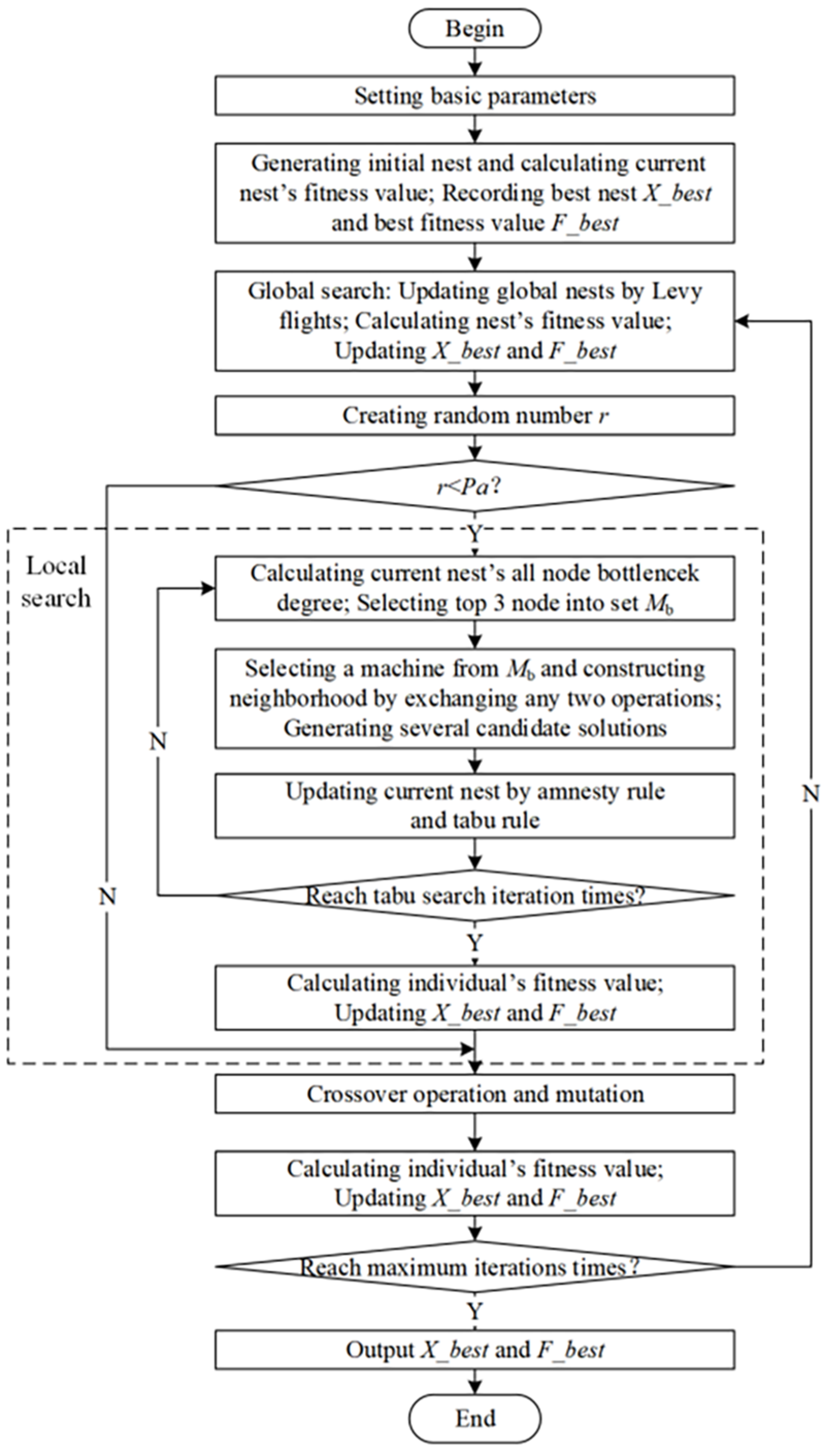
3. An Improved Cuckoo Search Algorithm under Bottleneck-Degree-Based Search Guidance, TSCS-BD

The cuckoo search algorithm is a meta-heuristic algorithm proposed by Yang and Deb [32]. It has the advantage of powerful searching ability and can effectively balance global and local searches. It is a widely used and successful algorithm in various engineering and management problems. It is applied to solve optimization problems by simulating the parasitic brooding behavior and flight characteristics of cuckoos. On one hand, the CS uses levy flight to find nests for breeding the next generation. On the other hand, the location of the nest is updated according to the probability of the eggs being discovered by the host bird. It offers two new solutions generated through global Levy flight random walk and local random walk. Levy flight obeys Levy probability distribution, with the search path consisting of frequent short jumps and occasional long jumps. This method can provide the CS algorithm with a larger search space. For large-scale optimization problems, the global search based on Levy flight is beneficial for exploring the algorithm over a wide range. However, the original local search strategy overlooks certain local optimization information, which leads to an algorithm prone to vibration in late running. Therefore, the local search strategy of the cuckoo search algorithm was replaced by adopting a tabu search. In addition, a construction strategy for the tabu search neighborhood structure under the search guidance of bottleneck degree was implemented to improve the searching ability of the algorithm. Neighborhoods were constructed by identifying machines with a high bottleneck degree and adjusting their schedules within the inter-cell manufacturing system. Bottleneck degree is used to guide the algorithm to optimize the search.

The flow chart of TSCS-BD is shown in Figure 1.

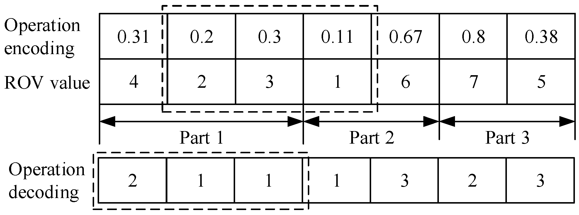
3.1. Coding and Decoding

A large-scale inter-cell scheduling problem is a discrete combinatorial optimization problem, which requires appropriate coding first. As the flight process of the cuckoo search algorithm is continuous rather than discrete, the numbers generated during the iteration process are not integers. Thus, it is necessary to employ an appropriate coding method to realize the conversion between discrete and continuous values.

Two-stage coding based on operation and machine is adopted. The first half of the coding represents the processing sequence of parts operation, based on a random-order value (ROV) encoding method [33]. The coding is non-integer and is converted into a decimal number arrangement to realize the sequence of operations in the decoding process. Each process is represented by the corresponding part’s serial number. Scanning the gene string from left to right, the serial number of the part appearing for the j-th time represents the j-th operation of the part. For example, there are three parts with three, two, and two operations, respectively, as shown in Figure 2. Then, seven natural numbers between 0–1 are randomly generated, such as 0.31, 0.2, 0.3, 0.11, 0.67, 0.8, 0.38. The numbers are arranged to generate corresponding ROVs, and the operations of the parts are arranged sequentially. The first 3 ROVs are circled with dashed square to represent O₂₁, O₁₁, and O₁₂.

The second half of the coding scheme represents selection of machines for parts. A direct coding method is adopted, as it does not perform Levy flights. The machine code is shown as Figure 3; O₁₁, O₁₂, and O₁₃ are processed by M₂, M₁, and M₃ respectively.

3.2. Global Search

CS is designed to obtain the best solution by simulating the foraging pattern of cuckoos, which models a random walk. The core strategy of CS is Levy flight, which is used for global search. Levy flight is a random walk mechanism that represents a type of Gaussian random process associated with a Levy stable distribution. The search path direction and step size change according to the Levy distribution, enabling the CS to explore the whole target space over a wide range. During the global random search, all nests except the optimal ones are updated. The Levy flight is executed using Equation (6) to update the discrete values and generate the position of the nest after the global random walk:

$$x_i^{t+1}=x_i^t+\alpha ⨂S$$

(6)

where $x_i^t$ represents the location of the i bird’s nest in the t generation; the scaling factor of step size is represented by α, in this paper, α = 1; ς represents the dot product of two vectors; S is the random walk step size subject to Levy distribution. The Mantegna algorithm [34] is used to perform Levy flight, and the specific step size S can be expressed by Equation (7):

$$S=\frac{\mu }{{\left|v\right|}^{1/\beta }}$$

(7)

where β is a parameter with a value range between [1, 2], in this paper, β = 1.5; $\mu \mathrm{and} v$ obey normal distribution, as shown in Equation (8):

$$\mu ~ N\left(0,{\sigma }_N^2\right), v~ N\left(0,{\sigma }_v^2\right)$$

(8)

Among them:

$$\begin{gathered} {\sigma }_N={\left\{\frac{\Gamma \left(1+\beta \right)sin\left(\pi \beta /2\right)}{\beta \Gamma \left[\left(1+\beta \right)/2\right]2^{\left(\beta -1\right)/2}}\right\}}^{1/\beta } \\ {\sigma }_v=1 \end{gathered}$$

3.3. Tabu Search under Bottleneck-Degree Guidance

In the local search within the CS, random numbers r ∈ (0, 1). When r < $P_a$, the nest is updated and a new nest is generated to replace the nest in a poor position, to carry out a local search within the CS. $P_a$ is the probability of a local search being successful (the probability of an egg being found in a nest). However, this relatively coarse local search neglects a considerable amount of local optimization information, resulting in slow convergence speed and low search accuracy when solving large-scale problems [35]. Therefore, in the local search, tabu search is proposed to replace the original local search strategy to improve the local searching ability of the algorithm.

3.3.1. Tabu Search

Tabu search [36] is an iterative search algorithm based on a local neighborhood search strategy, which realizes movement of feasible solutions through neighborhood construction. At the same time, once local optimal solutions have been found, they are stored in a table and selectively avoided in the next search, which improves the search efficiency of the algorithm. Tabu search generally includes the following basic elements: initial solution, neighborhood structure, tabu object, tabu table, tabu length, amnesty rule, and termination rule. Among them, neighborhood structure is the key step of the tabu search algorithm. In large-scale inter-cell scheduling problems, the solution space increases sharply, resulting in a decrease of searching efficiency in the random neighborhood structure. Therefore, bottleneck-degree guidance for a tabu search neighborhood structure is proposed.

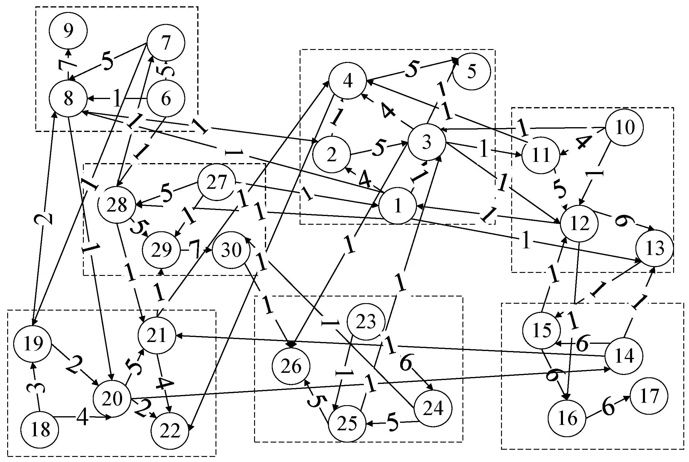
3.3.2. Complex Network Model and Bottleneck Degree

With increasing manufacturing tasks and resources, there may be a lot of constraints relating to machines and tasks in an inter-cell manufacturing system, which can be regarded as a complex system. To describe complex scheduling relationships in inter-cell manufacturing and seek abundant network features for scheduling optimization, a complex network model was established taking machines as nodes and the processing sequence among machines as bridges. Each obtained schedule corresponds to a specific complex network. A network G can be denoted G = (V, L) with node set V and edge set L, where node set V = {k|k = 1, 2, 3, …, m}. In this paper, G is a directed weighted network. The edge set can be expressed as E = {e_ij|i, j (1, 2, 3, ..., m)} where e_ij represents the edge from i to j. The expression of network elements should be clarified:

(1)

Nodes are the basic elements of the network model, which denote the machines.

(2)

Edges are the connections between nodes, which denote the flow of parts among machines.

(3)

Edge direction denotes the sequence of operations.

(4)

Weights denote the numbers of parts flowing between two machines.

As shown in Figure 4, there are seven cells, 30 machines, and 50 parts in the complex network model for a schedule. Each dashed box represents a separate manufacturing cell, the number on the node represents which machine it is, the directed edge represents the direction and flow of parts between machines, and the number on the directed edge represents the numbers of the parts flowing between two machines. For example, the number 4 on the directed line between machine 1 and machine 2 indicates that four parts flow to machine 2 for processing after machine 1 finishes processing.

The bottleneck degree is a composite index composed of complex network features. It can be used to measure the possibility of each node becoming a bottleneck under the combined influence of external manufacturing demand and internal production environment. It depends on attributes of the node itself, network propagation mechanism, and network topology, which are represented by three complex network features: node load, network efficiency, and betweenness centrality [37]. The symbols involved are shown in

Table 2. Parameters of complex network features.

Parameter	Parameter Meaning
$w_m$	Node load of node m
$l_{st}$	The shortest distance between nodes s and t
$e_{st}$	Network efficiency between nodes s and t
${\delta }_{st}$	Number of shortest paths from node s to node t
${\delta }_{stm}$	Number of shortest paths from node s to node t through node m
$b_m$	Betweenness centrality of node m
$s_m$	Bottleneck degree of node m

. The larger the bottleneck degree of the node, the more important the corresponding machine is in the manufacturing system. The bottleneck degree of node m is shown by Equation (9):

$$s_m=\frac{b_m{{\displaystyle \sum }}_{t=1}^M{e}_{mt}{w}_m}{{{\displaystyle \sum }}_{m’=1}^M{b}_{m’}{{\displaystyle \sum }}_{t=1}^M{e}_{m’t}{w}_{m’}}$$

(9)

As shown in Equation (10), node load $w_m$ represents the ratio of the total processing time of all parts on the node machine to the total processing time of all parts in the system. A larger node load on a node machine indicates that a lot of parts are processed on it. $a_{ijm}$ represents whether operation $O_{\mathrm{ij}}$ is processed on machine $m$, and $T_{ijm}$ represents the processing time of operation $O_{\mathrm{ij}}$ on machine $m$.

$$w_m=\frac{{{\displaystyle \sum }}_{i=1}^N{{\displaystyle \sum }}_{j=1}^J{a}_{ijm}{T}_{ijm}}{{{\displaystyle \sum }}_{m’=1}^M{{\displaystyle \sum }}_{i=1}^N{{\displaystyle \sum }}_{j=1}^J{a}_{ijm’}{T}_{ijm’}}$$

(10)

The shortest path between any two nodes s and t is defined as the shortest path $l_{\mathrm{st}}$, which reflects the closeness of the two nodes. Network efficiency $e_{\mathrm{st}}$ is defined as the reciprocal of $l_{\mathrm{st}}$, which can measure the degree of interaction between node machines. As shown in Equation (11), when $e_{\mathrm{st}}=$0 (no path between two nodes), it indicates the two node machines do not correlate in the manufacturing system, and operations can be simultaneously processed; while $e_{\mathrm{st}}=$1 indicates the two node machines have a strong correlation, and operations are processed with sequence constraints.

$$e_{st}=\left\{\begin{array}{c}\frac{1}{l_{\mathrm{st}}} \mathrm{There} \mathrm{is} \mathrm{at} \mathrm{least} \mathrm{one} \mathrm{path} \mathrm{between} \mathrm{nodes} s \mathrm{and} t\\ 0 \mathrm{There} \mathrm{is} \mathrm{no} \mathrm{path} \mathrm{between} \mathrm{nodes} s \mathrm{and} t \end{array}\right.$$

(11)

As shown in Equation (12), betweenness centrality $b_m$ measures how often a node appears on the shortest paths between all pairs of nodes in the network, which describes the centrality of nodes in the overall network. The more interlocutions of nodes, the higher the probability of processing tasks flowing through the node machine.

$$b_m={{\displaystyle \sum }}_{s\ne m\ne t}^M\frac{{\delta }_{stm}}{{\delta }_{st}}$$

(12)

According to theory of constraints (TOC) [38], bottleneck generally refers to the key limiting factor in the whole. In manufacturing, the rationality of the schedule for the bottleneck machine has a great impact on the whole scheduling scheme. The machine load is usually taken as a metric for identifying bottleneck [39]. However, the method of determining the bottleneck degree of a node by relying solely on the node load index is not comprehensive enough. It focuses too much on the single node load and ignores the influence of other node machines. Therefore, the importance of a node machine in the manufacturing system is measured comprehensively from three aspects: node attributes, network topology structure, and network propagation mechanism, by using complex network theory.

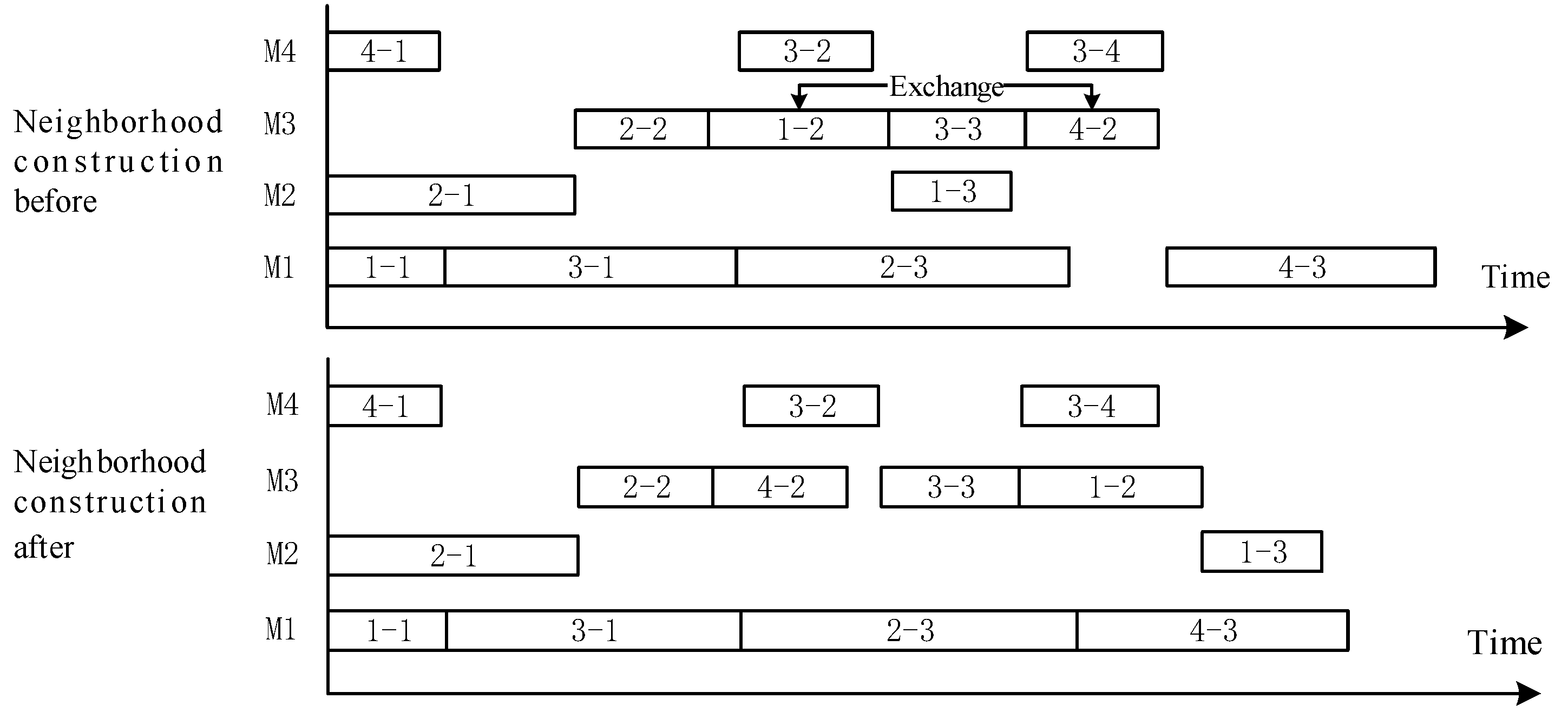
3.3.3. Bottleneck-Degree Guidance for Tabu Search Neighborhood Structure

In large-scale inter-cell scheduling, as the problem size increases, the solution space increases sharply, which leads to the decrease in the searching efficiency of the random neighborhood structure. The bottleneck machine plays a decisive role in the scheduling scheme. Therefore, targeted identification of bottleneck machines and construction of neighborhood structure can reduce the search scope of low-quality solution space and improve the overall search efficiency of the algorithm. The bottleneck degree can effectively identify the possibility that the node machine becomes a bottleneck. During the neighborhood construction stage, bottleneck machines are identified by calculating and sorting their bottleneck degree. Subsequently, candidate solutions are constructed by exchanging their positions within the sequential processing sequence.

The specific steps are as follows:

(1)

Selecting an individual to calculate the bottleneck degree with a $P_a$ probability;

(2)

Sorting each machine according to the bottleneck degree, with the first three machines with the highest bottleneck degree regarded as bottleneck machines $M_b$ in the current solution;

(3)

Randomly selecting one machine from $M_b$, and constructing the corresponding candidate solution by exchanging the position of any two operations processed on the machine with constraints;

(4)

Repeating step (3) until enough candidate solutions are generated.

In Figure 5, 1–1 represents the operation O₁₁, the first operation of part 1. Assuming machine M₃ is calculated to be a bottleneck machine, randomly selecting two operations processed on M₃ and exchanging their positions, other operations remain unchanged. A feasible candidate solution has been obtained. Repeat this step until enough candidate solutions are generated, especially giving preference to those candidate solutions which reduce the maximum completion time compared with the initial solution.

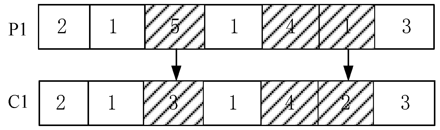
3.4. Crossover and Mutation

As exceptional parts have flexible routes, crossover and mutation are designed to ensure population diversity. For the machine-encoding segment, the multi-point preservative crossover (MPX) is applied. As shown in Figure 6, P₁ and P₂ represent two machine-encoding segments, and the shaded sections represent the coding bits of machines that processed exceptional operations. a set S composed of 0s and 1s is randomly generated, the length of the set equal to the number of exceptional parts, in which 0 indicates no action and 1 indicates crossover accepted. In encoding, exceptional parts and their machines are known, so the positions on the set correspond to the coding bits of the machine. Moreover, based on the position of 1 in the set S, determining the coding bits of the exceptional parts machines in the parents 1 and 2, and exchanging machines while other machines remain unchanged, the child encodings 1 and 2 are generated. The crossover is applied to exceptional parts, and alternative machines are known, so it will not change the constraints of operations of a given part, and the child encodings are all feasible solutions.

The mutation operation is also applied to the machine-encoding segment, firstly randomly selecting the machine code bits of several exceptional parts. As the parts can use alternative machines, an optional machine was selected to replace the original coding, ensuring that the child encodings generated after the operation are feasible solutions. The specific operation is shown in Figure 7.

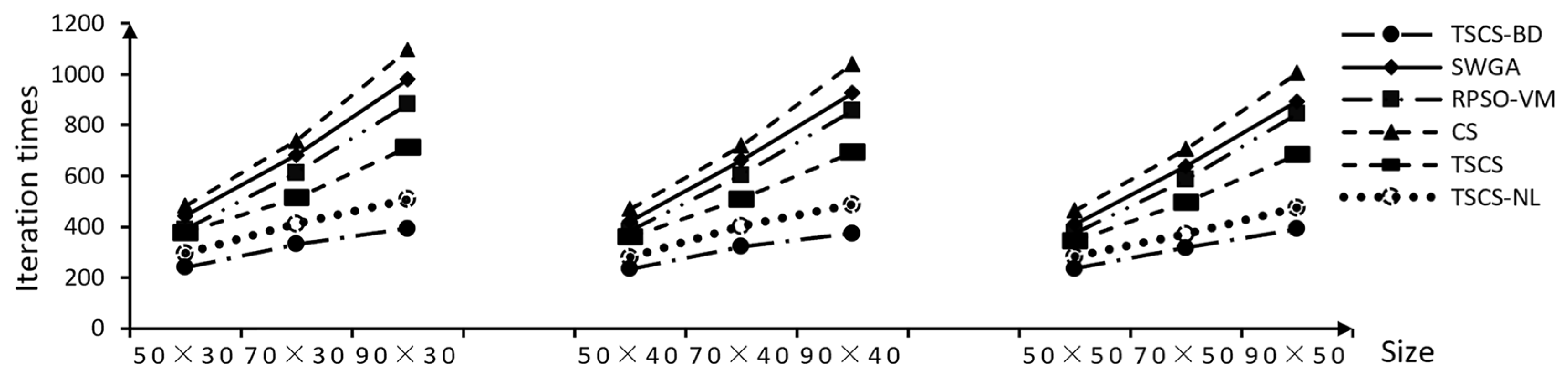
4. Experiments and Discussion

In order to verify the effects of the proposed TSCS-BD, nine large-scale inter-cell scheduling problems of different sizes were generated randomly. The results were compared with those yielded by a CS and two efficient large-scale optimization algorithms, a small-world genetic algorithm (SWGA) [15] and restart particle swarm optimization with velocity modulation (RPSO-VM) [40]. To verify the effects of the proposed bottleneck-degree guidance for the tabu search neighborhood structure, the results were compared with those yielded by an improved cuckoo search algorithm with general neighborhood structure (TSCS) and an improved cuckoo search algorithm with node-load guidance for neighborhood structure (TSCS-NL).

Parameters for the experiments were set as follows. Parts, machines, and manufacturing cells were randomly set from the ranges of 50–90, 30–50, and 7–12 respectively. Exceptional parts were randomly set from 15–25. Operations of parts were uniformly integer-distributed with range of [3, 6]. The processing times of operations were integers and obeyed normal distribution of N (30, 5). Each exceptional part had from three to seven alternative flexible routes for inter-cell movements. The experiments and parameters are shown in

Table 3. Summary of parameters for experiments.

Experiment	n × m	Cells	Exceptional Parts
L1	50 × 30	7	15
L2	70 × 30	7	15
L3	90 × 30	7	15
L4	50 × 40	9	20
L5	70 × 40	9	20
L6	90 × 40	9	20
L7	50 × 50	12	25
L8	70 × 50	12	25
L9	90 × 50	12	25

.

L1 is taken as an example; machines in manufacturing cells are shown in

Table 4. Machines in manufacturing cells.

Cell	Machines	Cell	Machines	Cell	Machines	Cell	Machines
U1	1, 2, 3, 4, 5	U2	6, 7, 8, 9	U3	10, 11, 12, 13	U4	14, 15, 16, 17
U5	18, 19, 20, 21, 22	U6	23, 24, 25, 26	U7	27, 28, 29, 30

. Parts, their candidate manufacturing cells, candidate processing machines, and processing time are shown in

Table 5. Parts processing time.

Parts	Manufacturing Cell, Processing Machines	Processing Time (min)
J1	$U_1\left(M_1,M_2,M_3,M_4,M_5\right)$	(29, 31, 26, 35, 37)
J2	$U_1\left(M_1,M_3,M_4,M_5\right)$	(27, 33, 34, 28)
⋮	⋮	⋮
J48	$U_7\left(M_{27},M_{28},M_{29},M_{30}\right)$	(27, 31, 22, 34)
J50	$U_7\left(M_{27},M_{28},M_{29},M_{30}\right)$	(28, 32, 28, 25)
Exceptional parts	Manufacturing Cell, Processing Machines	Processing Time (min)
J5	$U_1\left(M_1,M_2,M_3\right)+\left(\begin{array}{c}{U}_3\left(M_{11}\right)\\ U_4\left(M_{16}\right)\\ U_5\left(M_{20}\right)\end{array}\right)+U_1\left(M_4\right)$	$\left(25, 27, 27\right)+\left(\begin{array}{c}25\\ 27\\ 36\end{array}\right)+39$
⋮	⋮	⋮
J41	$U_6\left(M_{23},M_{24},M_{25}\right)+\left(\begin{array}{c}{U}_1\left(M_3\right)\\ U_2\left(M_7\right)\\ U_5\left(M_{20}\right)\\ U_7\left(M_{28}\right)\end{array}\right)+U_6\left(M_{26}\right)$	$\left(27, 24, 24\right)+\left(\begin{array}{c}31\\ 25\\ 26\\ 33\end{array}\right)+32$

. For example, operations of part J2 are processed on machines m₁, m₃, m₄, and m₅ of manufacturing cell U₁ and the processing times are 27, 33, 34, and 28 min respectively. Distances between machines in two different cells are shown in Figure 8. For example, the transportation time for parts between manufacturing cells U₁ and U₂ is 36 min.

Parameters for TSCS-BD, TSCS-NL, and TSCS were set as follows: nest size $N$ = 50, step factor $\alpha$ = 1, tabu rate $p_a$ = 0.1, length of tabu table $L$ = 10, times of iteration of tabu search $I_T$ = 6. In SWGA, population size $N$ = 50. In RPSO-VM, population size $N$ = 50, inertia weight $W$ = 0.5, learning factor $C_1$ = $C_2$ = 1.5. In CS, nest size $N$ = 50, step factor $\alpha$ = 1, nest detection rate $p_a$ = 0.1. For TSCS-BD, TSCS-NL, TSCS, SWGA, and CS, crossover rate $p_{\mathrm{c}}$ = 0.8, mutation rate $p_{\mathrm{m}}$ = 0.1. The number of iterations was set as 1500 generations. The termination condition was to reach the set maximum number of iterations or for solutions to remain unchanged within 120 generations.

To eliminate interference of random factors, the same experiments were conducted 10 times. Average makespan and average convergence iteration times are used for comparison. In order to show the effects of the proposed algorithm, completion time yielded by the TSCS-BD is used as a benchmark and compared with completion time yielded by other algorithms, as shown in Equation (13). P represents the percentage of average completion time better than the other algorithms. Comparison results are shown in

Table 6. Results and comparisons.

Example IS	TSCS-BD	SWGA		RPSO-VM		CS		TSCS		TSCS-NL
	Ctime	Ctime	P (%)	Ctime	P (%)	Ctime	P (%)	Ctime	P (%)	Ctime	P (%)
L1	402.2	441.7	8.94	448.3	10.32	475.3	15.38	418.1	3.80	429	6.25
L2	527.7	584.5	9.72	580.2	9.05	635.5	16.98	550.4	4.12	557.4	5.33
L3	654.1	728.3	10.19	721.4	9.33	795.3	17.74	685.7	4.61	673.7	2.91
L4	365.3	403.4	9.44	407.8	10.40	427.2	14.49	372.8	2.01	368.8	0.95
L5	469.5	521.3	9.94	528.5	11.16	564.4	16.81	482.3	2.65	500.3	6.16
L6	578.7	641.6	9.82	632.5	8.49	708.5	18.32	602.4	3.93	615.4	5.96
L7	348.3	379.1	8.20	389.1	10.46	411.7	15.38	356.2	2.22	359.2	3.03
L8	424.3	469.4	9.61	478.6	11.35	513.9	17.42	437.7	3.06	428.7	1.03
L9	507.7	562.7	9.79	572.3	11.29	618.7	17.94	526.3	3.53	529.3	4.08

, and iteration times for algorithms are shown in Figure 9.

$$\begin{gathered} P\left(X,IS\right)=\frac{C_{time}\left(X,IS\right)-C_{time}\left(TSCS-BD,IS\right)}{C_{time}\left(X,IS\right)}\times 100\% \\ X\in \left(SWGA,RPSO-VM,CS,TSCS, TSCS-NL\right) \end{gathered}$$

(13)

Table 6 clearly indicates that TSCS-BD yielded the best solutions among the algorithms for all of the nine examples. Among them, both TSCS-BD and TSCS are better than CS in terms of solution quality, indicating that the TS in TSCS-BD and TSCS could help CS to improve local searching ability compared with the original local search strategy. Moreover, bottleneck-degree guidance for the neighborhood structure in TSCS-BD could help the TS yield better quality solutions than the general neighborhood structure in TSCS. With increasing of part numbers in experiments with the same machine numbers, for example part numbers increased to 50, 70, and 90 in L1, L2, and L3, the solution quality of TSCS-BD is further improved compared with that of TSCS. This shows that the proposed bottleneck-degree guidance for the neighborhood structure in TSCS-BD is more suitable for large-scale problems than the general neighborhood structure in TSCS.

Figure 9 shows that the iteration times of TSCS-BD are the least among all the algorithms. It can be concluded that bottleneck-degree guidance for a TS in TSCS-BD can construct a neighborhood structure on machines with large bottleneck degree, which reduces the search scope of low-quality solution space and efficiently finds the descent direction of the algorithm within less iteration time. Therefore, TSCS-BD is effective for large-scale inter-cell scheduling problems.

In addition, comparisons between TSCS-BD and TSCS-NL in Table 6 show that bottleneck-degree guidance for neighborhood structure can help the algorithm yield better solutions than node-load guidance. In order to further analyze the relationship and difference between bottleneck degree and node load, L1 is taken as an example to analyze complex network features associated with bottleneck degree (Figure 4). Machines are sorted in descending order according to complex network features, as shown in

Table 7. Complex network features analysis for L1.

Rank	1	2	3	4	5	6	7	8	9	10
Bottleneck Degree	M12 1.00	M1 0.98	M3 0.67	M8 0.43	M28 0.28	M20 0.27	M15 0.23	M14 0.18	M25 0.13	M2 0.13
Node Load	M12 1.00	M4 0.94	M30 0.92	M8 0.90	M26 0.86	M13 0.86	M20 0.84	M14 0.84	M16 0.80	M1 0.80
Network Efficiency	M1 1.00	M27 0.85	M3 0.85	M12 0.81	M14 0.79	M8 0.78	M10 0.75	M6 0.73	M28 0.72	M11 0.69
Betweenness Centrality	M12 1.00	M1 0.89	M3 0.73	M8 0.49	M28 0.38	M20 0.35	M15 0.34	M25 0.23	M2 0.23	M14 0.22
Rank	11	12	13	14	15	16	17	18	19	20
Bottleneck Degree	M7 0.08	M21 0.06	M13 0.04	M19 0.03	M4 0.02	M29 0.02	M16 0.01	M30 0.01	M11 0.01	M24 0.01
Node Load	M6 0.76	M21 0.76	M3 0.75	M15 0.75	M18 0.73	M23 0.73	M27 0.66	M28 0.66	M22 0.65	M29 0.65
Network Efficiency	M20 0.69	M19 0.67	M18 0.67	M25 0.65	M2 0.64	M23 0.64	M15 0.63	M7 0.63	M24 0.60	M13 0.49
Betweenness Centrality	M7 0.16	M21 0.16	M29 0.13	M16 0.11	M4 0.10	M19 0.07	M13 0.06	M30 0.04	M24 0.01	M11 0.01
Rank	21	22	23	24	25	26	27	28	29	30
Bottleneck Degree	M26 0.00	M17 0.00	M27 0.00	M6 0.00	M5 0.00	M9 0.00	M10 0.00	M23 0.00	M18 0.00	M22 0.00
Node Load	M5 0.63	M9 0.61	M10 0.57	M11 0.52	M17 0.44	M25 0.43	M2 0.43	M24 0.34	M7 0.34	M19 0.00
Network Efficiency	M21 0.35	M4 0.16	M29 0.12	M16 0.08	M30 0.08	M22 0.00	M17 0.00	M26 0.00	M9 0.00	M5 0.00
Betweenness Centrality	M22 0.00	M26 0.00	M5 0.00	M6 0.00	M27 0.00	M10 0.00	M23 0.00	M18 0.00	M17 0.00	M9 0.00

.

The top five node machines in Table 7 sorted by bottleneck degree are M₁₂, M₁, M₃, M₈, and M₂₈, and the top five node machines sorted by node load are M₁₂, M₄, M₃₀, M₈, and M₂₆. Among them, both the bottleneck degree and the node load of M₁₂ and M₈ are large. This shows that bottleneck degree has a correlation with node load. Both of them could reflect the importance of the machines to a certain extent. However, the bottleneck degrees of M₄, M₃₀, and M₂₆ are not large compared with the other nodes. According to Equation (9), this is because the network efficiency and betweenness centrality of M₄, M₃₀, and M₂₆ are small. Taking the complex network model for L1 in Figure 4 as an example, M₃₀ has no outgoing edges, indicating that the machine mainly processes the last process of the parts. This type of machine has less impact on other machines and is less important than the others. Therefore, the node load itself cannot adequately reflect the roles of machines in the manufacturing system. In addition, the bottleneck degrees of M₁, M₃, and M₂₈ are large but they have small node loads, which is because the network efficiency and betweenness centrality of M₁, M₃, and M₂₈ are large. M₃ in Figure 4 connects with nine directed edges and 14 nodes (including second-order neighbor nodes), which is higher than the average of the machines connected with four directed edges and 8 nodes. Although there are few operations processed on M₃, it associates with many machines and has great impact on the processes of other machines. This type of machine remains important in the manufacturing system. Therefore, bottleneck degree considers not only node load but also interaction between machines in processing tasks, which is a better indicator than node load to measure the importance of machines in manufacturing systems.

5. Conclusions

In order to solve large-scale inter-cell scheduling optimization problems, an inter-cell scheduling optimization model aiming at minimizing the maximum completion time has been established. An improved cuckoo search algorithm under bottleneck-degree-based search guidance is proposed, using complex network features to guide algorithm improvement. Tabu search was introduced into the cuckoo search algorithm to replace the original local search strategy, and bottleneck degree is used to guide the design of the neighborhood structure in the tabu search. This improves the optimization efficiency of the tabu search and then improves the overall optimization efficiency and solving quality of the algorithm. Through the comparisons of different scale examples, the feasibility and superiority of the improved cuckoo search algorithm under bottleneck-degree-based search guidance for solving large-scale inter-cell scheduling problems are illustrated.

There are still some limitations that need further study. Initial solutions are not improved using the algorithm. In the future, initial solutions can be screened to improve the effect of the algorithm. Preprocessing of scheduling problems can be combined with algorithm improvement to further improve the optimization effect. In addition, correlation between other complex network features and scheduling optimization can be further explored to yield better optimization results.

References

1. Manuel, S.; Sophie, N.P. Solving large scale industrial production scheduling problems with complex constraints: An overview of the state-of-the-art. Procedia Comput. Sci. 2023, 217, 1028–1037. [Google Scholar]
2. Mahdavi, S.; Shiri, M.E.; Rahnamayan, S. Metaheuristics in large-scale global continues optimization: A survey. Inf. Sci. 2015, 295, 407–428. [Google Scholar] [CrossRef]
3. Feng, Y.; Li, G.; Suresh, P.S. A three-layer chromosome genetic algorithm for multi-cell scheduling with flexible routes and machine sharing. Int. J. Prod. Econ. 2018, 196, 269–283. [Google Scholar] [CrossRef]
4. Zhang, R.; Wu, C. A divide-and-conquer strategy with particle swarm optimization for the job shop schedule problem. Eng. Optim. 2010, 42, 641–670. [Google Scholar] [CrossRef]
5. Wu, D.; Ierapetritou, M.G. Decomposition approaches for the efficient solution of short-term schedule problems. Comput. Chem. Eng. 2003, 27, 1261–1276. [Google Scholar] [CrossRef]
6. El-Kholany, M.M.S.; Gebser, M.; Schekotihin, K. Problem Decomposition and Multi-shot ASP Solving for Job-shop Scheduling. Theory Pract. Log. Program. 2022, 22, 623–639. [Google Scholar] [CrossRef]
7. Chu, C.; Portmann, M.C.; Proth, J.M. A splitting-up approach to simplify job-shop schedule problems. Int. J. Prod. Res. 1992, 30, 859–870. [Google Scholar] [CrossRef]
8. Zuo, Y.; Gu, H.; Xi, Y. Study on constraint scheduling algorithm for job shop problems with multiple constraint machines. Int. J. Prod. Res. 2008, 46, 4785–4801. [Google Scholar] [CrossRef]
9. Sannomiya, N.; Lima, H. Genetic algorithm approach to an optimal scheduling problem for a large-scale complex manufacturing system. In Proceedings of the IEEE International Conference on Systems, Man, and Cybernetics, Tokyo, Japan, 12–15 October 1999; Volume 3, pp. 622–627. [Google Scholar]
10. Roslöf, J.; Harjunkoski, I. A short-term scheduling problem in the paper-converting industry. Comput. Chem. Eng. 1999, 23, 871–874. [Google Scholar] [CrossRef]
11. Roslöf, J.; Harjunkoski, I. Solving a large-scale industrial scheduling problem using MILP combined with a heuristic procedure. Eur. J. Oper. Res. 2002, 138, 29–42. [Google Scholar] [CrossRef]
12. Yang, F.; Gao, K.; Simon, I.W. Decomposition methods for manufacturing system scheduling: A survey. IEEE/CAA J. Autom. Sin. 2018, 5, 389–400. [Google Scholar] [CrossRef]
13. Yuan, Y.; Xu, H. An integrated search heuristic for large-scale flexible job shop scheduling problems. Comput. Oper. Res. 2013, 40, 2864–2877. [Google Scholar] [CrossRef]
14. Li, Y.; Chen, X.; An, Y. Integrating machine layout, transporter allocation and worker assignment into job-shop scheduling solved by an improved non-dominated sorting genetic algorithm. Comput. Ind. Eng. 2023, 179, 109169. [Google Scholar] [CrossRef]
15. Cheng, R.; Jin, Y. A Competitive Swarm Optimizer for Large Scale Optimization. IEEE Trans. Cybern. 2014, 45, 191–204. [Google Scholar] [CrossRef] [PubMed]
16. Ali, K.B.; Telmoudi, A.J.; Gattoufi, S. Improved Genetic Algorithm Approach Based on New Virtual Crossover Operators for Dynamic Job Shop Scheduling. IEEE Access 2020, 8, 213318–213329. [Google Scholar] [CrossRef]
17. Qiao, Y.; Wu, N.; He, Y. Adaptive genetic algorithm for two-stage hybrid flow-shop scheduling with sequence-independent setup time and no-interruption requirement. Expert Syst. Appl. 2022, 208, 118068. [Google Scholar] [CrossRef]
18. Gao, K.; Cao, Z.; Zhang, L. A review on swarm intelligence and evolutionary algorithms for solving flexible job shop scheduling problems. IEEE/CAA J. Autom. Sin. 2019, 6, 904–916. [Google Scholar] [CrossRef]
19. Xie, J.; Li, X.; Gao, L. A hybrid algorithm with a new neighborhood structure for job shop scheduling problems. Comput. Ind. Eng. 2022, 169, 108205. [Google Scholar] [CrossRef]
20. Sun, K.; Zheng, D.; Song, H. Hybrid genetic algorithm with variable neighborhood search for flexible job shop scheduling problem in a machining system. Expert Syst. Appl. 2023, 215, 119359. [Google Scholar] [CrossRef]
21. Majumder, A.; Laha, D.; Suganthan, P.N. A hybrid cuckoo search algorithm in parallel batch processing machines with unequal job ready times. Comput. Ind. Eng. 2018, 124, 65–76. [Google Scholar] [CrossRef]
22. Alon, U. Biological networks: The tinkerer as an engineer. Science 2003, 301, 1866–1867. [Google Scholar] [CrossRef]
23. Bray, D. Molecular networks: The top-down view. Science 2003, 301, 1864–1865. [Google Scholar] [CrossRef] [PubMed]
24. Newman, M.E.J. The structure and function of complex networks. SIAM Rev. 2003, 45, 167–256. [Google Scholar] [CrossRef]
25. Barabási, A.L. Emergence of scaling in random networks. Science 1999, 286, 509–512. [Google Scholar] [CrossRef] [PubMed]
26. Eric, S.; Michael, P.H.S. Complex networks and simple models in biology. J. R. Soc. Interface 2005, 2, 16849202. [Google Scholar]
27. Zhao, Y. Public Opinion Evolution Based on Complex Networks. Cybern. Inf. Technol. 2015, 15, 55–68. [Google Scholar] [CrossRef]
28. Rajapakse, I.; Groudline, M.; Mehran, M. Dynamics and control of state-dependent networks for probing genomic organization. Proc. Natl. Acad. Sci. USA 2011, 108, 17257–17262. [Google Scholar] [CrossRef]
29. Becker, T.; Wagner, D. Identification of key machines in complex production networks. Procedia CIRP 2016, 41, 69–74. [Google Scholar] [CrossRef]
30. Pang, H.; Jiang, X. Solution of Flexible Job Shop Scheduling Problem Based on Ant Colony Algorithm and Complex Network. In Proceedings of the 10th International Symposium on Computational Intelligence and Design, Hangzhou, China, 9–10 December 2017; pp. 463–466. [Google Scholar]
31. Zou, M.; Liu, Q.; Yin, Y. Improved small world genetic algorithm for intercell scheduling in network environment. Comput. Integr. Manuf. Syst. 2019, 25, 1991–1999. [Google Scholar]
32. Yang, X.S.; Deb, S. Cuckoo search via Lévy flight. In Proceedings of the World Congress on Nature & Biologically Inspired Computing, Coimbatore, India, 9–11 December 2009; pp. 210–214. [Google Scholar]
33. Bean, J.C. Genetic Algorithms and Random Keys for Sequencing and Optimization. ORSA J. Comput. 1994, 6, 154–160. [Google Scholar] [CrossRef]
34. Mantegna, R.N. Fast accurate algorithm for numerical simulation of Lévy stable stochastic processes. Phys. Rev. E 1994, 49, 4677. [Google Scholar] [CrossRef] [PubMed]
35. Sadiq, M.S.; Feras, C.O.; Abdalrahman, M.A. Engineering a Memetic Algorithm from Discrete Cuckoo Search and Tabu Search for Cell Assignment of Hybrid Nanoscale CMOL Circuits. J. Circuits Syst. Comput. 2016, 25, 1650023. [Google Scholar]
36. Glover, F. Tabu Search: A Tutorial. Inf. J. Appl. Anal. 1990, 20, 74–94. [Google Scholar] [CrossRef]
37. Li, X.; Yuan, Y.; Sun, W. Bottleneck identification in job-shop based on network structure characteristic. Comput. Integr. Manuf. Syst. 2016, 22, 1088–1096. [Google Scholar]
38. Golmohammadi, D. A study of scheduling under the theory of constraints. Int. J. Prod. Econ. 2015, 165, 38–50. [Google Scholar] [CrossRef]
39. Zou, Y.; Gu, H.; Xi, Y. Modified bottleneck-based heuristic for large-scale job-shop scheduling problems with a single bottleneck. J. Syst. Eng. Electron. 2007, 18, 556–565. [Google Scholar]
40. Nieto, J.G.; Alba, E. Restart particle swarm optimization with velocity modulation: A scalability test. Soft Comput. 2011, 15, 2221–2232. [Google Scholar] [CrossRef]
Figure 1. Flow chart of TSCS-BD.
Applsci 14 01011 g001
Figure 2. Encoding and decoding rule based on ROV.
Applsci 14 01011 g002
Figure 3. Two-stage coding based on operation and machine.
Applsci 14 01011 g003
Figure 4. Complex network model of inter-cell manufacturing system.
Applsci 14 01011 g004
Figure 5. Neighborhood structure construction.
Applsci 14 01011 g005
Figure 6. Crossover operation of machine encoding segments.
Applsci 14 01011 g006
Figure 7. Mutation operation of machine-encoding segments.
Applsci 14 01011 g007
Figure 8. Distance matrix (numbers are time needed for transportation between two cells in the same vehicles at the same speed).
Applsci 14 01011 g008
Figure 9. Comparisons of iteration times.
Applsci 14 01011 g009