Tibia-YOLO: An AssistedDetection System Combined with Industrial CT Equipment for Leg Diseases in Broilers

Abstract

With the continuous improvement of broiler production performance, the frequent occurrence of leg problems has caused serious economic losses in many factories. In order to more efficiently detect and prevent broiler leg diseases, we propose an auxiliary detection system for broiler leg diseases based on deep learning. The system is divided into two parts. First, a digital radiography (DR) image of a broiler is taken through industrial computed tomography (CT), and then the improved deep-learning network Tibia-YOLO is used to detect the tibia; the detected results are then extracted and measured. Our improved Tibia-YOLO network uses the Content-Aware ReAssembly of Features (CARAFE) upsampling operator to avoid checkerboard artifacts and increase the generalization capabilities. Efficient multi-scale attention (EMA) and parallel network attention (ParNet) were added to the Tibia dataset at multiple scales (COCO2016), and there were improvements when testing on the three VOC2012 datasets. The mean average precision of tibia detection reached 90.8%, and the root mean square error (RMSE) for the tibia length was 3.37 mm.

1. Introduction

In the production process for broiler chickens, in order to reduce production costs enterprises have continuously improved the breeding technology for broilers, and their production performance has also improved. However, the rapid growth of the production of broilers has caused some problems, such as a significant increase in the incidence of leg diseases. According to statistics, approximately 14–30% of broiler chickens worldwide have leg diseases [1,2]. In many cases, due to the lack of timely attention, broiler leg problems have caused large-scale losses for companies. A key to detecting leg diseases in broilers is the measurement of the length of the tibia. The traditional measurement method requires the dissection of a broiler leg and the measurement of the length of the tibia with a vernier caliper or tape measure. This is very inefficient and detrimental to the leg health of the broiler. In summary, in the current broiler chicken breeding industry, an efficient and accurate system for measuring a broiler’s tibia is needed.

In order to minimize the damage to broiler chickens after they pass inspections and to avoid the damage caused by traditional measurement methods, we introduced a fast digital X-ray photography system for photographing broiler chickens and accurately and efficiently measuring their tibia. Digital radiography (DR) is a digitized imaging technique in the realm of medicine [3], and it represents a digital evolution of traditional radiology. Presently, the applications of DR extend beyond human medical fields to include animal healthcare [4] as well as industrial inspection [5], among other domains. When applied to the task of leg disorder detection in broiler chickens, it facilitates the rapid imaging of these birds. The generated DR images exhibit a remarkable ability to distinguish bone structures from other tissues, thus aiding in subsequent length measurement procedures. To minimize the operational costs for enterprises, all DR images employed in this study were sourced exclusively from industrial computed tomography (CT) equipment.

In order to solve the problem of measuring the length of the legs of broiler chickens, we designed a system for non-destructive measurement. The system consisted of two parts. The first part used industrial CT equipment to image the broiler chickens. The imaging process was very short and did not cause damage to the broiler chickens. The second part was the automatic determination of the leg tibia data contained in the broiler DR images based on deep learning. Using our improved Tibia-YOLO network, the tibia of a broiler’s leg could be detected efficiently and accurately. After the network extracted the detection bounding box of the tibia, it extracted the pixel length of the long side of that box. Support vector regression (SVR) was used to predict broiler chickens’ tibia lengths by using the pixel length. In the next part, we will discuss the difficulties encountered and solutions found during the process of improving the Tibia-YOLO network.

As the field of deep learning has advanced, convolutional neural networks (CNNs) have come into focus, with a growing number of researchers leveraging CNNs on publicly available datasets for object detection tasks and yielding commendable detection results [6]. Concurrently, the utilization of digital radiography (DR) images has significantly enhanced the efficiency of medical practitioners. For instance, in the realms of pulmonary disease screening [7] and fracture detection [8], deep-learning techniques have assisted healthcare professionals in promptly assessing potential maladies. Most models adopted in deep learning have a deeper depth, but they produce problems such as excessive sequential processing and more latency [9]. We chose the You Only Look Once (YOLO) series as a baseline because it is a single-stage target detection method that can process a network more efficiently.

In this study, to address the issue of increased sequential computations and higher latency in traditional object detection networks, we managed to significantly enhance the detection accuracy without introducing excessive sequential computations. In the YOLOv8 network, we used the Content-Aware Reassembly of Features (CARAFE) operator for feature fusion during feature upsampling [10]. We introduced the parallel network (ParNet) attention mechanism into the Backbone section [11], and we incorporated the efficient multi-scale attention (EMA) mechanism into multiple channels within the Neck [12]. At the same time, we used the Wise IoU (WIoU) [13] loss function. The end result was a significant increase in average precision (mAP) and a smaller root mean square error (RMSE).

Our contributions can be summarized as follows:

• We established a dataset of broiler tibias, and it included the bounding boxes of the tibias and the real lengths corresponding to them.
• On the basis of lightweight detection using YOLOv8-s, we introduced the ParNetAttention (ParNet) attention mechanism into the Backbone. This reduced the depth of the network and allowed it to better deal with long-distance dependencies, thus improving its overall performance.
• Efficient multi-scale attention (EMA) was introduced before each layer of the target detection head on the Neck. This helped to better highlight and extract the key features of these large targets, thus improving the efficiency of feature extraction and, ultimately, the detection accuracy.
• We used the Content-Aware Reassembly of Features (CARAFE) upsampling operator, which reduced the checkerboard artifact phenomenon, had a stronger data generalization ability, and allowed more semantic information to be obtained.
• The experiments showed that our method could effectively detect tibias, and when combined with a linear regression prediction model it could measure the length of a broiler tibia.

2. Related Work

Some researchers have used deep learning to determine length measurement. Dang, L. Minh et al. [14] used the deep-learning model DeepLabV3+ to detect cracks in public facilities made of concrete and asphalt, such as sewers and tunnels, and they measured the lengths of the cracks. Finally, an intersection-over-union (IoU) [15] score of 0.97 and an F1 score of 98% were obtained. Jung and Sang-Kyu [16] trained ResNet-V2-101 on 16,000 images of Caenorhabditis elegans and, finally, used AniLength to measure its length, with an average accuracy of 99.7%. Xiangyun Long et al. [17] proposed measuring the fatigue crack growth rate based on deep learning. The measurement equipment consisted mainly of a handheld mobile phone. After a comparison, the accuracy of predicting the crack length within 5% and 3% of the true length was 98.79% and 91.82%, respectively. Abdelaziz Triki et al. [18] used Mask R-CNN to segment plant leaves and measure their length and width. The measurement results were compared with those of manual measurements. The average error of the blade length was 4.6%, and the average error of the blade width was 5.7%. Marrable, Daniel et al. [19] proposed a semi-automatic measurement method based on deep learning for a three-dimensional decoy remote underwater video system. The results proved that the measured Pearson correlation coefficient (R) was 0.99. These measurement tasks were all based on common computer vision tasks. However, for some measurement targets that are invisible to the naked eye, this approach needs to be rethought.

We paid attention to non-invasive imaging technology to help us more accurately observe images of tibias from broilers’ legs and to aid in subsequent detection tasks based on deep learning. In the following, some applications of deep learning with DR images reported by other researchers are described. Kim, Min Jong et al. [20] used a deep-learning model, U-Net, with convolutional networks for biomedical image segmentation in combination with DR images to measure differences in human leg length. The Pearson correlation coefficient of the final result ranged from 0.880 to 0.996. This can save much labor for medical workers, and the calculation results were close to those of manual measurements. Xiaohua Wang et al. [21] screened 1881 chest DR images for pneumoconiosis and used the CNN of Inception-V3 for recognition testing. The final result for the area under the receiver operating characteristic curve (AUC) was 0.878, which was higher than the AUC of the screening results from two radiologists. Feng, Qi et al. [22] measured the length, depth, and other indicators of the ears of sella turcica in DR images of their heads; they segmented the parts of sella turcica with a deep-learning model (U-net) and then used an open-source computer vision library (OpenCV) to obtain the corresponding coordinates and assess the length, depth, and other indicators. The final measurements were very close to the manual measurements. Patil, Vathsala, et al. [23] used the medical X-ray images of 1000 teeth and found that the mesial root length of the right third molar could be used to predict age very well, and the accuracy with a support vector machine (SVM) reached 86.4%. We found that researchers have rarely paid attention to issues of speed and weight when operating deep-learning networks.

The YOLO series is a single-stage target detection method with a more efficient processing network. Some researchers have used detectors involving the YOLO series for agricultural, medical, and industrial applications. Mino Sportelli et al. [24] used YOLO detectors to detect weeds on farmland, thus reducing human workload. Kaile Jiang et al. [25] used the improved YOLOv5 to identify and count postoperative surgical instruments to prevent medical accidents. Huilong Jin et al. [26] used YOLOv5 to detect scratches and torn gloves during the industrial production of medical gloves. Several researchers reported applications of the YOLOv8 network in many industries. Haiwei Chen et al. [27] proposed the C2f, and the average accuracy was greatly improved. Bingjie Xiao et al. [28] used YOLOv8 to classify fruits in digital images. Compared with the CenterNet model, they proved that YOLOv8 was significantly better in the tasks of feature extraction and fruit classification in fruit images. Haoyu Jiang et al. [29] improved on the basis of YOLOv8-n; by introducing the C2f-Ghost structure and depth-separable convolution, they reduced the computational complexity of the model and compressed the model size. They proposed the YOLOv8-Pears model, which was able to analyze and quantify the germination activity of different genotypes of peas and select the most drought-resistant pea varieties. Tingting Yang et al. [30] proposed YOLOv8 and the improved DeepLabv3+, and they used a fused network to achieve higher accuracy on a public leaf dataset. Compared with traditional segmentation methods, this fusion network significantly improved the segmentation performance. Wenjie Yang et al. [31] used deformed convolution and coordinated attention to improve YOLOv8 and enhance the architecture of YOLOv8. The model was tested on a dataset collected from a cattle farm and ultimately achieved good results in terms of both speed and accuracy.

To summarize, we chose to improve the YOLOv8 network. The main goal was to improve the accuracy of the bounding box during tibia detection in the DR images of broilers. Finally, the length of the bounding box was used to fit and predict the length of the tibia, thus providing farm workers with more valuable leg data, preventing leg diseases in broiler chickens, and avoiding large-scale losses in the breeding industry. In order to make the model’s final prediction of the tibia length more accurate, we needed to improve the accuracy of the deep-learning network.

3. Materials and Methods

We used the Tibia-YOLO model improved based on YOLOv8-s to detect the tibia of broiler chicken legs. We extracted the height pixel value from the detection results and used the SVR regression model to predict the tibia of broiler chicken legs. In Section 3.1, we will introduce the creation process of the tibia dataset and two public datasets. In Section 3.2, we will introduce the structure of the Tibia-YOLO target detection network. In Section 3.3, we will introduce the SVR regression model. In Section 3.4, we will introduce the experimental setup and the setting of evaluation metrics.

3.1. Dataset

3.1.1. Tibia Dataset of DR Images

In this study, we scanned live broiler chickens with industrial CT equipment. During the data processing, the broiler chickens were placed in a dark environment and held in an inverted posture to capture DR images. Figure 1 depicts the collection of DR images. By manually screening and removing some DE images with large artifacts, a total of 228 DR images of broiler chickens were collected, and each image contained two complete broiler chicken leg areas. Each image was manually labeled by our team.

Due to the limited data from broiler DR images, deep learning could suffer from overfitting during the training process. Therefore, we performed data augmentation on the 228 original DR images of the 228 broiler chicken individuals to reduce the risk of overfitting in the network. We randomly used five methods—brightness adjustment, reflected noise, angle rotation, horizontal flipping, and translation—to process the original images and labels at the same time, and we finally obtained 2280 images and labeled data. The original DR images and enhanced images in the dataset are shown in Figure 1. In the process of dividing the dataset, we regarded the original DR images and the enhanced data as the source data of one broiler, and we did not distribute the enhanced images of the same broiler chicken among the training set, verification set, and test set. It was ensured that the broiler DR images in the validation set or test set were not used for pre-training. We randomly generated training sets, test sets, and validation sets based on individual broiler chickens, and we allocated 70% for training, 15% for testing, and 15% for validation.

Following the acquisition of DR images, in collaboration with professional slaughter personnel on-site, we conducted anatomical dissections of broiler legs and performed precise measurements using electronic calipers. Subsequently, we established a Tibia branch dataset tailored for the tibial regression model. The dissections involved 55 broilers, resulting in 110 leg samples, encompassing both DR images and tibial lengths. Out of these, 88 tibial length data points were allocated for the training set, while the remaining 22 were designated for testing purposes. Within this dataset, each DR image, as detected by the Tibia-YOLO model, yielded two leg regions, from which the pixel height of the detection box was extracted. Each pixel height corresponded to a true tibial length measured through anatomical dissection, expressed in millimeters. This branch dataset is amenable to supervised learning models. The chickens were slaughtered in a manner that complied with the requirements and was approved by the Experimental Animal Welfare and Animal Experimentation Ethical Review Committee of China Agricultural University.

3.1.2. PASCAL VOC2012 Dataset

To evaluate the performance of our proposed Tibia-YOLO model, we additionally used the object detection sub-dataset from the Visual Object Classes Challenge 2012 (VOC2012) dataset. These data included people, birds, and cats, as well as twenty object categories, such as dogs. The dataset contained 17,125 images. The label corresponding to each image included a bounding box and an object class label, and situations in which the same image appeared in multiple categories were also included.

3.1.3. COCO2016 Dataset

We additionally used the Microsoft Common Objects in Context 2016 (COCO2016) dataset to test the Tibia-YOLO model. The COCO2016 dataset contained more than 200,000 images and a total of 80 categories, including people, eight types of vehicles, and ten types of animals; more than 500,000 object entities were annotated.

3.2. Tibia-YOLO Network Structure

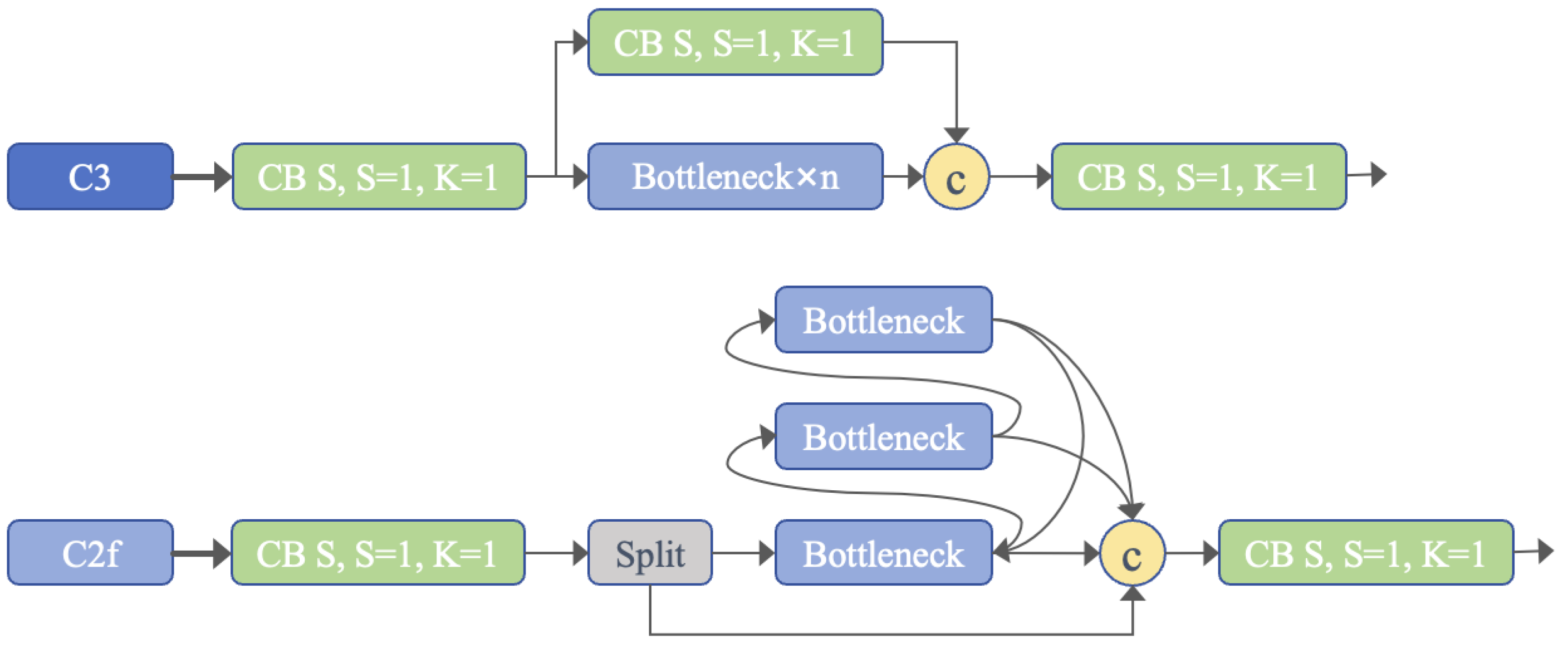
We used YOLOv8-s from the YOLO series as the baseline for improving the network. YOLOv8 uses a Backbone, making it similar to the YOLOv5 series. Unlike YOLOv5, the kernel of the first convolutional layer is changed from 6 × 6 to 3 × 3, and the CSPLayer structure is replaced with a cross-stage partial bottleneck with two convolutions (C2f) with richer gradient information. Traditional residual connections are usually adopted for the CSP, while DenseNet is used for C2f [32]; this introduces more skip layer connections, cancels the convolution operations within branches, and adds additional split operations. This design makes feature information richer while reducing the computational burden to ensure a balance between the two. The C2f module combines multiple advanced features and contextual information to effectively improve detection accuracy. A diagram of the structure of the C2f module is shown in Figure 2. In the output layer of YOLOv8, the sigmoid function was used as the activation function for the object score to represent the probability that the bounding box contained the detection object. The network used the softmax function to represent probability, which reflected the probability of each of the possible classes of the object. The Spatial Pyramid Pooling—Fast (SPPF) structure of the Backbone was used to handle objects of different scales. The SPPF structure used pooling kernels of different sizes to extract more features, used three consecutive poolings to reduce the amount of calculation, and combined the output of each layer to ensure multi-scale fusion while further expanding the receptive field and improving the speed at which the network operated. Different detectors at different levels of YOLOv8 were used to ensure that each detector was independently responsible for predicting the bounding box at one scale. This allowed YOLOv8 to increase its detection capabilities at different scales [33].

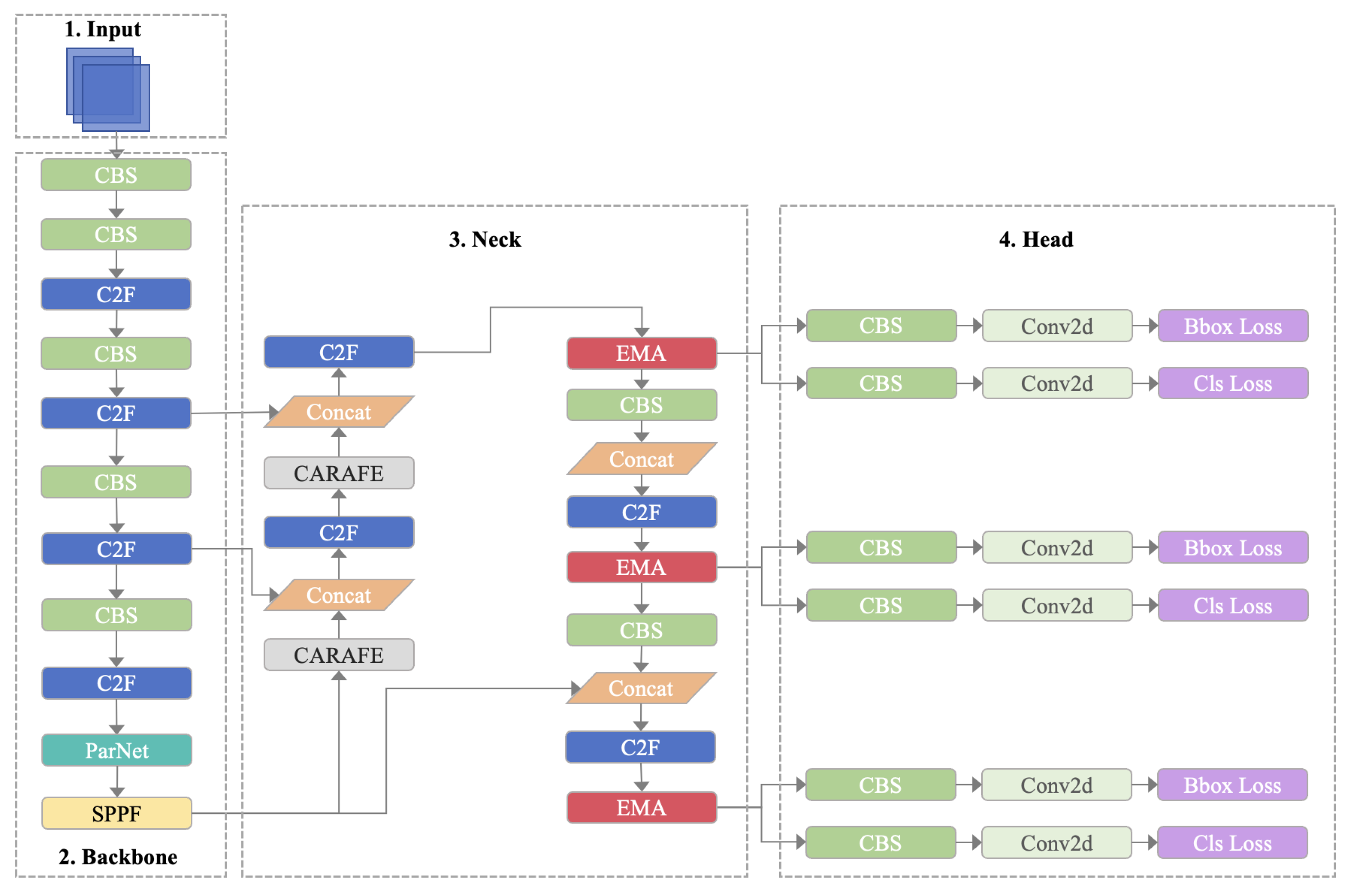
We used a target detection network based on YOLOv8, and the network structure included the Backbone, Neck, and Head. A multi-scale detection mechanism was introduced into YOLOv8. When detecting data in medical imaging formats, such as images of broiler tibias, the network could identify different sizes and structures and enhance the resolution of bone tissue and muscle tissue. At the same time, the YOLOv8 series is focused on real-time performance, which would help in its deployment in portable agricultural equipment. Compared with the results of the original YOLOv8, in order to improve the accuracy we used the CARAFE upsampling operator, which reduced checkerboard artifacts, ensured the availability of broiler DR images, and increased the generalization performance of the network. A parallel structure (ParNet) was added to the Backbone. This structure did not require more deep networks, could better handle long-distance dependencies, and could improve the overall performance of the network. In DR images of broiler legs, the tibia accounted for a large proportion; thus, this task was one of large-target detection. We also added the EMA attention mechanism at three different scales in the Neck, providing a stronger generalization ability and contributing to better detection. The key features of the large targets were highlighted and extracted. Our network architecture is shown in Figure 3.

3.2.1. Content-Aware Reassembly of Features

In deep neural networks, feature upsampling is a key issue, especially during feature fusion. Common upsampling methods include nearest-neighbor sampling and bilinear sampling. These sampling methods cannot capture more semantic information in processing-intensive tasks. Jiaqi Wang et al. proposed Content-Aware Reassembly of Features (CARAFE), which allows each pixel to generate multiple sets of global region weights and rearrange them to obtain upsampled features [10]. The core of CARAFE is an adaptive kernel generation mechanism. The upsampling kernel of the traditional upsampling method is fixed and cannot change as the input features change, but CARAFE can adjust the best upsampling effect based on the content. In the task of detecting broiler tibias, because some broilers are relatively active while DR images are taken, the generated images produce small numbers of artifacts, which cause the boundaries of bone tissue and muscle tissue in the images to become blurred, thus affecting the length measurements. Traditional upsampling uses transposed convolution, resulting in some checkerboard artifacts in the upsampling results, which would aggravate the degree of artifacts in the DR images of broiler legs. We chose the CARAFE upsampling operator to adaptively adjust the upsampling kernel and to effectively reduce these artifacts. At the same time, CARAFE can also regenerate new features during the upsampling process, effectively improving the accuracy and generalization ability of the target detection network, thus helping it to be deployed in auxiliary detection systems for more types of poultry animals.

First, during the process of reorganizing the kernel, CARAFE obtained a feature map from the previous Tibia-YOLO network. The resolution of this map was very low and contained many edges, color blocks, textures, and other information. There was a lightweight convolutional neural network in CARAFE. This network generated a unique upsampling kernel for different areas in the feature map, and it predicted a recombination kernel, $W_{l^{\prime }}$ (Formula (1)), based on the target content of each position, $l^{\prime }$. The content of these cores was dynamic and could change based on changes in the surrounding features.

$$W_{l^{\prime }}=\psi \left(N\left(x_l,k_{encoder}\right)\right)$$

(1)

The second step used the predicted features to reorganize (Formula (2)). This process involved spatial rearrangement and expansion of the feature map. Since the reorganization was determined for each region based on the dynamic kernel, each part of the feature map as a whole was related to the others, and the generated feature map also contained more information. Because the content generation of the kernel was content-based, CARAFE emphasized important semantic features during the upsampling process, and the detailed information and semantic information were also emphasized at larger scales. Overall, CARAFE is a highly adaptable upsampling method with detailed processing capabilities that can handle a variety of complex visual tasks.

$$x_{l^{\prime }}^{\prime }=\varphi \left(N\left(x_l,k_{up}\right),W_{l^{\prime }}\right)$$

(2)

Here, $\psi$ is the kernel prediction module and $\varphi$ is the content-aware reorganization module. This module uses the adjacent values of $x_l$ to reorganize with the reorganization kernel, $W_{l^{\prime }}$. Therefore, this study introduced the lightweight CARAFE upsampling operator to associate the input information with the semantic information of the feature map without introducing many parameters and calculations, thus achieving better accuracy than that of mainstream upsampling operations. Figure 4 shows the structure of CARAFE.

3.2.2. ParNetAttention

One of the main features of deep neural networks is their depth. Most networks have their accuracy improved through enhancements that provide more sequential processing and higher latency. Ankit Goyal et al. [11] proposed a non-deep neural network, and through proofs they broke people’s traditional concepts of deep neural networks. ParNet was designed to be a parallel subnet. In a VGG-style block, multiple branches were used in a 3 × 3 convolution block, and after training they were merged into a 3 × 3 convolution block. These operations reduced the latency during inference, but the receptive field of this network structure was quite limited. The squeeze-and-excitation (SE) [34] attention mechanism increased the depth of the network. ParNet adjusted this SE structure, built a skip–squeeze–excitation (SSE) layer, and added a fully connected layer, thereby improving the overall performance of the network. Due to this structure, there was no interconnected structure among the subnets, but it was possible to maintain high accuracy while reducing the depth of the network. In order to enable the model to cope with various large-scale complex datasets and increase the nonlinear capabilities of the network, the ReLU activation function was replaced by SiLU. It is worth noting that, as the amount of calculation decreased, the performance of ParNet did not decrease but improved. We utilized this parallel-substructure ParNet in our Backbone and, thus, achieved relatively good accuracy improvements. In our broiler tibia detection task, the addition of ParNet allowed long-distance dependencies to be better handled, effectively improved the accuracy of the network, and enhanced the measurement accuracy. A graph of the results of the ParNet module is shown in Figure 5.

3.2.3. EMA Module

Daliang Ouyang et al. [12] noticed that the ParNet module used parallel subnetworks to improve the efficiency of feature extraction. Triplet attention involves a triple parallel-branch structure that can capture the cross-latitude effects of different parallel branches. Coordinate attention (CA) [35] combines information in specific directions. Embedding into the same spatial dimension allowed good performance improvements to be achieved. Inspired by these attention mechanisms, Daliang Ouyang et al. [12] changed the sequential processing method for CA and designed a multi-scale parallel subnetwork. In order to avoid the dimensionality reduction caused by having convolutional networks in the network, the dimensions of some channels were reshaped into batch dimensions. The 1 × 1 convolution module in the original CA module was taken out as a shared component and named the 1 × 1 branch in the EMA network. In order to aggregate multi-scale information, a 3 × 3 kernel and 1 × 1 branch were designed and arranged in parallel, thus establishing effective short and long ranges. In order to enable neurons to collect multi-scale spatial information, three parallel pathways were set up in the EMA network, two of which were 1 × 1 branches from the CA module, and two 1D global average pools were used for the channels in the spatial direction. There was also a 3 × 3 branch in which only a 3 × 3 kernel was used to capture multi-scale feature representations. The network structure of the EMA module can be seen in Figure 6. Finally, a novel efficient multi-scale attention (EMA) module was proposed. In comparison with the convolutional block attention module (CBAM) [36], efficient channel attention (ECA) [37], shuffle attention (SA) [38], and normalization-based attention module (NAM) [39], EMA achieved better results.

In the past, many attention mechanisms have been widely used, but these mechanisms have certain limitations, for instance, triplet attention enhanced feature representation in three different dimensions, but there are limitations when processing features of different scales. Coordinate attention (CA) focuses on capturing spatial information, and the attention mechanism is enhanced through position information. However, the ability to capture complex spatial information is insufficient, and a single CA mechanism cannot capture all key information. Channel attention focuses on processing the relationships between channels and uses the enhancement of important channels to strengthen feature representations, but it ignores the performance of features at different scales. Efficient channel attention (ECA) is a lightweight channel attention mechanism, but it is not good at handling the complexity of spatial information.

Unlike separate attention mechanisms, EMA was designed to consider a variety of features from small to large scales, and it can perform better in complex detection environments. It solves the common problems of current attention mechanisms, such as the insufficient comprehensiveness of feature expression and insufficient ability to process features of different scales. At the same time, compared with other attention mechanisms that have too many parameters, EMA ensured efficiency while improving accuracy in the network, thus effectively saving computing resources, and it has been widely used in various scenarios, such as deployment in meat and poultry breeding environments and in portable agricultural equipment. Therefore, the EMA could become an effective tool in many complex recognition tasks. EMA’s multi-scale attention can help increase the generalization capabilities of model learning and cope with some abnormal data, such as the rapid breathing of broilers during DR imaging, which causes image deviation. Considering the particularity of the broiler tibia detection task, the target area was a large target, and there was a certain degree of similarity between datasets. Using the EMA model could help to better highlight and extract the key features of these large targets.

3.2.4. WDIoU

The traditional intersection over union (IoU) only considers the overlap between the predicted box and the real box, and it does not consider the distance relationship between the two boxes. Zanjia Tong et al. proposed an improved method based on the IoU with the short distance metric. For the Wise IoU (WIoU) loss function [13], we chose WIoUv1 with a two-layer attention mechanism.

$${\mathcal{L}}_{WIoUv1}={\mathcal{R}}_{WIoU}{\mathcal{L}}_{IoU}$$

(3)

$${\mathcal{R}}_{WIoU}=exp\left(\frac{{\left(x-x_{gt}\right)}^2+{\left(y-y_{gt}\right)}^2}{\left(W_g^2\right)+\left(H_g^2\right)}\right)$$

(4)

3.3. Regression Model

During the process of capturing images of broiler chickens using DR images, we ensured a fixed orientation for the chicken, resulting in each DR image containing information from two chicken legs. Through the Tibia-YOLO model, we can obtain bounding boxes detecting the two tibias in the DR image. We performed statistical analysis on the height of these bounding boxes, yielding a quantity approximately equivalent to 350,000 pixels. This numerical value serves as the independent variable for the regression model. The dependent variable is the length of the broiler chicken’s tibia, typically measured in units of approximately 120 mm. Given the substantial disparity between the independent and dependent variables, involving a transformation of high-dimensional data, we opted for the application of the support vector regression (SVR) model for regression learning of tibia length.

SVR, a machine-learning paradigm, constitutes the application of support vector machine (SVM) [40] in the realm of regression. It involves the utilization of a kernel function to map data into a high-dimensional space, aiming to maximize the margin between the optimal hyperplane and the training data within this augmented dimensionality. We employ unaltered DR images processed through the Tibia-YOLO model for detection, extracting the count of pixels corresponding to the bounding box height. This original DR image encompasses a set of authentic tibia lengths corresponding to the leg region in the image, without resorting to DR images subjected to post-image enhancement procedures.

Diverging from conventional regression approaches, the SVR model, by identifying the optimal hyperplane in the feature space, employs support vectors as the data points nearest to this hyperplane. SVR utilizes these support vectors to delineate the decision boundary. Moreover, SVR employs a loss function to gauge the disparity between predicted and actual values. In the course of minimizing this disparity, it ensures that the margin of error does not fall below a predetermined threshold. We have opted for the radial basis function (RBF) as the kernel function. This choice facilitates the adaptability of the hyperplane in a high-dimensional space to intricate linear relationships, concurrently enabling SVR to manifest more densely within a small sample set, thereby diminishing the dependence on extensive datasets.

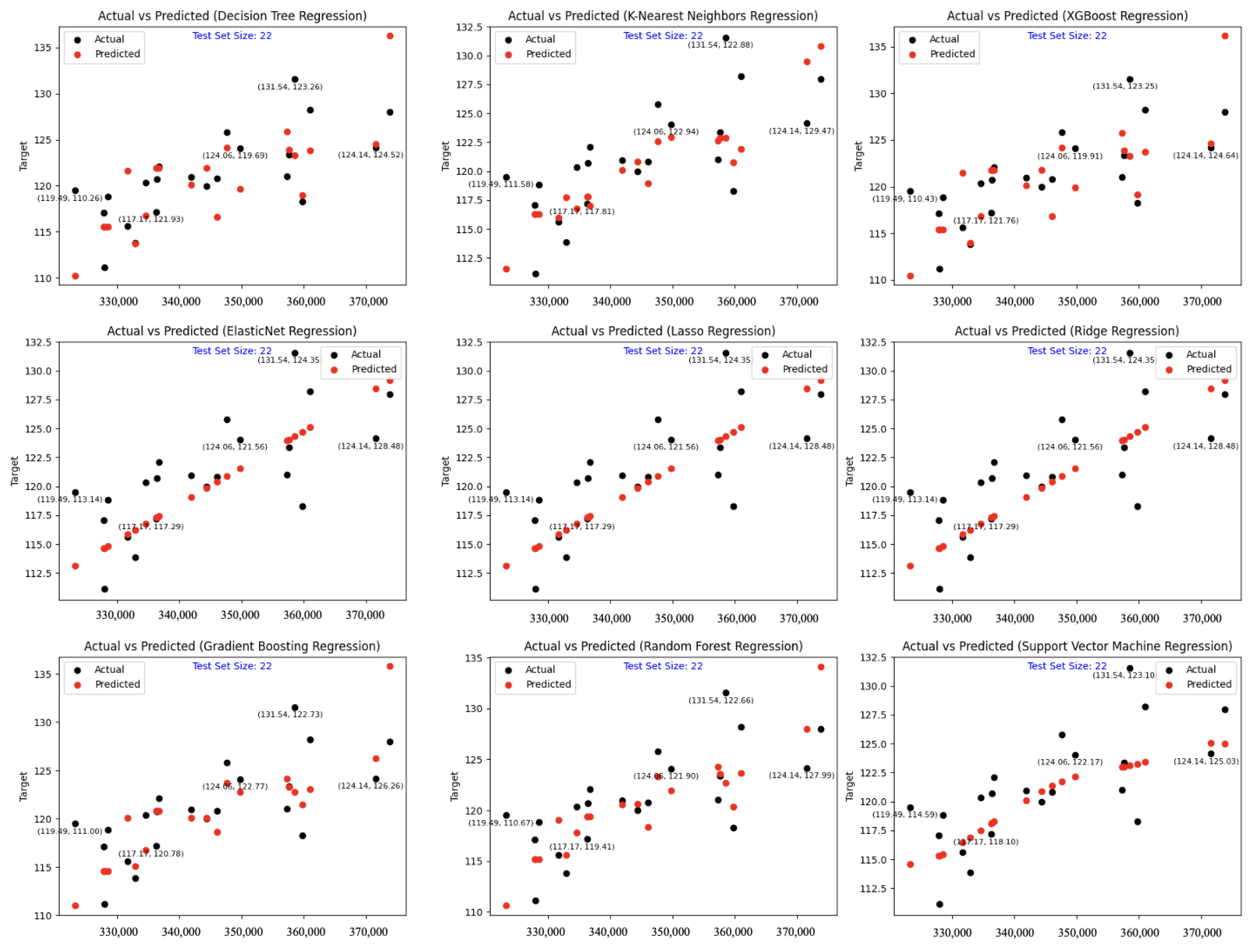
In the results section, we conducted a comparative analysis utilizing various regression models on the same dataset. All models were employed in a supervised learning fashion, where the independent variables (input data) maintained a one-to-one relationship with the dependent variables (output labels). The compared models encompassed Gradient-Boosting Regressor, Tikhonov Regularization (Ridge Regression), K-Nearest Neighbors Regressor (KNeighbors), Random Forest Regressor, Least Absolute Shrinkage and Selection Operator Regression (LASSO Regression), Decision Tree Regression, ElasticNet Regression, and eXtreme Gradient-Boosting Regression (XGBoost Regression).

3.4. Experimental Settings and Evaluation Metrics

3.4.1. Experimental Setup and Training Process

The hardware configuration utilized for training consisted of an Intel® Xeon® E5-2620 v4 @ 2.10 GHz processor (Santa Clara, CA, USA), 64 GB of RAM, and an NVIDIA GeForce RTX 3080 graphics card (Santa Clara, CA, USA). The software configuration included the Windows Server 2019 Server Standard operating system, Python version 3.9.7, CUDA version 11.7, and the PyTorch 2.0.1 framework. During the training process, all models were trained from scratch without pre-loading training weights. We set many parameters; see

Table 1. Experimental parameter settings.

Training Parameter	Value
Input size	640 × 640
Final learning rate	0.01
Optimizer	SGD
Momentum	0.937
Weight decay	0.0005
Batch size	16
Epoch	100

for details.

3.4.2. Evaluation Metrics

In this study, the experimental evaluation of target detection was based on the verification subset of each dataset, and the indicators were the precision, recall, mean average precision (mAP), and giga floating-point operations per second (GFLOPS) to measure the complexity of the neural network calculation model. The variables TP, TN, FP, and FN represent the quantities of true positive, false positive, true negative, and false negative bounding boxes, respectively, in the detection model’s identification of chicken tibias.

Precision: The percentage of correct predictions in the predicted sample.

$$Percision=\frac{TP}{TP+FP}$$

(5)

Recall: The number of correct predictions as a proportion of the total number of positive samples.

$$Recall=\frac{TP}{TP+FN}$$

(6)

Intersection over union (IoU): The ratio of the intersection to the union between a predicted bounding box and a ground-truth bounding box; this is used to quantify their degree of overlap.

$$IoU=\frac{AreaofIntersection}{AreaofUnion}$$

(7)

Mean average precision (mAP): This metric was utilized to evaluate the detection performance of tibia-containing facets of the model. To ensure a comprehensive assessment, it was not appropriate to rely on a single confidence threshold for AP verification. Hence, we employed a range of intersection-over-union (IoU) thresholds to calculate multiple AP values and subsequently averaged them out. Given that this task involved detecting a single category, N = 1.

$$mAP=\frac{1}{N}{\sum }_{i=1}^N{\int }_0^1{P}_i\left(R_i\right)d\left(R_i\right)$$

(8)

$mA{P}_{0.5}$ represents the AP at an IoU threshold of 0.5 and $mA{P}_{0.5:0.95}$ represents the average AP achieved across various IoU thresholds ranging from 0.5 to 0.95 in increments of 0.05.

Mean Absolute Error (MAE): The average of the absolute differences between the true and predicted tibia length values. Used to measure the average of the residuals in the dataset.

$$MAE=\frac{1}{N}\sum _{i=1}^N\left|\widehat{y_i}-y_i\right|$$

(9)

Mean Squared Error (MSE): Represents the mean of the absolute difference between the true tibia length value and the predicted tibia length value in the regression model.

$$MSE=\frac{1}{N}\sum _{i=1}^N{\left(\widehat{y_i}-y_i\right)}^2$$

(10)

Root Mean Square Error (RMSE): Refers to the square root of the mean square error (MSE), which is used to measure the standard deviation of the residuals.

$$RMSE=\sqrt{\frac{1}{N}\sum _{i=1}^N{\left(\widehat{y_i}-y_i\right)}^2}$$

(11)

4. Experimental Results and Analyses

4.1. Ablation Experiments

In order to verify the improved performance of the model, ablation experiments were performed on combinations of various components, which were then tested on the tibia dataset. The average precision (AP) metric was utilized to evaluate the detection performance of tibia-containing facets of the model. mAP@[0.5, 0.95] represents the average AP achieved across various IoU thresholds ranging from 0.5 to 0.95 in increments of 0.05. The results of the ablation experiments are shown in

Table 2. The results of the ablation experiments.

Backbone	EMA	ParNet	CARAFE	WIoU	${\mathit{mAP}}_{0.5:0.95}$ (%)
C2F					86.7
C2F	✓				89.7
C2F	✓	✓			89.9
C2F	✓	✓	✓		90.1
C2F	✓	✓	✓	✓	90.8

.

4.2. Comparative Experiments with Tibia-YOLO

There were changes in both the parameter quantity and mAP. It can be observed in

Table 3. Comparison of different modules at the end of the Backbone.

Model	Parameters/M	GFLOPs	${\mathit{mAP}}_{0.5:0.95}$ (%)
YOLOv8-s	11.2	28.8	86.7
SKAttention	33.3	46.5	90.2
DoubleAttention	11.4	29.0	87.4
MHSA	12.0	29.1	86.6
ParNet	14.1	30.1	89.1

that, based on YOLOv8-s, we improved some terminals of the Backbone and improved the performance of the network by adding the ParNet attention module. It should be noted that, although the average accuracy reached 90.2% after adding the SKAttention module, more parameters were added at the same time, so many computing resources were sacrificed. The number of parameters that we added was 13.12% of the number of parameters added with the SKAttention module, and the average accuracy was very close.

Subsequently, we compared the addition of the same EMA module in front of the three detection heads of the Neck and the addition of other attention modules, and we focused on observing changes in the parameter quantities and mAP. In

Table 4. Comparison of additions of multi-scale attention mechanisms to the Neck.

Model	Parameters/M	GFLOPs	${\mathit{mAP}}_{0.5:0.95}$ (%)
YOLOv8-s	11.2	28.8	86.7
SKAttention× 3	40.2	81.8	90.5
MHSA×3	12.2	30.7	85.5
TripletAttention×3	11.2	29.1	88.7
NAMAttention×3	11.2	28.8	88.2
EMA×3	11.2	29.6	89.7

, we can see the multi-scale attention mechanism’s improvement of the network. Through observation, we found that, after adding EMA modules at different scales, the average accuracy was 3% higher than that of the baseline, but the number of parameters basically did not change, ensuring the operating efficiency of the deep network.

In order to verify the effectiveness of using WIoU, we added a variety of loss functions for comparison after adding the ParNet module and EMA module to YOLOv8-s and using the CARAFE upsampling operator. As can be seen in

Table 5. Comparison of the use of different loss functions.

Loss Function	${\mathit{mAP}}_{0.5:0.95}$ (%)
YOLOv8s + ParNet + EMA + CARAFE (BaseLine)	90.1
BaseLine + CIoU	90.1
BaseLine + DIOU	90
BaseLine + EIOU	90.5
BaseLine + GIOU	90.4
BaseLine + WIOU	90.8

, after comparing Complete-IoU (CIoU) [41], Distance-IoU (DIoU) [41], Efficient-IoU (EIoU) [42], Generalized-IoU (GIoU) [43], and Wise-IoU (WIoU), it was finally found that the WIoU loss function was very advantageous in improving the accuracy. Although 0.1 GFLOPS was added, the mAP accuracy was improved by 0.7%.

We compared the improved Tibia-YOLO model based on YOLOv8-s with representative advanced models for other target detection tasks on the Tibia dataset, and we evaluated the changes in parameter size ($mA{P}_{0.5:0.95}$).

Table 6. Comparison of different network models on the Tibia dataset.

Model	${\mathit{mAP}}_{0.5:0.95}$ (%)
YOLOX	18.6
Fast R-CNN	31.1
YOLOv7	48.7
YOLOv4-tiny	52.3
Faster R-CNN	61.9
RetinaNet	71.0
SSD	71.5
YOLOv5	82.1
YOLOv8-s	84.7
Tibia-YOLO	90.8

shows a comparison of different network models on the Tibia dataset. In Figure 7, the results of running different models are analyzed. The Tibia-YOLO model had the highest detection accuracy and confidence, followed by the YOLOv8-s model. The confidence of the YOLOv5 and SSD models decreased. Although the $mA{P}_{0.5:0.95}$ values of the SSD and RetinaNet models were very close, the test results of the RetinaNet model generated incorrect detection frames. After the analysis, the RetinaNet model used focal loss to deal with the problem of an imbalance between positive and negative samples, but this processing method was not applicable to our Tibia dataset, as it would result in false detection. The performance results of YOLOv7, Fast R-CNN, and YOLOX were not good. The results for $mA{P}_{0.5:0.95}$ did not reach 50%, and it can be seen in the figure that these three target detection models produced a large number of false detections and omissions. From the current point of view, Tibia-YOLO had the best performance in the test on the Tibia dataset.

Finally, our model was tested on two public datasets. The two public datasets were the VOC2012 target detection dataset and the COCO2016 target detection dataset. In this test, we focused on YOLOv8-s. The performance improvements of the baseline and improved TB-YOLO included improvements in the $mA{P}_{0.5}$ and $mA{P}_{0.5:0.95}$ parameters. As in Figure 8,

Table 7. The performance of Tibia-YOLO on three datasets, and the comparison with the basic YOLOv8-s as the baseline.

Model	VOC2012 Dataset		COCO2016 Dataset		Tibia Dataset
	${\mathit{mAP}}_{\mathbf{0.5}}$(%)	${\mathit{mAP}}_{\mathbf{0.5}\mathbf{:}\mathbf{0.95}}$(%)	${\mathit{mAP}}_{\mathbf{0.5}}$(%)	${\mathit{mAP}}_{\mathbf{0.5}\mathbf{:}\mathbf{0.95}}$(%)	${\mathit{mAP}}_{\mathbf{0.5}}$(%)	${\mathit{mAP}}_{\mathbf{0.5}\mathbf{:}\mathbf{0.95}}$(%)
YOLOv8-s	62.0	44.9	57.1	41.4	99.5	84.7
Tibia-YOLO	62.6	45.9	58.3	42.6	99.5	90.8

shows the performance of TB-YOLO on three datasets, as well as a comparison with the basic YOLOv8s as the baseline. As can be seen in the table, the performance of our model on the public COCO2016 and VOC2012 datasets improved, but the improvements in the $mA{P}_{0.5}$ and $mA{P}_{0.5:0.95}$ parameters were relatively small, and the test results on the Tibia dataset improved. Notably, $mA{P}_{0.5:0.95}$ increased by 6.1%. We analyzed this phenomenon. This might have occurred because our dataset was a single-category detection task that was relatively simple and more suitable for the TB-YOLO network. In the tests of the COCO2016 and VOC2017 datasets, although there was a certain improvement there were too many categories involved. As a result, the improvement was not as large as the improvement on the Tibia dataset. As can be seen in Figure 8, the test results of the improved Tibia-YOLO model on the three datasets improved in comparison with those of YOLOv8-s (baseline). In a test on the COCO2016 dataset, it could be seen that Tibia-YOLO could recognize people in the distance and had good small-target detection capabilities.

4.3. Experimental Comparison of Regression Models

We extracted the number of pixels of the height of the detection frame and used the support vector regression (SVR) method for regression. In the regression problem, our independent variable was the number of pixels in the detection frame, which was usually around 350,000, and the dependent variable was the length of the tibia in millimeters, which was usually around 120 mm.

In

Table 8. Comparison of the errors of different regression models.

Model	MAE (mm)	MSE (mm2)	RMSE (mm)
Decision Tree	3.10	16.14	4.35
XGBoost	3.36	18.34	4.28
Gradient Boosting	3.17	16.25	4.03
KNeighbors	3.20	15.34	3.91
RandomForest	3.16	15.06	3.88
LASSO Regression	3.02	13.31	3.65
Ridge Regression	3.02	13.31	3.65
ElasticNet	3.02	13.31	3.65
SVR	2.77	11.39	3.37

, we compare the evaluation indicators of nine regression models: GradientBoosting Regressor, Ridge Regression, KNeighbors Regressor, RandomForest Regressor, LASSO Regression, Decision Tree Regression, ElasticNet Regression, XGBoost Regression, and SVR. It was observed from the regression data that the independent variables were all relatively large numbers, while the dependent variables were relatively small. This indicated that our data involved a high-dimensional input space. SVR proved to be more adaptable in a high-dimensional space and handled large independent variables effectively. Simultaneously, the kernel technique of the SVR model was better adapted to nonlinear relationships. Furthermore, SVR was more robust to outliers and noise, which is crucial with high-dimensional data. We analyzed the KNeighbors Regressor method and found that the computational cost of this method was too high when processing high-dimensional data, and it was abnormally sensitive to noise and outlier values. Two methods, Gradient-Boosting Regressor and Decision Tree Regression, were sensitive to noise and easily caused overfitting.

4.4. Analysis of the Results

Through the comparison of the results in Table 6, it can be seen that our Tibia-YOLO model provided relatively good improvements in comparison with other models. In Figure 7, an example of the detection in some tests is shown, except for the Tibia-YOLO and YOLOv8 models, which produced results that were skewed and did not include the complete tibia in the image. Some of them produced false detection boxes and missing detection boxes, and it turned out that our Tibia-YOLO model performed well in detecting tibias. To test the generalization of the model, we used two public datasets, VOC2012 and COCO2016. As shown by the comparison of the baseline model with YOLOv8 before the improvement and the baseline model with Tibia-YOLO after the improvement—see the test results on the three datasets in Table 7—the detection accuracy improved for each dataset. As can be seen in Figure 8, our Tibia-YOLO model also performed well in the detection of small targets. Our proposed Tibia-YOLO model was able to achieve an average accuracy of 90.8% in the task of broiler tibia detection; it had improved performance in tests of its generalization to other datasets, and it had excellent small-target detection abilities. However, the blurring of the boundaries between muscle tissue and skeletal tissue caused by the activity of broilers during DR image collection will lead to a reduction in the robustness of the application in real-life scenarios. The limitation of the current method is that it only applies to broiler chickens, and its effectiveness for other poultry animals such as ducks and rabbits has not been confirmed. Additional validation and adjustment will be required when generalizing the model to other poultry species.

In Figure 9, a scatter plot is used to depict the predicted results and true values for nine regression models. It was observed that the prediction results of LASSO Regression, ElasticNet, and Ridge Regression were evenly distributed on a straight line. Although this situation demonstrated a better fitting effect on the scatter plot, to ensure the robustness and generalization ability of the models a comprehensive evaluation of model performance using indicators such as the mean square error and mean absolute error was still necessary. By comparing the MAE and RMSE in Table 8, it was found that their results were very similar, differing only by a few decimal places. The main differences among LASSO, ElasticNet, and Ridge Regression were their regularization terms. However, if the same features were chosen for these models to fit a given problem, their predictions could also have been very similar. Through the analysis of the results presented in Table 8, it was determined that SVR was more practical for complex nonlinear problems, and for large high-dimensional data such as pixels, the SVR regression method performed better. Among the 22 sets of test data that were not used for training at all, the mean absolute error (MAE) and root mean square error (RMSE) were 2.77 mm and 3.37 mm, respectively. As shown by the combination of the scatter point distribution and the comparison of the MAE, MSE, and RMSE, SVR performed well in all aspects. It was also proven that the system could accurately measure the tibia length and could be used to detect leg diseases in broiler chickens for breeding.

5. Conclusions

In this study, to solve the problem of the difficulty of detecting leg diseases in broiler chickens, we proposed a system for assisting in measuring the length of the tibia in broilers’ legs. By observing changes in tibia length in real time, leg diseases in broiler chickens can be eliminated and prevented. In order to save effective computing resources in practical applications, we did not introduce too many parameters. We used the CARAFE upsampling operator, integrated a parallel network attention mechanism (ParNetAttention) into the Backbone, and incorporated the efficient multi-scale attention mechanism into multiple channels within the Neck. We proposed the Tibia-YOLO tibia detection model, which was combined with a subsequent SVR regression model to measure the length. Tests showed that, on the Tibia dataset, $mA{P}_{0.5:0.95}$ increased by 6.1%. It increased on both the VOC2012 and COCO datasets, and the improved model did not cause too much of an increase in the number of parameters and GFLOPS. In the regression model that was fitted using the test results, the mean square error (MAE) and root mean square error (RMSE) were 2.77 mm and 3.37 mm, respectively. The performance was very good, and the tibia length of live broilers could be accurately measured. This can help the broiler chicken breeding industry detect the occurrence of broiler leg diseases more efficiently. Compared with the traditional measurement method that uses vernier calipers after dissection or a tape measure in vivo, our method improved the measurement accuracy and efficiency and could better protect broilers. Although the performance of the Tibia-YOLO model was good, there were some unexpected problems in the test set of the Tibia dataset. Certain broilers exhibited increased activity during DR image capture, resulting in instances of edge blurring in the captured images. In such cases, the Tibia-YOLO model struggled to accurately discern the positional relationships of tibias, leading to imprecise bounding box detection. This, in turn, affected subsequent length prediction tasks, necessitating an enhancement in the detection accuracy of the Tibia-YOLO model. Acknowledging the limitations of the approach, we endeavored to diversify the broiler selection as much as possible during the establishment of the Tibia dataset. This involved capturing images of broilers from various breeds, ages, and weights to augment the model’s generalization capabilities. Presently, the method has not been widely adopted for measuring other parts of broilers. Furthermore, it has not gained popularity for application to other poultry species, such as ducks and rabbits. Future endeavors in this work will require the incorporation of a broader spectrum of poultry categories and diverse anatomical detection sites, paving the way for more advanced auxiliary detection technologies in poultry breeding facilities.