Design and Analysis of Yoshimura Tubular Origami Mechanisms

Abstract

The Yoshimura tubular origami mechanism possesses numerous advantageous properties and, when integrated with advanced material technologies, can be applied across various engineering disciplines. However, current research on Yoshimura origami predominantly focuses on centrally symmetric tubular origami mechanisms, which restricts the structural forms and motion patterns of these mechanisms. Drawing inspiration from the biological concept of “morphological variation,” we propose a novel tubular origami mechanism based on the Yoshimura pattern, which is the main contribution of this research. We analyze the Yoshimura planar crease elements and introduce both heterocellular and homocellular tubular origami mechanisms. Furthermore, we establish the origami topology matrices for the Yoshimura tubular origami mechanisms. This research also investigates complex motion forms that differ from traditional Yoshimura origami mechanisms, including macroscopic twisting and compound movements, thereby providing an intuitive design approach and extensive structural guidance for research in Yoshimura tubular origami engineering. Based on the tubular origami mechanism, we created an origami robot and investigate its motion characteristics.

1. Introduction

Origami mechanisms, with their unique properties, such as reconfigurability, negative Poisson’s ratio, and high deployable ratio [1,2,3,4,5], have been widely applied in various fields, including aerospace [6,7], biomedical engineering [8,9], origami robotics [10,11,12,13,14,15], architectural and civil engineering [16,17], and spatially deployable mechanisms [6,18]. The ongoing advancement of mathematical fields, such as computer science, graph theory, and computational geometry, has further bridged the art and science of origami through mathematical principles. For example, foldable space structures based on origami principles enable the creation of lightweight, compact, and expandable designs that can be efficiently deployed in space applications. These structures leverage origami’s compactness and reconfigurability to improve deployment efficiency while reducing spatial constraints during launches. Additionally, integrating soft materials with origami structures has enhanced mobility and introduced novel movement patterns. Haoyong Yu [19] developed an amphibious origami robot with multimodal locomotion and body sensing capabilities, allowing for seamless transitions between land and water. This innovation holds promise for applications in environmental monitoring, search and rescue, and exploration. Tao Jin [20] proposed an origami-inspired soft actuator that integrates stimulus perception and crawling capabilities, enabling robots to sense environmental changes and respond dynamically, demonstrating potential for adaptive, untethered applications in exploration and environmental monitoring. An origami-based soft robotic gripper was also introduced, utilizing a water-bomb design with silicone and latex materials. This gripper achieves versatile, gentle handling of fragile objects through negative pressure actuation, making it suitable for a variety of applications [21]. Inspired by the rhombic dodecahedron (RDD) origami model, Fuwen Hu [22] introduces a 3D-printed soft multicellular robot with multimodal locomotion, including crawling, turning, and climbing. Its reconfigurable design enables diverse patterns and functions without reshaping. Junfeng He [23] introduced a Miura-derived origami tube with programmable stiffness for a modular continuous robot. This robot, driven by steel wires, exhibits flexibility, scalability, and kinematic adaptability, as demonstrated in prototype experiments. Kirigami [24], a related art form that combines cutting and folding, has also been employed to design mechanisms with broader motion and transformation capabilities, expanding the versatility of origami-based engineering solutions. By precisely controlling the folding and unfolding of origami units, engineers can dynamically adjust mechanical properties such as stiffness and damping [25]. Researchers have also explored origami mechanisms with negative Poisson’s ratios for applications in morphing structures, energy absorption, and deployable systems. Recent studies have optimized these structures to enhance their elasticity and deformation behavior [26].

Among various origami mechanisms, Yoshimura tubular origami stands out as one of the most popular. The three-dimensional Yoshimura tubular origami mechanism is typically centrally symmetric. Most research has focused on such symmetric Yoshimura tubes, often achieving specific functions through crease optimization [27], structural modification [28], and the integration of new materials [29,30]. For example, Hongliang Ren [31] and colleagues developed an origami-based mobile robot structure utilizing a Yoshimura mechanism for axial crawling and obstacle navigation. George M. Whitesides [32] introduced a manufacturing method for a soft pneumatic actuator using elastomers embedded with non-expandable thin-walled or fiber structures, enabling anisotropic movements under pneumatic input. Similarly, Xianhe Wei [33] proposed a high-elongation origami robot based on the cutting principle, identifying factors limiting axial elongation and proposing a method to eliminate the negative Poisson’s ratio by reducing material, thus improving the compliant axial elongation of Yoshimura tubular mechanisms. However, existing research predominantly relies on centrally symmetric Yoshimura tubular origami mechanisms. This singular structural form limits their structural and motion diversity, thereby constraining their applications. Expanding research to include asymmetrical and unconventional designs could unlock new functionalities and broaden the potential of Yoshimura tubular origami in engineering.

Research on metamorphic mechanisms dates back to a 1995 study involving gift-wrapping paper boxes [34]. Essentially, metamorphic mechanisms have their roots in the ancient art of origami. In 1998, Professor Jiansheng Dai and Rees Jones introduced the concept of “metamorphic mechanisms” [35] and, in 2005, proposed a topological matrix representation method for these mechanisms [36]. These foundational studies offered a feasible design framework for origami mechanisms.

Building on the principles of metamorphic mechanisms, this paper presents a Yoshimura tubular origami mechanism and establishes the corresponding origami topology matrix. The objective is to enhance the structural and motion diversity of Yoshimura tubular origami mechanisms, offering designers a more intuitive design approach.

The contributions of this work are summarized as follows: (1) Inspired by the biological concept of “cell transformation,” we introduce a novel tubular-based origami mechanism derived from the Yoshimura pattern, broadening the application scope of the Yoshimura origami concept. (2) We investigate various crease configurations, including left-biased and right-biased designs, which enable the development of both heteromorphic (different-shaped) and homomorphic (similar-shaped) origami structures, thereby enhancing the diversity of origami design. (3) We explore complex motions in Yoshimura origami that have been largely overlooked, such as macroscopic twisting movements and compound motions. This investigation provides new perspectives on the potential applications and dynamic capabilities of origami structures.

The paper is structured as follows: Section 2 analyzes the planar crease shape elements of the Yoshimura pattern and proposes a tubular origami mechanism based on this pattern. Section 3 introduces a topological matrix representation method for the proposed Yoshimura tubular origami mechanism, referred to as the origami topology matrix, and validates it with a specific example. Section 4 explores complex motion forms that differ from traditional centrally symmetric Yoshimura tubular origami mechanisms. 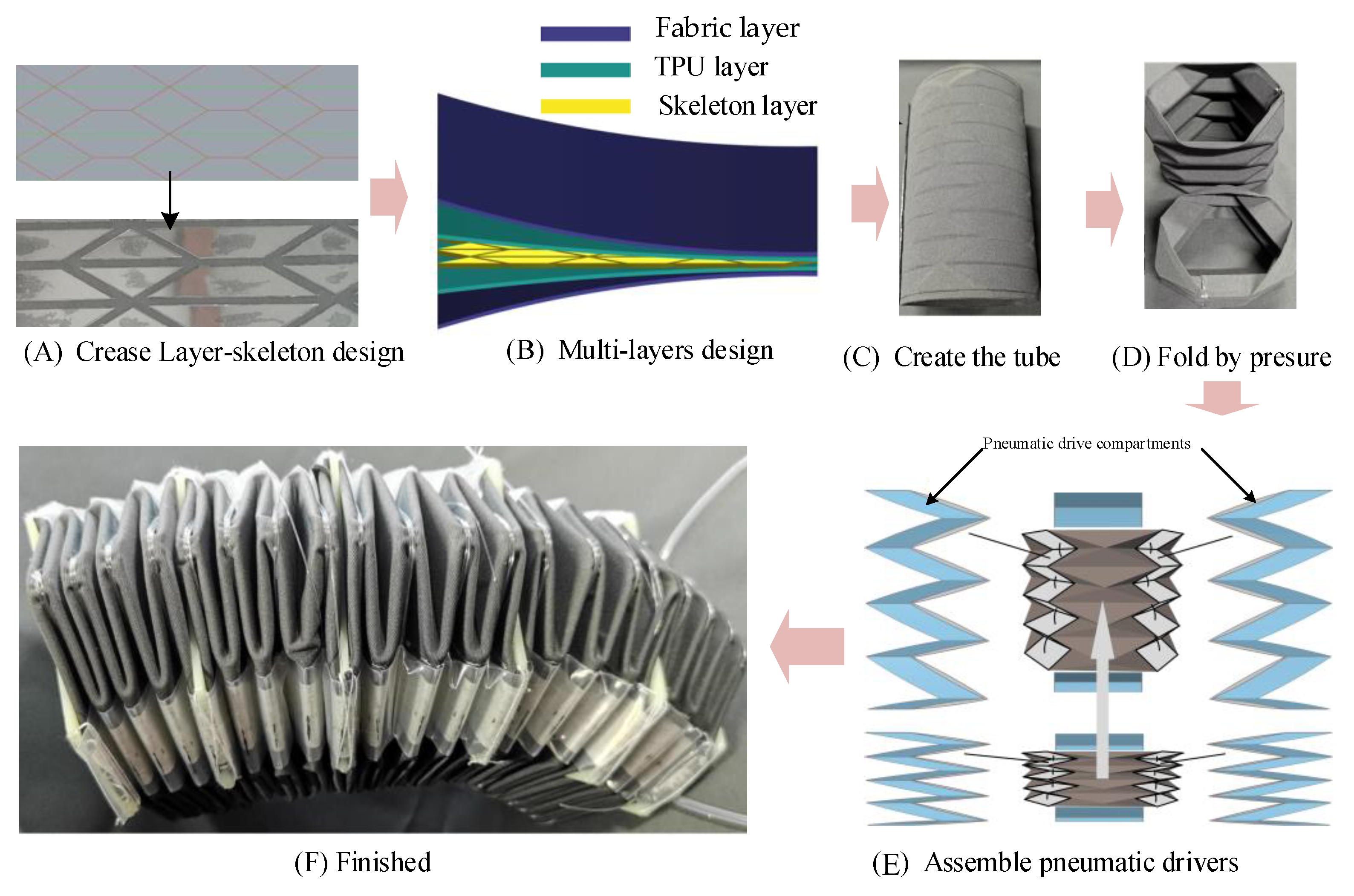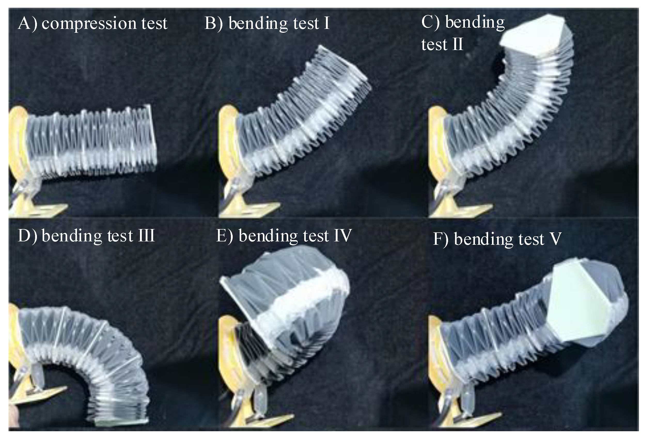In Section 5, the method of making an origami robot is presented and its motion characteristics are analyzed. Finally, Section 6 and Section 7 present the discussions and conclusions, respectively.

2. Mechanism Analysis of Yoshimura Tubular Origami

2.1. Crease Shape Elements

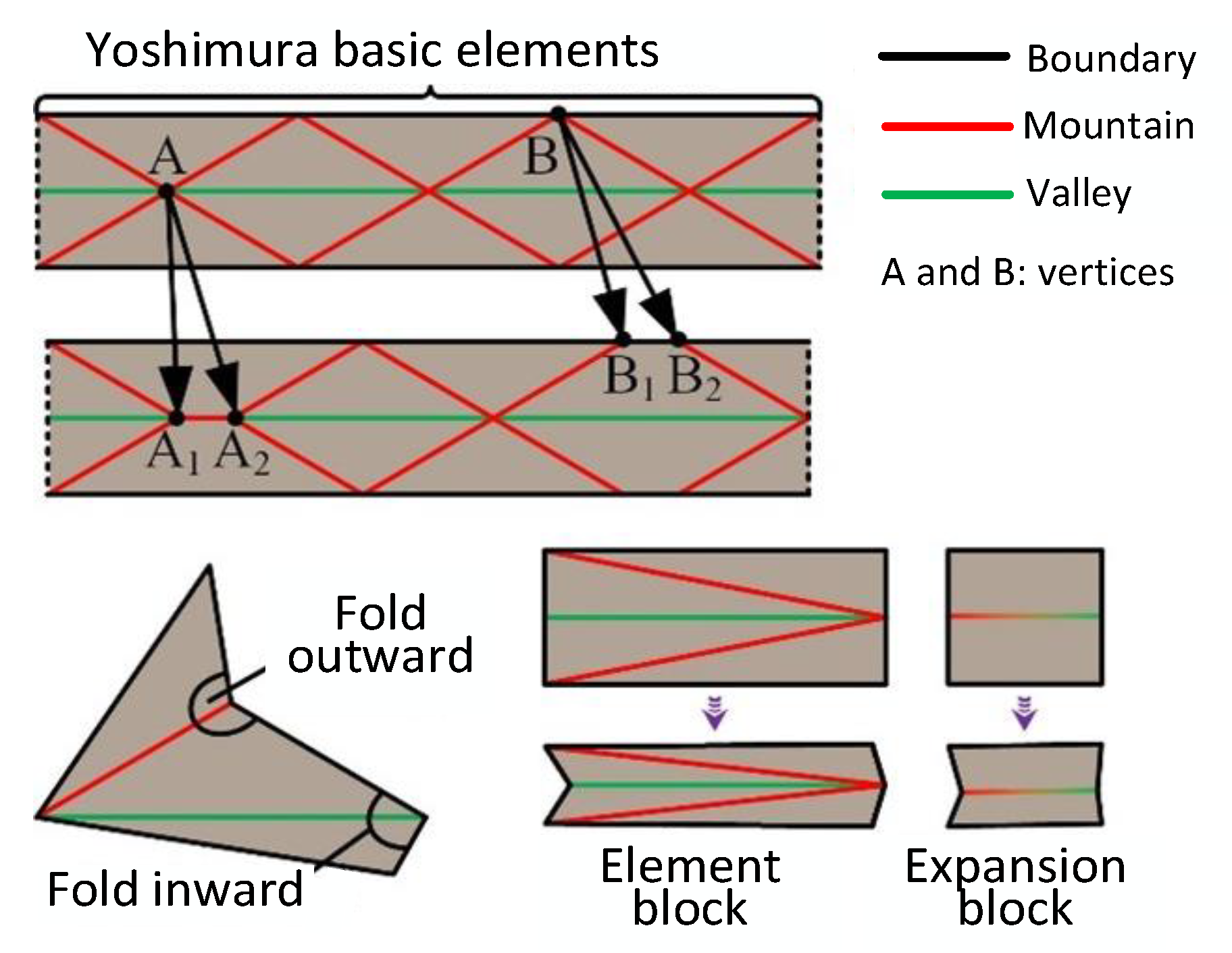
The Yoshimura two-dimensional crease pattern is composed of element blocks and expansion blocks, which are named after commonly used components in the field of Yoshimura origami, as shown in Figure 1. These two types of blocks can be repeatedly folded outward or inward, along mountain lines or valley lines. This paper focuses on exploring the most common six-element Yoshimura origami mechanism.

As shown in Figure 2, for a typical Yoshimura origami mechanism with a bivariate planar crease pattern, the crease’s boundary lines can be joined end-to-end to form a cylindrical tube shape. When this cylindrical shape is folded along its original crease patterns, mountain lines and valley lines, a Yoshimura tubular origami mechanism is formed. Planar creases are usually composed of a repeating arrangement of crease elements and, when folded into a cylindrical shape, the crease shape elements at both ends appear separated on the planar crease. This study focuses on analyzing a complete set of crease shape elements highlighted within a defined boundary.

The external boundary lines and the internal mountain lines of the selected set of crease shape elements are symmetrically aligned with respect to the central valley line. To better observe the characteristics, we define the crease shape elements so that the valley line is positioned at the bottom and the mountain line at the top. A perpendicular bisector is drawn from the lower valley line, and a perpendicular line is drawn down to the lower valley line from the peak of the upper mountain line. The two types of crease shape elements are defined as follows:

The crease shape element is defined as a left-biased crease shape element if the perpendicular from the peak of the mountain line to the valley line falls on the left side of the perpendicular bisector of the valley line.

The crease shape element is defined as a right-biased crease shape element if the perpendicular from the mountain line’s peak to the valley line falls on the right side of the valley line’s perpendicular bisector.

Since planar creases are often composed of repeated patterns, the boundary line of each group may also serve as the valley line for another group. More generally, in the definitions provided above, the valley line can also be the boundary line.

2.2. Origami Mechanism Derived from Heterocellular Tube

For a single set of planar creases, a tubular origami mechanism folded from different types of crease shape elements is referred to as an origami mechanism derived from a heterocellular tube.

Excluding the expansion blocks, a Yoshimura origami mechanism’s planar creases consist of three types of crease shape elements: standard crease shape elements, left-biased crease shape elements, and right-biased crease shape elements. These correspond to the spatial forms formed after folding: standard cells, left-biased cells, and right-biased cells, respectively. By removing the constraints on the crease width and the crease length of the element blocks in a single set of planar creases and applying the basic principles of permutation and combination, it can be concluded that there are, in a broad sense, three manifestations of origami mechanisms based on heterocellular tubes.

As shown in Figure 3, the planar creases of the standard-left-biased heterocellular tubular origami mechanism are formed by splicing the left-biased crease shape elements in the upper part with the standard crease shape elements in the lower part. It can be observed that the crease shape elements at the left and right ends are not fully intact. To better represent each crease shape element within the planar creases and to retain as much of the complete crease shape elements as possible, the ends of the crease shape elements are intentionally disrupted. However, in the folded spatial form, the crease shape elements remain undamaged. The left-biased and standard cells still manifest with mountain lines corresponding to boundary lines and valley lines, respectively. The combination of standard cells and left-biased cells corresponding to the standard and left-biased crease shape elements forms the standard-left-biased heterocellular tubular origami mechanism.

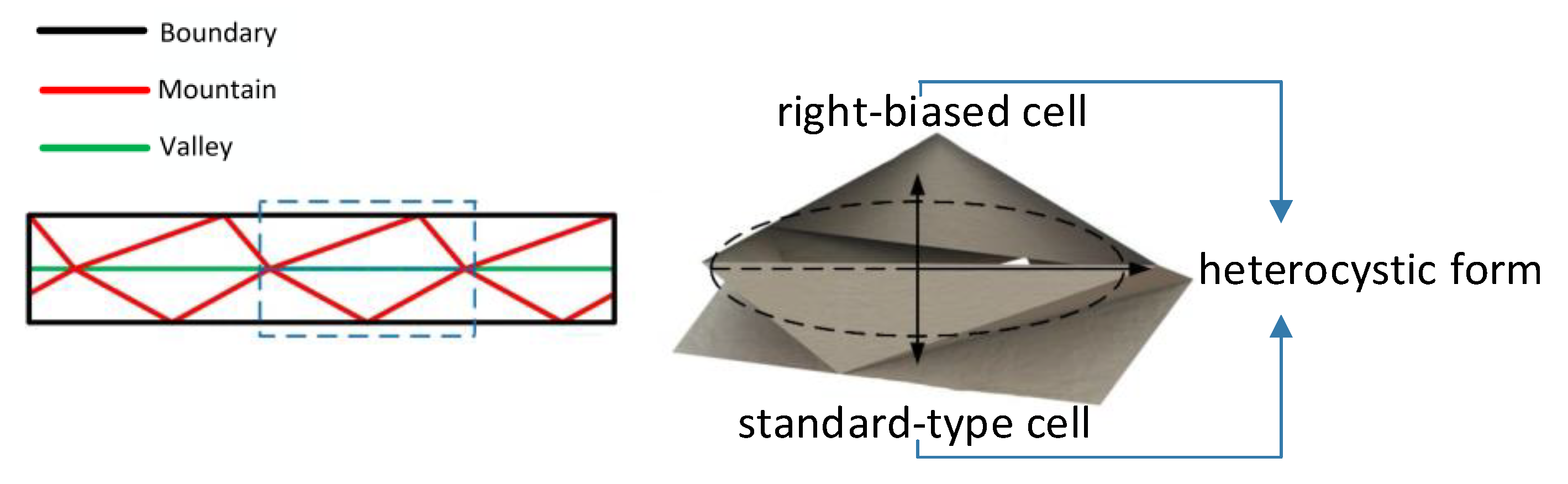
As shown in Figure 4, the planar creases of the standard-right-biased heterocellular tubular origami mechanism are formed by splicing the right-biased crease shape elements in the upper part with the standard crease shape elements in the lower part. The combination of standard cells and right-biased cells corresponding to the standard and right-biased crease shape elements forms the standard-right-biased heterocellular tubular origami mechanism.

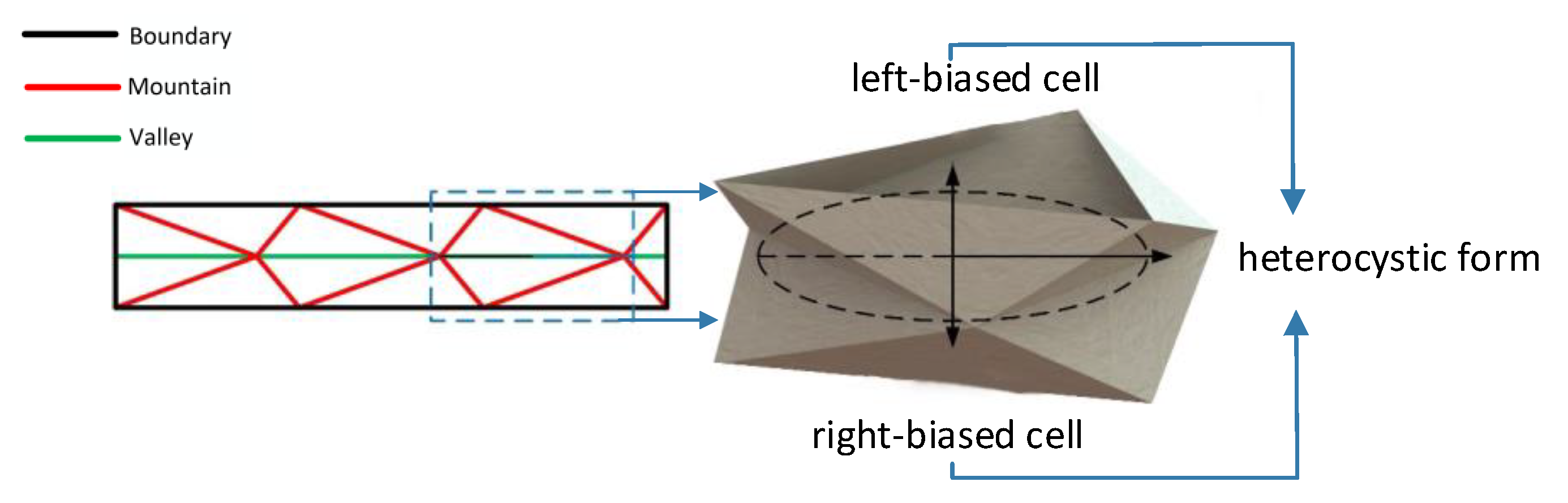
As shown in Figure 5, the planar creases of the left-biased–right-biased heterocellular tubular origami mechanism are formed by splicing the left-biased crease shape elements in the upper part with the right-biased crease shape elements in the lower part. The combination of left-biased cells and right-biased cells corresponding to the left-biased and right-biased crease shape elements forms the left-biased–right-biased heterocellular tubular origami mechanism.

2.3. Origami Mechanism Derived from Homocellular Tube

Similarly, for a single set of planar creases, a tubular origami mechanism folded from identical types of crease shape elements is referred to as a homocellular tubular origami mechanism. The planar creases of the Yoshimura origami mechanism contain the aforementioned three types of crease shape elements, without considering expansion blocks and excluding the constraints of crease width and element block length in a single set of planar creases. In a broad sense, there are three forms of homocellular tubular tube origami mechanisms, as described below.

As shown in Figure 6, the planar creases of the standard-type homocellular tubular origami mechanism are composed of standard crease shape elements. Similarly, the standard cells corresponding to the standard crease shape elements form the standard-type homocellular tubular derivative origami mechanism. This origami mechanism is fully symmetric about its central axis, making it easy to design. The planar creases and the corresponding spatial form are well known and common, as previously analyzed in detail.

As shown in Figure 7, the planar creases of the left-biased homocellular tubular origami mechanism are composed of left-biased crease shape elements. Similarly, the left-biased cells corresponding to the left-biased crease shape elements form the left-biased homocellular tubular derivative origami mechanism.

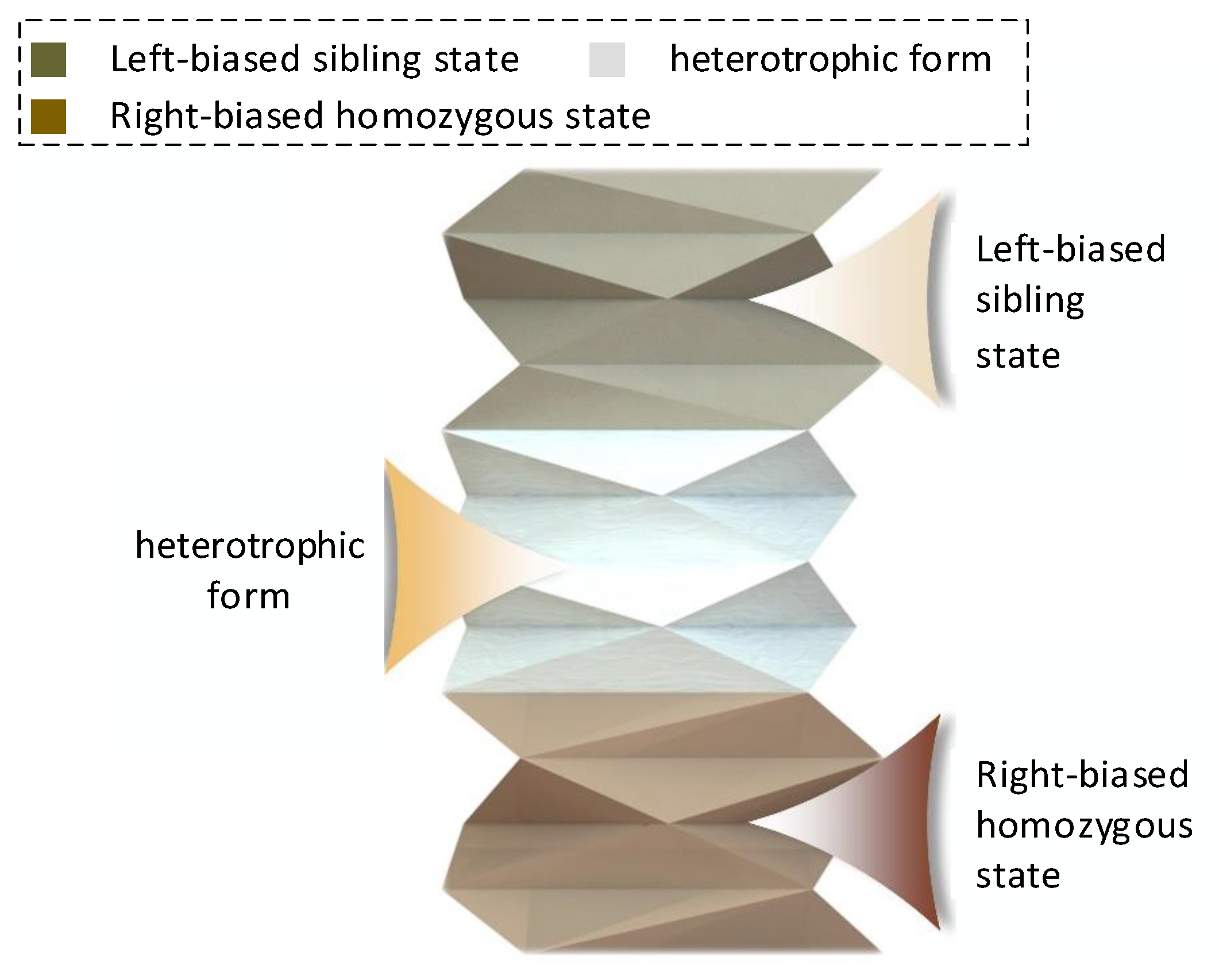
As shown in Figure 8, the planar creases of the right-biased homocellular tubular origami mechanism are composed of right-biased crease shape elements. Similarly, the right-biased cells corresponding to the right-biased crease shape elements form the right-biased homocellular tubular derivative origami mechanism. The external manifestations differ for the heterocellular and homocellular forms of the Yoshimura-type origami mechanisms defined in the above figures, leading to distinct motion characteristics for each mechanism. Depending on the actual requirements, a design can be created that combines both homocellular and heterocellular forms. This section presents an example of such a tubular origami mechanism, as illustrated in Figure 9.

3. The Topological Matrix Representation Method for Yoshimura Origami Configurations

3.1. Description of the Crease Matrix

In the Yoshimura origami planar creases, there are essentially three types of crease shape elements, as shown in Figure 10. The base length $l$ and width $w$ are used to describe the characteristic information of each crease shape element. In addition to the standard crease shape element, an inclination angle $\theta$ is introduced to describe the degree of deviation for the left- and right-biased crease shape elements. As analyzed in Section 3.1, the specific left and right declination angle values are expressed as the magnitude of the angle between the line connecting the vertex of the mountain line to the midpoint of the base and the midsagittal line of the base. It should be noted that, as shown in Figure 10, the base line can correspond to either a boundary line or a valley line.

Thus, the symbol ${\mu }_l^w$ is used to represent the standard crease shape element, ${}^{\nwarrow d}{v}_l^w$, for the left-biased crease shape element, and ${}^{\nearrow d}{o}_l^w$ for the right-biased crease shape element. In these symbols, the subscripts $l$, $w$, and $\theta$ are used to describe the basic characteristic information, including the base length, width, and the left or right inclination angle of the crease shape element.

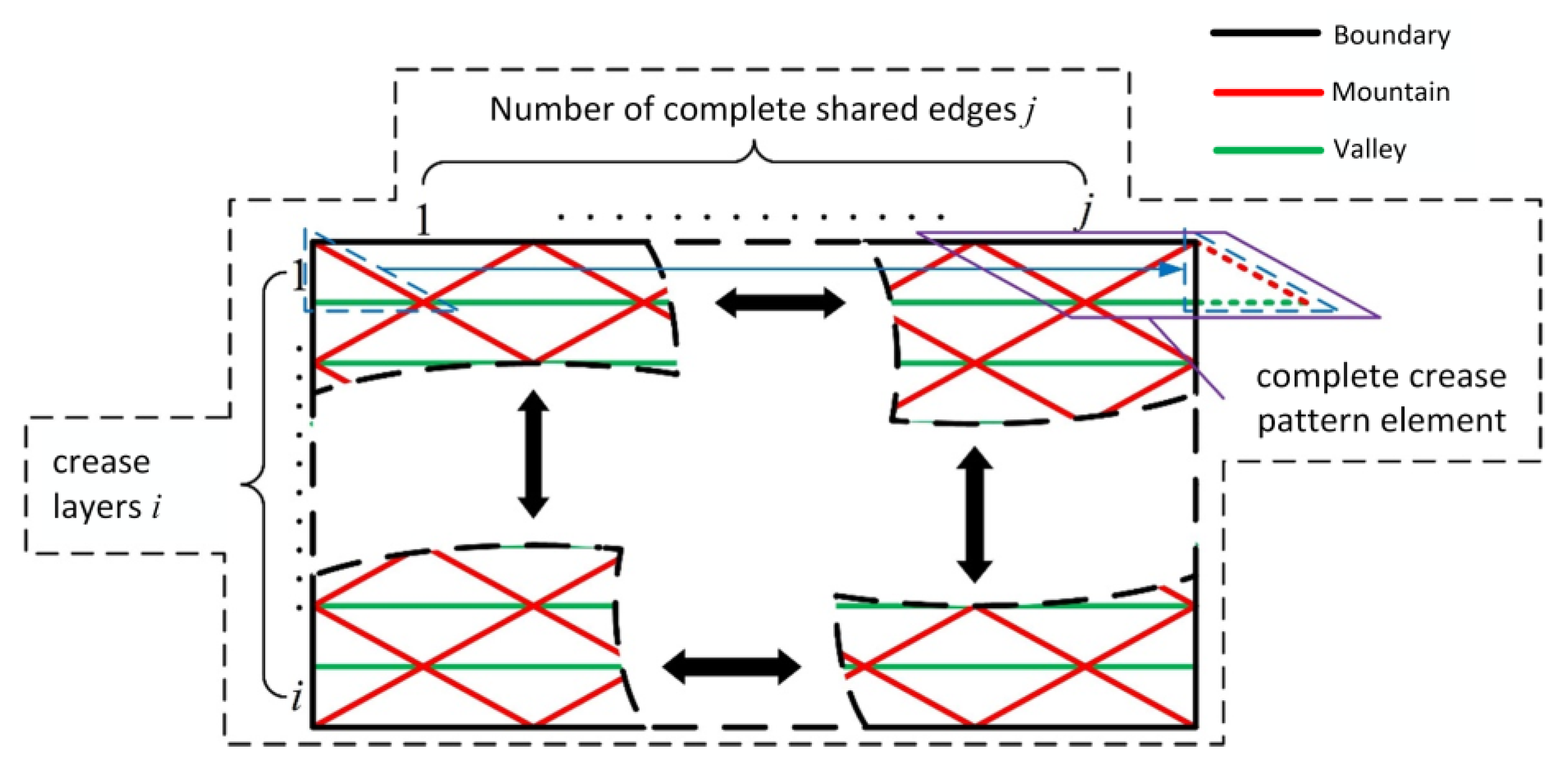
With the symbol representation method for the crease shape elements mentioned above, we can now establish a crease matrix representation method for Yoshimura origami planar creases. The crease matrix is denoted by $\mathbf{M}$, as shown in Equation (1). The following are some explanations regarding the crease matrix $\mathbf{M}$:

$$M=\left[\begin{array}{cccc}{M}_{1,1}& M_{1,2}& \cdots & M_{1,j}\\ M_{2,1}& M_{2,2}& \cdots & M_{2,j}\\ ⋮& ⋮& \ddots & ⋮\\ M_{i,1}& M_{i,2}& \cdots & M_{i,j}\end{array}\right]$$

(1)

As illustrated by the specific meaning of the crease matrix in Figure 11, each element within the crease matrix $\mathbf{M}$ represents the following:

(1) The number of rows $i$ in the crease matrix $\mathbf{M}$ represents the number of layers in the Yoshimura origami planar creases, while the number of columns $j$ represents the number of complete common edges, i.e., boundary lines or valley lines, in each layer of planar creases.

(2) Each element in the rows of the crease matrix $\mathbf{M}$ represents a complete crease shape element within each layer of the planar creases.

(3) Each element in the crease matrix $\mathbf{M}$ can represent different types of crease shape elements, such as the standard crease shape element ${\mu }_l^w$, the left-biased crease shape element ${}^{\nwarrow d}{v}_l^w$, and the right-biased crease shape element ${}^{\nearrow d}{o}_l^w$.

It is important to note that the connection between the layers of planar creases will remain intact only if the length of the boundary lines or valley lines corresponding to each crease shape element is equal. Therefore, it is assumed that the complete common edge length within each layer of planar creases must be equal.

In this section, we introduce the concept of a topological matrix for origami, which enhances our ability to represent and design the spatial form of the Yoshimura origami mechanism. Once the relationship between the plane creases and spatial forms is established, the origami configuration’s topological matrix serves as a more intuitive mathematical tool for representing the designed origami mechanism.

3.2. Description of the Morphological Matrix

In the Yoshimura origami spatial structure, through analysis, there are three types of cells that exist through analysis, standard cells, left-biased cells, and right-biased cells, each composed of corresponding cell elements. The internal constraints of the crease pattern elements corresponding to the cells can result in either a fully overlapped or non-overlapped spatial configuration, which leads to different characteristic information being conveyed even by the same type of cell. In this context, “fully overlapped” refers to the phenomenon where the planes at both axial ends of the cylindrical state can approximately coincide, which is referred to as the fully overlapped spatial configuration of the Yoshimura origami structure. Conversely, the non-overlapped configuration is the opposite of this. Additionally, there may be various cell elements within the cells. Describing the spatial configuration information of such mixed-type cells can be more complex. Given these situations mentioned above, further decomposition for each type of cell is necessary so that resultant cell elements can describe their own spatial configuration information more comprehensively. By decomposing the cells, the characteristic information of each cell element can be described using height $h$. In addition to the standard cell elements, an additional torsion angle $n$ is required to describe the axial torsion of the left-biased and right-biased cell elements.

As shown in Figure 12, the standard cell element can be denoted by the symbol $U$. The fully overlapped standard cell element is denoted by $U_1$, while the non-overlapped standard cell element, which has a certain spatial height, as previously analyzed, is denoted by $U_2^h$.Unlike the standard cell element, the left-biased and right-biased cell elements may not only have spatial height but also a certain axial torsion angle. For the left-biased and right-biased cell elements, the skew angle value of the crease pattern element corresponds to the axial torsion angle in the origami spatial configuration. The determination of the torsion angle and its direction is further explained as follows:

As shown in Figure 13, by taking a cross-sectional view of a cell element from the origami spatial configuration, the left-biased and right-biased cell elements are derived from the standard cell element. Therefore, a hypothetical cross-section corresponding to the standard cell element can be established, represented by the black dashed triangular line. The blue dashed triangular line represents the actual position of the cell element formed after derivation from the standard cell element. The angle formed during the derivation process is defined as the axial torsion angle n of the left-biased and right-biased cell elements. The direction is determined as follows: the left-biased cell element corresponds to a counterclockwise axial torsion angle, while the right-biased cell element corresponds to a clockwise axial torsion angle.

As shown in Figure 14, the left-biased cell element and the right-biased cell element are represented by the symbols $V$ and $O$, respectively. For the left-biased cell element $V$, ${}^{\nwarrow n}{V}_1$ represents the fully overlapped left-biased cell element with a counterclockwise axial torsion angle, and ${}^{\nwarrow n}{V}_2^h$ represents the non-overlapped left-biased cell element with a counterclockwise axial torsion angle. For the right-biased cell element $O$, ${}^{\nearrow n}{O}_1$ represents the fully overlapped right-biased cell element with a clockwise axial torsion angle, and ${}^{\nearrow n}{O}_2^h$ represents the non-overlapped right-biased cell element with a clockwise axial torsion angle.

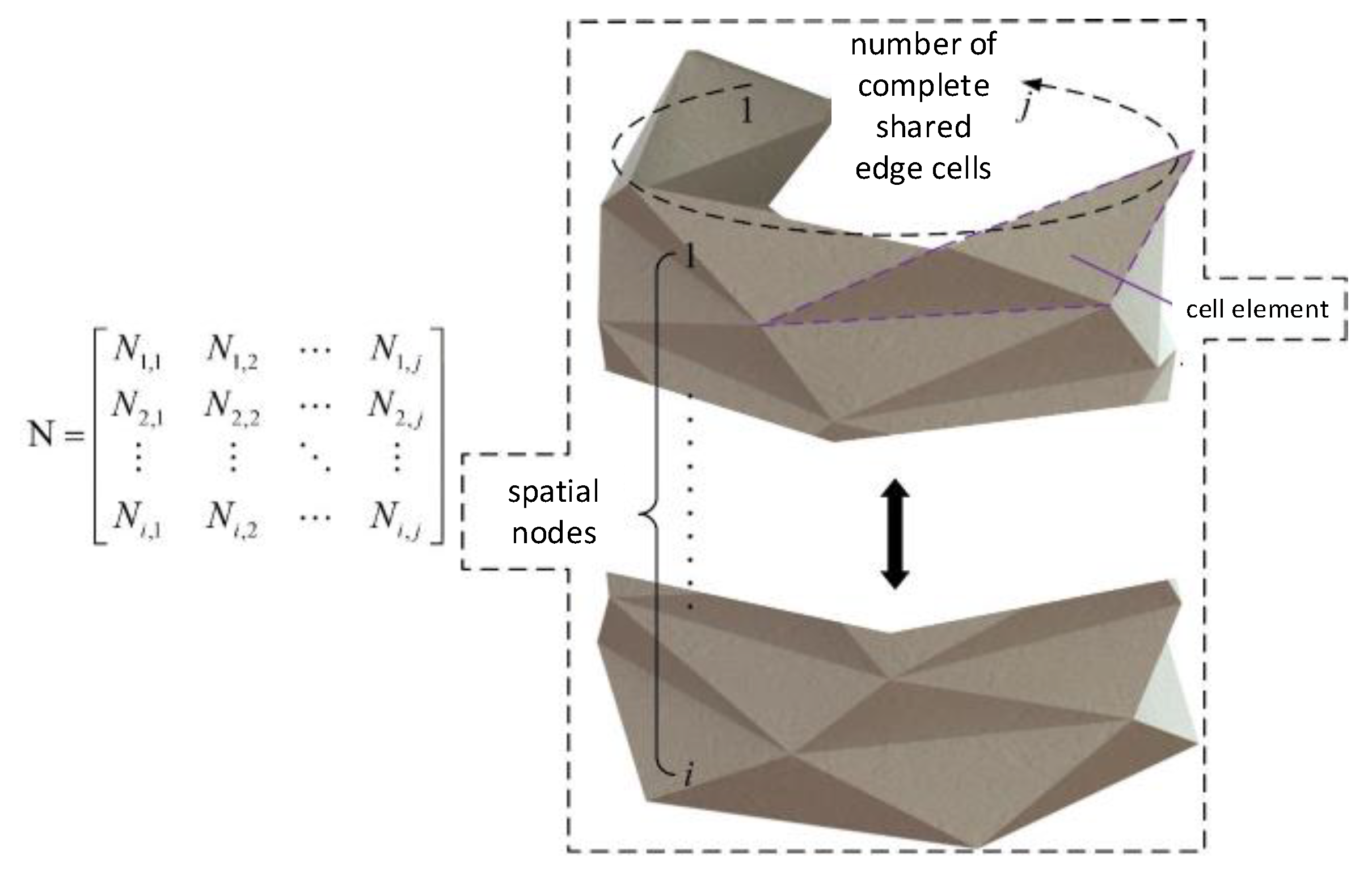
With the symbolic representation of the cell elements established above, we can now develop the method for describing the morphological matrix of the Yoshimura origami spatial structure. The morphological matrix is denoted by $\mathbf{N}$:

$$N=\left[\begin{array}{cccc}{N}_{1,1}& N_{1,2}& \cdots & N_{1,j}\\ N_{2,1}& N_{2,2}& \cdots & N_{2,j}\\ ⋮& ⋮& \ddots & ⋮\\ N_{i,1}& N_{i,2}& \cdots & N_{i,j}\end{array}\right]$$

(2)

and the specific meaning of each element in the matrix $\mathbf{N}$ is as follows:

(1) The number of rows $i$ in the morphological matrix $\mathbf{N}$ represents the number of segments in the Yoshimura origami spatial structure. The number of columns $j$ represents the number of complete common-boundary cells included in each segment of the spatial structure.

(2) The elements in each row of the morphological matrix $\mathbf{N}$ represent the cell elements contained in each segment of the spatial structure.

(3) Each element in the morphological matrix $\mathbf{N}$ can represent different types of cell elements, such as the standard cell element $U_1$ or $U_2^h$, the left-biased cell element ${}^{\nwarrow n}{V}_1$ or ${}^{\nwarrow n}{V}_2^h$, and the right-biased cell element ${}^{\nearrow n}{O}_1$ or ${}^{\nearrow n}{O}_2^h$.

When describing the crease matrix, it is important to note that the assumption of equal complete common boundaries in each layer of the planar crease ensures the folded spatial structure forms a cylindrical closed configuration. Different types of cell elements are generated from the corresponding crease pattern elements in the planar crease. Because the lengths of the crease pattern elements are equal, each segment of the Yoshimura origami spatial structure can be combined. However, since the cell elements formed by the complete crease pattern elements in each row of the crease matrix may or may not be fully overlapped after folding, the overlap condition is related to the length and width constraints within the crease pattern element. Therefore, it is assumed that the overlap condition of each segment of the cell elements must be entirely the same, as illustrated in Figure 15.

3.3. Examples of the Topological Matrix Representations

The above sections have already provided a description of the crease matrix $\mathbf{M}$ and the morphology matrix $\mathbf{N}$. Below, we will present some examples of how to represent Yoshimura origami structures using topological matrices:

$$\left\{\begin{array}{l}l=L\\ {}^{1256}w={\displaystyle \frac{L}{2}}\tan {\displaystyle \frac{\pi }{6}}\\ {}^{34}w={\displaystyle \frac{L}{2}}\end{array}\right.$$

(3)

First, let us represent a standard-type homomorphic tube-derived origami structure. Assume the crease matrix is six rows by three columns; as shown in Equation (3), we initially set the complete common edge length to $L$, and then the base length $l$ of the standard-type crease element can be determined. Regarding the width $w$ of the crease element, as discussed earlier, its value is related to whether the spatial configuration is fully overlapped or not. The superscript of the width of the crease element corresponds to the row number in the crease matrix.

The corresponding crease matrix $\mathbf{M}$ and morphology matrix $\mathbf{N}$ are as follows:

$$\left\{\begin{array}{l}M=\left[\begin{array}{ccc}{\mu }_L^{{\displaystyle \frac{L}{2}}\tan {\displaystyle \frac{\pi }{6}}}& {\mu }_L^{{\displaystyle \frac{L}{2}}\tan {\displaystyle \frac{\pi }{6}}}& {\mu }_L^{{\displaystyle \frac{L}{2}}\tan {\displaystyle \frac{\pi }{6}}}\\ {\mu }_L^{{\displaystyle \frac{L}{2}}\tan {\displaystyle \frac{\pi }{6}}}& {\mu }_L^{{\displaystyle \frac{L}{2}}\tan {\displaystyle \frac{\pi }{6}}}& {\mu }_L^{{\displaystyle \frac{L}{2}}\tan {\displaystyle \frac{\pi }{6}}}\\ {\mu }_L^{{\displaystyle \frac{L}{2}}}& {\mu }_L^{{\displaystyle \frac{L}{2}}}& {\mu }_L^{{\displaystyle \frac{L}{2}}}\\ {\mu }_L^{{\displaystyle \frac{L}{2}}}& {\mu }_L^{{\displaystyle \frac{L}{2}}}& {\mu }_L^{{\displaystyle \frac{L}{2}}}\\ {\mu }_L^{{\displaystyle \frac{L}{2}}\tan {\displaystyle \frac{\pi }{6}}}& {\mu }_L^{{\displaystyle \frac{L}{2}}\tan {\displaystyle \frac{\pi }{6}}}& {\mu }_L^{{\displaystyle \frac{L}{2}}\tan {\displaystyle \frac{\pi }{6}}}\\ {\mu }_L^{{\displaystyle \frac{L}{2}}\tan {\displaystyle \frac{\pi }{6}}}& {\mu }_L^{{\displaystyle \frac{L}{2}}\tan {\displaystyle \frac{\pi }{6}}}& {\mu }_L^{{\displaystyle \frac{L}{2}}\tan {\displaystyle \frac{\pi }{6}}}\end{array}\right]\\ N=\left[\begin{array}{ccc}{U}_1& U_1& U_1\\ U_1& U_1& U_1\\ U_2^h& U_2^h& U_2^h\\ U_2^h& U_2^h& U_2^h\\ U_1& U_1& U_1\\ U_1& U_1& U_1\end{array}\right]\end{array}\right.$$

(4)

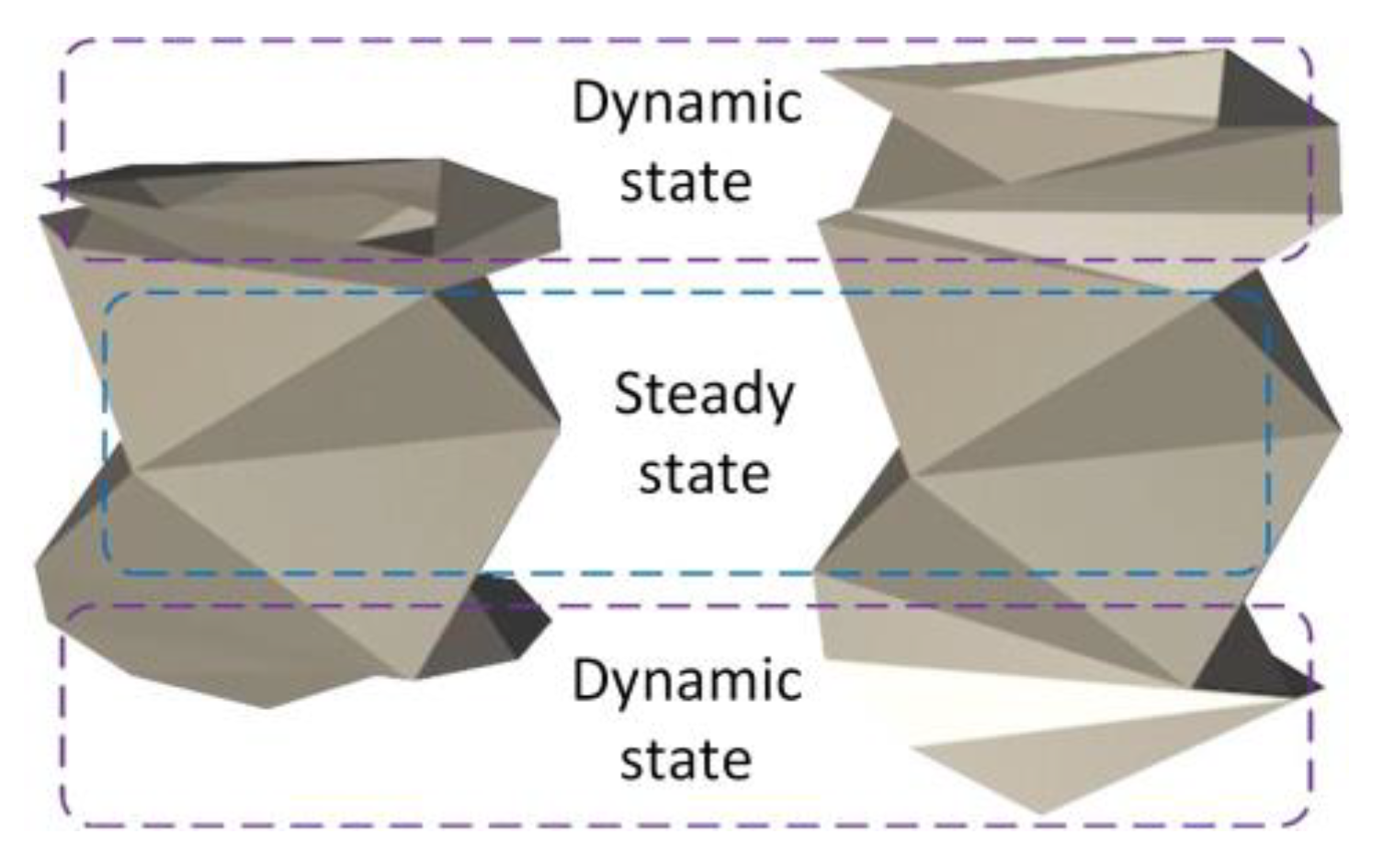
By drawing the spatial configuration, we can observe that, as anticipated in this section, the first, second, fifth, and sixth segments are in a fully overlapped state, while the third and fourth segments are not fully overlapped, as shown in Figure 16. This results in dynamic and stable regions.

Similarly, assume the crease matrix $\mathbf{M}$ is eight rows by three columns. Initially, set the complete common edge length to $L$; then, the base lengths $l$ of the standard-type, left-biased, and right-biased crease elements can be determined. The widths $w$ of the crease elements are related to whether the spatial configuration is fully overlapped or not, and the skewness angle is $d$. The superscript of the width of the crease element corresponds to the row number in the crease matrix, as shown in Equation (5):

$$\left\{\begin{array}{l}l=L\\ {}^{123}w=0.26L\\ {}^{123}d=36.8°\\ {}^{45}w={\displaystyle \frac{L}{2}}\\ {}^{678}w=0.23L\\ {}^{678}d=51.3°\end{array}\right.$$

(5)

The corresponding crease matrix is shown in Equation (6):

$$M=\left[\begin{array}{ccc}{}^{\nwarrow 36.8°}{\nu }_L^{0.26L}& {}^{\nwarrow 36.8°}{\nu }_L^{0.26L}& {}^{\nwarrow 36.8°}{\nu }_L^{0.26L}\\ {}^{\nwarrow 36.8°}{\nu }_L^{0.26L}& {}^{\nwarrow 36.8°}{\nu }_L^{0.26L}& {}^{\nwarrow 36.8°}{\nu }_L^{0.26L}\\ {}^{\nwarrow 36.8°}{\nu }_L^{0.26L}& {}^{\nwarrow 36.8°}{\nu }_L^{0.26L}& {}^{\nwarrow 36.8°}{\nu }_L^{0.26L}\\ {\mu }_L^{{\displaystyle \frac{L}{2}}}& {\mu }_L^{{\displaystyle \frac{L}{2}}}& {\mu }_L^{{\displaystyle \frac{L}{2}}}\\ {\mu }_L^{{\displaystyle \frac{L}{2}}}& {\mu }_L^{{\displaystyle \frac{L}{2}}}& {\mu }_L^{{\displaystyle \frac{L}{2}}}\\ {}^{\nearrow 51.3°}{o}_L^{0.23L}& {}^{\nearrow 51.3°}{o}_L^{0.23L}& {}^{\nearrow 51.3°}{o}_L^{0.23L}\\ {}^{\nearrow 51.3°}{o}_L^{0.23L}& {}^{\nearrow 51.3°}{o}_L^{0.23L}& {}^{\nearrow 51.3°}{o}_L^{0.23L}\\ {}^{\nearrow 51.3°}{o}_L^{0.23L}& {}^{\nearrow 51.3°}{o}_L^{0.23L}& {}^{\nearrow 51.3°}{o}_L^{0.23L}\end{array}\right]$$

(6)

The morphology matrix includes left-biased and right-biased cell elements, both of which can be fully overlapped, and the corresponding skewness angles n can be measured through modeling, as shown in Equation (7):

$$\left\{\begin{array}{l}{}^{123}n=20°\\ {}^{678}n=30°\end{array}\right.$$

(7)

The corresponding morphology matrix $\mathbf{N}$ is then obtained:

$$N=\left[\begin{array}{ccc}{}^{\nwarrow 20°}{V}_1& {}^{\nwarrow 20°}{V}_1& {}^{\nwarrow 20°}{V}_1\\ {}^{\nwarrow 20°}{V}_1& {}^{\nwarrow 20°}{V}_1& {}^{\nwarrow 20°}{V}_1\\ {}^{\nwarrow 20°}{V}_1& {}^{\nwarrow 20°}{V}_1& {}^{\nwarrow 20°}{V}_1\\ U_2^h& U_2^h& U_2^h\\ U_2^h& U_2^h& U_2^h\\ {}^{\nearrow 30°}{O}_1& {}^{\nearrow 30°}{O}_1& {}^{\nearrow 30°}{O}_1\\ {}^{\nearrow 30°}{O}_1& {}^{\nearrow 30°}{O}_1& {}^{\nearrow 30°}{O}_1\\ {}^{\nearrow 30°}{O}_1& {}^{\nearrow 30°}{O}_1& {}^{\nearrow 30°}{O}_1\end{array}\right]$$

(8)

By drawing the spatial configuration, we can observe that, as anticipated, the first, second, third, sixth, seventh, and eighth segments are in a fully overlapped state, while the fourth and fifth segments are not fully overlapped, as shown in Figure 17. This results in dynamic and stable regions.

Through the two examples above, this paper has represented two Yoshimura origami structures using the crease matrix and morphology matrix. In fact, when the planar crease and spatial configuration are correlated, the origami configuration topological matrix can serve as a more intuitive mathematical tool to represent the designed Yoshimura origami structures. On a deeper level, knowing the designed Yoshimura origami structure, it is possible to deduce the corresponding planar crease, providing a theoretical basis for the actual manufacturing of origami structures. This method not only allows for the mathematical representation of origami structures but also offers designers a more intuitive design approach, further aiding the practical production of origami structures.

4. Analysis of the Complex Forms of Movement in the Origami

4.1. Torsion Movements

The telescoping and bending motions in Yoshimura origami structures are well known and widely applied. Typically, these origami structures exhibit a standard symmetrical spatial arrangement. However, the analysis presented in this paper shows that these structures can undergo derivation, leading to a variety of rich spatial configurations with different forms. This observation leads to a hypothesis that the corresponding motion forms of these structures might also change accordingly. A detailed analysis of this possibility is as follows.

Figure 18 and Figure 19, respectively, illustrate the common standard form and the derived skewed form of Yoshimura origami structures, as discussed earlier. In a single-module origami structure, motion can be induced by altering the distance between two opposing faces of the module through a suitable driving mechanism. Essentially, this involves changing the distance between the upper and lower faces of the module, resulting in motion. For a standard-form origami structure, when the distance between the upper and lower faces on one side decreases, a bending motion is induced in the structure, corresponding to a bending angle ${\theta }_b$. In contrast, for the derived skewed form, while a bending angle ${\theta }_b$ also exists, there is an additional difference: after derivation, misalignment occurs between originally aligned circumferential upper and lower faces on one side. This misalignment corresponds to a twist angle, ${\theta }_t$, which is significant for further analysis of the derived skewed forms of the origami structure.

Section 3.2 of this paper provides a detailed analysis of two different skewed crease shape elements, which correspondingly derived into left-biased and right-biased origami structures. On a macro level, these two structures exhibit a twisting motion, which is distinct from the majority of standard origami structures.

As shown in Figure 20, the left-biased origami structure in its initial compressed state consists of several origami segments. For a single segment, if the distance between the upper and lower faces on one side increases or decreases, it results in a bending motion. Alternatively, if the distance between the upper and lower faces on all three sides simultaneously increases or decreases, an extension motion occurs.

The motion of a single origami segment, when arranged axially, is transmitted throughout the origami structure, leading to an overall extension motion. However, as analyzed in this paper, unlike standard origami structures, a single segment may experience a bending motion, but with an additional circumferential twist angle ${\theta }_t$. Although this twisting might not be apparent in a single segment, if every segment bends on the same side, the twist angles accumulate through the arrangement. At the macro level, this accumulation results in a twisting motion of the entire origami structure. For the left-biased homomorphic tube-derived origami structure, this twisting motion is viewed from above and is in the clockwise direction.

Similarly, as shown in Figure 21, the right-biased origami structure can also exhibit both extension and twisting motions. For the right-biased homomorphic tube-derived origami structure, the twisting motion, when viewed from the top, occurs in the counterclockwise direction.

4.2. Compound Movements

Through the above analysis, it has been demonstrated that Yoshimura origami structures, including both standard and skewed forms, can produce three types of macroscopic motion: extension, bending, and twisting. These motions are specific to particular origami structures, making it difficult and somewhat limiting for designers who aim to create origami structures capable of generating a variety of complex motions. However, by combining this approach with the topological matrix representation method proposed in Section 3, it is possible to pre-design two-dimensional crease patterns on the same surface. This allows for the integration of standard, left-biased, right-biased, and other diverse derived origami structures into a single composite origami structure capable of complex, compound motion.

The compound motion in Yoshimura origami structures is highly intricate. To illustrate the relationship between the origami structure and its motion forms, this section selects three types of origami structures, each containing a standard homomorphic module, a left-biased homomorphic module, and a right-biased homomorphic module. The standard origami module can produce extension and bending motions, while the skewed origami modules can produce extension and macroscopic twisting motions.

As shown in Figure 22, when the origami structure in its original state is set in motion, the motion forms of each origami module combine, resulting in compound motion. This extends the spatial reach of the structure’s end and has significant implications for the design of Yoshimura origami structures.

Following theoretical analysis, this paper also demonstrates the actual folding of an origami structure capable of generating compound motion using paper.

As shown in Figure 23, the planar crease pattern of this compound origami structure includes three distinct crease regions. Notably, in the regions where the left-biased and right-biased zones intersect with the standard zone, the Maekawa and Kawasaki theorems are not satisfied, theoretically rendering these intersections non-flat-foldable. However, in the actual folded origami structure, the paper material undergoes a degree of deformation, which leads to deformations in both the origami surfaces and creases. On a macroscopic level, the structure still exhibits a good overlapping shape effect and compound motion performance.

5. Experiments

To validate the effectiveness of the variant Yoshimura origami mechanism in practical applications, an origami robot was developed. It adopts a modular design approach, incorporating a positive-pressure-driven soft actuation structure based on the variant Yoshimura origami mechanism. To address the issue of insufficient restoring force in pneumatic actuation, tension springs were added inside the origami mechanism to generate the corresponding antagonistic force. Following the principles of modular design, each module employs a suitable driving strategy to produce motions such as bending and extension. By increasing the number of modules and connecting them in series, a modular origami robot capable of flexible and compliant macroscopic movements is constructed. The overall fabrication process is illustrated in Figure 24. The origami unit consists of origami facets and creases. Here, an integrated fabrication method using a “fabric layer–TPU layer–skeleton layer” structure is employed. Based on the contour dimensions of the origami sheet after cutting, the sizes of the fabric and TPU layers are determined. The fabric layer is made of nylon-coated fabric with a thickness of 0.5 mm, while the TPU layer is a TPU hot-melt adhesive film used in garment logo printing, with a thickness of 0.35 mm. A 0.5 mm thick nylon-coated fabric, a 0.35 mm thick TPU hot-melt adhesive film, and a 0.3 mm thick polycarbonate (PC) sheet are stacked together in order from top to bottom. The positive-pressure-driven soft actuator is a lightweight, non-stretchable thin film. When inflated internally to generate positive pressure, its internal cavity expands, transforming the actuator from its initial folded state into an expanded and elongated state. The polyethylene plastic actuator skin has a thickness of 0.35 mm, and its plastic film ports are sealed directly using a manual plastic film sealer. In practical applications, to meet actuation requirements, external forces are often applied to produce antagonistic movements corresponding to the expansion deformation. The positive-pressure-driven actuators are arranged at the appropriate positions within the origami robot. Through control of the actuators, the multi-module origami robot can achieve various compliant movements and rotations, as shown in Figure 25. The control system manages the opening and closing of the pneumatic valve through computer-controlled IO modules connected via USB. With the assistance of a pressure regulator, the gas source ensures a stable and reliable gas supply. By controlling the charging and discharging of the three pneumatic drive compartments (Step E in Figure 24) through the valve, the compound motion of the robot’s three plastic films is achieved. The robot’s restorative force is generated by its built-in spring mechanism.

6. Summary and Discussion

This paper introduces a tubular-derived origami mechanism based on the Yoshimura pattern, inspired by the biological concept of “cell transformation”. By analyzing various crease shape elements, including left-biased and right-biased forms, it proposes heteromorphic and homomorphic origami structures. A corresponding topological matrix representation method is established for the Yoshimura origami structures studied in this paper, given the inherent uncertainty and diversity in origami forms. Different from the previous research, we explore complex motion forms of Yoshimura origami that differ from previous research, including macroscopic twisting motions and compound motions. This work may expand the research perspective on origami structures and provides a broader design approach and solid theoretical foundation for the design of origami robots.

The Yoshimura tubular origami mechanism introduced in this paper enriches the structural and motion forms of Yoshimura tubular origami structures, offering designers a wider range of creative possibilities. The topological matrix established for these origami structures provides a mathematical representation, giving designers an intuitive tool for design and aiding in the practical construction of origami mechanisms. However, the compound motion forms proposed in this paper are relatively few.

7. Conclusions

Inspired by the biological concept of “cell transformation,” we introduce a novel tubular origami mechanism derived from the Yoshimura pattern. Building on this mechanism, we propose a robot featuring a multilayer structure actuated by positive-pressure-driven soft films. It can achieve various compliant movements and rotations. This research offers new perspectives on the potential applications and dynamic capabilities of origami-based structures. The proposed origami mechanism holds promise for diverse fields, including pipeline inspection, medical cavity exploration, space deployment, disaster rescue, and operational tasks. Future research will focus on developing more complex motion patterns to design Yoshimura tubular origami structures with enhanced structural and motion capabilities. Additionally, we will conduct further studies on the robot’s load capacity, motion characteristics, environmental adaptability, mobility, and control methods. Optimization and structural design will also explore the use of various materials.