FedSeq: Personalized Federated Learning via Sequential Layer Expansion in Representation Learning

Abstract

Federated learning ensures the privacy of clients by conducting distributed training on individual client devices and sharing only the model weights with a central server. However, in real-world scenarios, especially in IoT scenarios where devices have varying capabilities and data heterogeneity exists among IoT clients, appropriate personalization methods are necessary. In this paper, this work aims to address this heterogeneity using a form of parameter decoupling known as representation learning. Representation learning divides deep learning models into ‘base’ and ‘head’ components. The base component, capturing common features across all clients, is shared with the server, while the head component, capturing unique features specific to individual clients, remains local. This work proposes a new representation learning-based approach, named FedSeq, that suggests decoupling the entire deep learning model into more densely divided parts with the application of suitable scheduling methods, which can benefit not only data heterogeneity but also class heterogeneity. FedSeq has two different layer scheduling approaches, namely forward (Vanilla) and backward (Anti), in the context of data and class heterogeneity among clients. Our experimental results show that FedSeq, when compared to existing personalized federated learning algorithms, achieves increased accuracy, especially under challenging conditions, while reducing computation costs. The study introduces a novel personalized federated learning approach that integrates sequential layer expansion and dynamic scheduling methods, demonstrating a 7.31% improvement in classification accuracy on the CIFAR-100 dataset and a 4.1% improvement on the Tiny-ImageNet dataset compared to existing methods, while also reducing computation costs by up to 15%. Furthermore, Anti Scheduling achieves a computational efficiency improvement of 3.91% compared to FedAvg and 3.06% compared to FedBABU, while Vanilla Scheduling achieves a significant efficiency improvement of 63.93% compared to FedAvg and 63.61% compared to FedBABU.

1. Introduction

Traditional centralized machine learning collects all raw data and sends them to a central server for training. However, concerns about data privacy have grown among companies and researchers in the era of big data. Moreover, the implementation of stringent legal regulations, such as the General Data Protection Regulation (GDPR) [1] in Europe and the California Consumer Privacy Act (CCPA) [2] in the United States, has underscored the need for new methods of collecting and sharing client data that comply with these laws. In this context, federated learning has emerged as a significant research area, allowing the utilization of diverse data distributed across various devices like smartphones, IoT devices, and wearables while ensuring data privacy.

Federated learning [3], in contrast to centralized machine learning, does not directly share raw client data with a central server. Instead, it trains models on each edge device and shares only the model’s weights, aggregating them to update a global model. This training approach ensures privacy, as raw data are not shared with the server, and it offers communication cost advantages when dealing with large data sets. However, in real-world scenarios, local data among clients can be highly heterogeneous, exhibiting varying data distributions. This heterogeneity can lower the performance of the global model during server-side aggregation and may introduce a bias towards specific clients.

Therefore, the need for suitable personalization methodologies arises to capture and optimize each client’s unique data characteristics. To address these issues, personalized federated learning (PFL) approaches [4,5] are actively being researched. This study utilizes representation learning, which is one of the PFL approaches. Representation learning divides the layers of a deep learning model into base and head components. In representation learning, the base (or feature extractor)part represents common features for all clients and is shared with the server and all clients. The head (or classifier) part represents unique features for specific clients and remains on the local device, not shared with the server. Typically, the head part uses the last fully connected layer (classification layer). In our experimental setup, this work also designates the head part as the last fully connected layer while setting the remaining layers as the base part. Therefore, the need for suitable personalization methodologies arises to capture and optimize each client’s unique data characteristics. To address these issues, personalized federated learning (PFL) approaches [4,5] are actively being researched. This study utilizes representation learning, which is one of the PFL approaches. Representation learning divides the layers of a deep learning model into base and head components. In representation learning, the base (or feature extractor) part represents common features for all clients and is shared with the server and all clients. The head (or classifier) part represents unique features for specific clients and remains on the local device, not shared with the server. Typically, the head part uses the last fully connected layer (classification layer). In our experimental setup, this work also designates the head part as the last fully connected layer while setting the remaining layers as the base part.

The proposed algorithm, FedSeq, subdivides the components of the deep learning model in representation learning more densely than just the base and head. The fine-grained layer expansion is carried out sequentially during multiple iterations of local training and aggregation uniquely characterized by FL architecture. Additionally, the layer scheduling approach of FedSeq was inspired by curriculum learning [6], resulting in the development of both Vanilla and Anti-scheduling. Curriculum learning is a method that, similar to how human learning, gradually progresses from easy examples to more challenging ones. Traditional curriculum learning focuses on determining the difficulty of datasets and utilizes pre-trained expert models on the entire dataset to evaluate the difficulty of each data point. Subsequently, difficulty scores are assigned based on the client’s loss using the pre-trained expert model, and training is conducted either by starting with easy examples and progressing to harder ones or vice versa. In the recently researched federated learning environment, curriculum learning [7] also necessitates a well-trained expert model.

However, curriculum learning relies on expert models to assess the difficulty of data points. This dependence can result in significantly reduced performance if the expert models are compromised by malicious attacks or poorly trained. Furthermore, the process of assigning difficulty scores and dividing datasets based on difficulty can complicate operations in a federated learning environment, as highlighted by [7]. In contrast to curriculum learning, our scheduling algorithm does not categorize data based on difficulty levels. Instead, it focuses on decoupling layers according to the principles of representation learning. In typical deep learning models, the initial layers are responsible for extracting low-level features, while the later layers handle the extraction of more complex and abstract features [8]. Building on this insight, this work has concentrated on more densely separating the base layer in representation learning algorithms and sequentially training it, deviating from the traditional curriculum learning approach.

Hence, our algorithm densely divides the base layer, initially freezing the entire layer set and then progressively unfreezing specific layers for training according to a schedule. There are two scheduling methods: Vanilla scheduling, which starts by unfreezing layers closest to the input and progresses towards the output, and Anti scheduling, which begins by unfreezing layers nearest to the output and works backward. A key advantage of our proposed algorithm is that, during the early rounds, only a portion of the unfrozen base layer is shared with the server rather than the entirety. This approach not only enhances performance but also reduces the communication and computational costs compared to other algorithms.

The remainder of the paper is organized as follows: Section 2 reviews related work on federated learning and personalization techniques, including representation learning. Section 3 introduces the proposed algorithms, Vanilla Scheduling and Anti Scheduling, with detailed explanations of the methodology. Section 4 presents our experimental setup, datasets, and comparative analysis with existing methods. Section 5 discusses the results of the ablation study, examining the impact of different factors on the performance of the model. Finally, Section 6 concludes the paper by summarizing the key findings and suggesting potential directions for future research.

The contributions of this paper are as follows:

• Our algorithm densely divides the base layer to address the heterogeneity of the client’s data and class distribution, and it proposes two scheduling methods.
• The implementation of scheduling reduces the need to communicate all base layers in the early stages of training, thereby cutting down on communication and computational costs.
• In scenarios with both data and class heterogeneity, the Anti Scheduling approach outperforms other algorithms in terms of accuracy. In contrast, the Vanilla Scheduling method significantly reduces computational costs compared to other algorithms.
• This work visually presents the accuracy for each client and mathematically compares the computational costs of each algorithm.

2. Related Work

2.1. Federated Learning

Federated learning is a machine learning technique that enables training while ensuring the privacy of clients’ distributed data [3]. However, a significant challenge in real-world federated learning scenarios is the heterogeneity of the data distribution between distributed clients, which requires the application of appropriate personalization techniques.

2.2. Personalized Federated Learning

Personalized federated learning (PFL) has been proposed to address the heterogeneity of client data and can be categorized into several approaches such as clustering, meta-learning, and representation [9]. This section compares four related personalization methods, including representation learning, which are considered similar.

Table 1. Summary of Personalization Methods in Federated Learning.

Approach	Technique	Description	Limitations/Drawbacks
Meta Learning	MAML [10]	Adapts to new tasks with minimal updates for personalization.	High computational cost and inefficient scaling reduce efficiency in complex environments.
	FOMAML [11]	First-order approximation of MAML to reduce complexity.	Less accurate than second-order differential-based meta-learning performance.
	MetaVers [12]	Enhances robustness across clients with distance-based learning.	High complexity and computational overhead.
Transfer Learning	FedMD [13]	Model distillation for heterogeneous model collaboration.	The model performance is affected by the quality of the public dataset used in the model distillation process.
	FedHealth [14]	Uses pre-trained models for wearable healthcare.	The heterogeneity and noise in wearable data make the model performance unstable.
Multi-Task Learning	Federated MTL [15]	Personalizes models while sharing a global structure.	High communication and computational costs, and the risk of overfitting in some clients can pose challenges.
Representation Learning	FedPer [16]	Adds client-specific layers for personalized learning.	Balancing personalization and model size is challenging.
	LG-FedAvg [17]	Each client learns features tailored to local data while sharing information with the global model to enhance overall performance.	Balancing local and global representations is challenging, with data heterogeneity and high computational and communication costs.
	FedRep [18]	Uses multiple local updates for client-specific classifiers.	Additional personalization processes can increase computational costs, making them inefficient for resource-constrained devices.
	FedROD [19]	Improve the global model using Balanced Risk Minimization (BRM) loss function to address class distribution imbalances	High computational and communication costs make it inefficient in resource-constrained environments.
	FedBABU [20]	By updating only the base (feature extractor) and not the head (classifier), it reduces computational costs and achieves efficient personalization.	Enforces a uniform base representation for all clients, which may not be suitable for highly heterogeneous data.
	FedCP [21]	Separates global and personalized features using a Conditional Policy Network, it is trained and prevents the collision of feature information.	Complex implementation and high resources slow the learning process.
	FedCRL [22]	Uses contrastive learning for non-IID data personalization to address label heterogeneity.	High communication and computational overhead, along with sensitivity to incorrect label configurations, can affect the efficiency of contrastive learning-based mechanisms.

provides a detailed summary of these personalization methods, highlighting their techniques, descriptions, and limitations.

2.2.1. Meta Learning

Meta-learning, also referred to as learning to learn, was initially proposed for a few-shot learning. MAML [10] focuses on finding model initialization methods that can rapidly adapt to new and unseen tasks, allowing quick learning of new tasks with limited data. FOMAML [11] employs first-order algorithms, which are computationally less complex compared to other meta-learning algorithms and demonstrate comparable performance without the need for second-order methods. MetaVers [12] uses a combination of distance-based meta-learning and a margin-based loss function to improve the model’s robustness across clients.

2.2.2. Transfer Learning

Transfer learning has also been proposed for few-shot learning and is a method to apply knowledge learned in a specific domain to a different domain. It involves adapting a pre-trained backbone from a different domain to a similar but distinct domain using the well-known method of fine-tuning. FedMD [13] solves the heterogeneity problem by transferring and learning knowledge between models with different structures. Additionally, FedHealth [14] proposes a federated transfer learning framework for wearable health data.

2.2.3. Multi-Task Learning

Multi-task learning is a method that can enhance a model’s generalization ability by simultaneously learning multiple tasks and sharing knowledge or representations between these tasks. Federated MTL [15] proposes a novel approach that combines federated learning with multi-task learning. This approach improves the performance of each task by addressing multiple related learning tasks simultaneously, enabling efficient learning through the utilization of shared knowledge.

2.2.4. Representaion Learning

The PFL technique this work used is a kind of representation learning, which is a parameter decoupling method to alleviate statistical heterogeneity. Representation learning is a method of training deep learning models by dividing the layers into a base and a head. The base shares common features among clients, while the head layer is kept locally and used for FedPer [16]. LG-FedAvg [17] shows that it generalizes more easily to new devices compared to other learning mechanisms and that fair representations, which obscure protected attributes, are effectively learned through adversarial training. FedRep [18] demonstrates fast convergence in linear regression problems by leveraging distributed computational power among clients to perform many local updates. FedROD [19] shows that there is a discrepancy in the validation methods between general federated learning algorithms and personalized federated learning algorithms. They argue that both local and global model accuracy should be considered and introduce a new loss function to mitigate class imbalance issues. In addition, FedBABU [20] suggests that updating the head in cases where client data is highly heterogeneous can negatively affect personalization. Therefore, during training rounds, a randomly initialized head is used, employing only the body for training and aggregation. Table 1 shows the summary of personalization methods in federated learning.

Table 2. Comparison of Representation Learning Methods.

Technique	Computation Efficiency	Head Layer Utilization	Scalability	Flexibility of Personalization
FedPer [16]	✓	Base + Head	Moderate	High
LG-FedAvg [17]	×	Base + Head	Low	Moderate
FedRep [18]	×	Base + Head	Moderate	High
FedROD [19]	×	Base + Head	Low	Moderate
FedBABU [20]	✓	Base Only	High	Moderate
FedCP [21]	×	Base + Head	Moderate	High
FedCRL [22]	×	Base + Head	Low	Moderate
FedSeq (Proposed)	✓	Base Only	High	High

provides a detailed comparison among representation learning methods in federated learning in terms of computational efficiency, head layer utilization, scalability, and flexibility. For computational efficiency, unlike methods such as LG-FedAvg [17] and FedROD [19], which require complex communication protocols or additional loss functions (e.g., BRM in FedROD), FedSeq ensures that only partial layers are progressively updated, minimizing resource consumption. For head layer utilization, FedSeq optimally trains only the base globally and fine-tunes the head locally, ensuring efficient personalization. For scalability, FedSeq uses a split-training approach where only the base layers are trained globally and the head layers are tuned locally. This separation allows for efficient learning while maintaining personalized performance. Finally, for flexibility of personalization, FedSeq’s dynamic updates to sequentially expanded layers provide robust flexibility, distinguishing it from static approaches such as FedBABU [20].

Our work introduces a novel approach to representation learning by employing sequential layer expansion and scheduling methods. Unlike traditional methods that often rely on static or predefined schedules, our Vanilla and Anti Scheduling algorithms strategically decouple and train layers in training rounds. This innovation reduces computational costs and enhances the accuracy of the model, particularly in environments characterized by high data and class heterogeneity. As summarized in Table 2, our proposed FedSeq method addresses key challenges in federated learning, such as computational efficiency, scalability, and flexibility, outperforming existing methods in these critical dimensions.

3. Proposed Algorithm

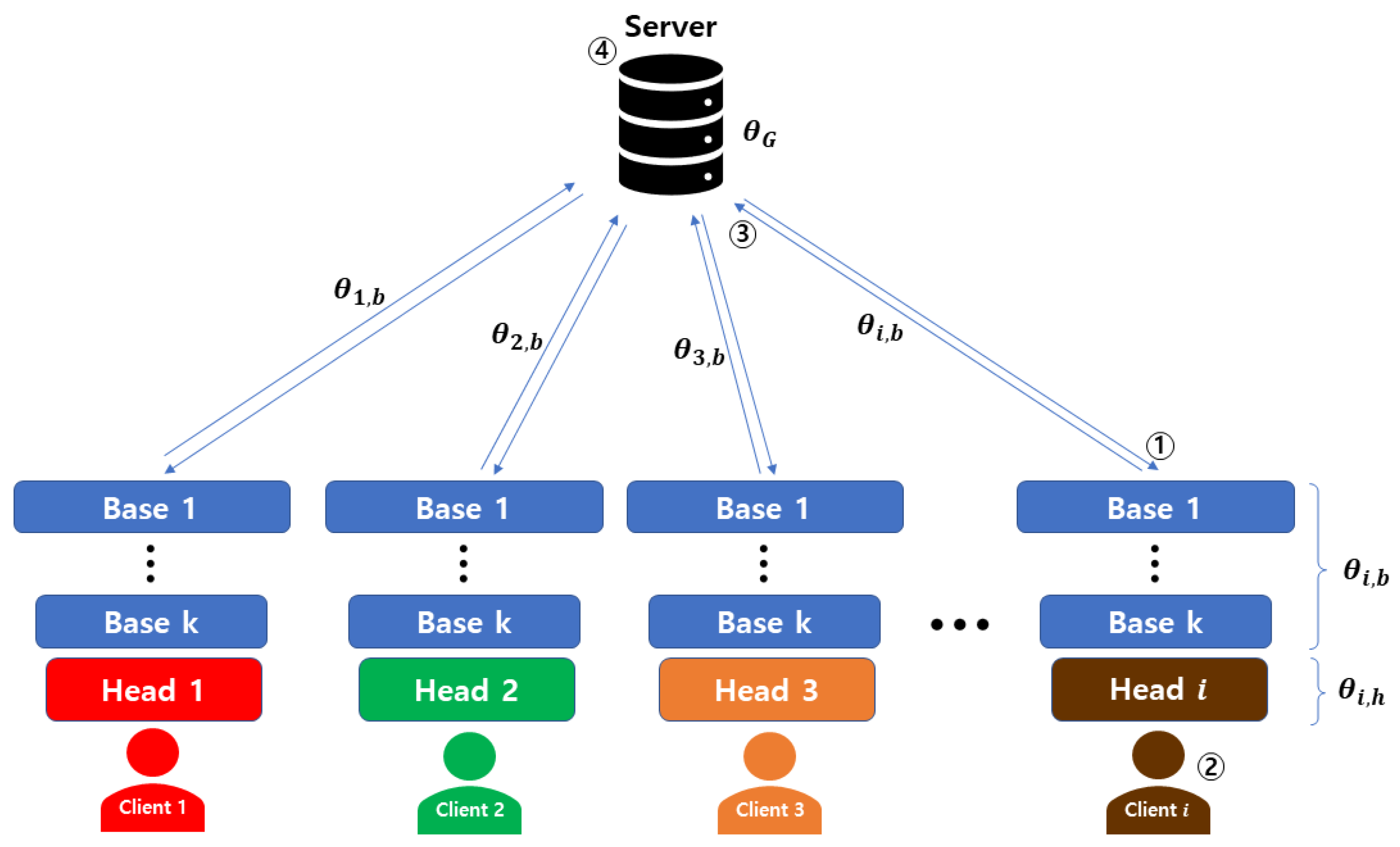
In this section, this work presents our proposed scheduling algorithms in detail, namely Vanilla Scheduling and Anti Scheduling. An overview of the proposed algorithm is shown in Figure 1. The proposed algorithm executes the following steps: (1) model distribution; (2) local training via sequential layer expansion (Vanilla or Anti Scheduling); (3) update the server with the refined base parameter ${\theta }_{i,b}$; (4) aggregate global model ${\theta }_G$. Then, steps (1)–(4) are repeated up to the predefined condition. Finally, the server fine tunes with base parameter ${\theta }_{i,b}$ and head parameter ${\theta }_{i,h}$. As shown in Figure 2, Vanilla Scheduling starts by unfreezing the shallowest layers (closest to the input) and progressively moves towards deeper layers. This method allows the model to capture low-level features early in the training process, which is crucial for building a robust foundational understanding before more high-level features are introduced. Conversely, Anti Scheduling begins with the deepest layers (closest to the output) and progressively unfreezes toward the input. This approach prioritizes the learning of high-level features from the outset, which can be beneficial for complex pattern recognition tasks that depend heavily on such features.

As shown in Figure 2, the structured progression from shallow to deep layers in Vanilla Scheduling, and the reverse in Anti Scheduling, structurally differ from traditional representation learning. In traditional representation learning methods, the base and head of the model are typically trained simultaneously without specific layer prioritization. In our approach, however, each layer’s training is specifically timed and prioritized. This strategic scheduling improves the model’s ability to adapt to the varying complexities of features throughout the training process.

Furthermore, as detailed in Section 5.2, Vanilla Scheduling can achieve comparable accuracy with significantly lower computational costs in environments characterized by high data and class heterogeneity. In contrast, Anti Scheduling excels in achieving the highest accuracy in scenarios where both data and class heterogeneity are pronounced. They both follow the basic federated learning setup and the representation learning as explained below. The list of symbols used in the paper are shown in

Table 3. List of Symbols Used.

Symbol	Description
N	Total number of clients
$C_i$	Client $i\in \{1,2,\dots ,N\}$
$|D_i|$	Number of data points for client i
$\left|D\right|$	Number of data points
T	Number of global rounds
F	Number of fine-tuning rounds
K	Number of base layers
$t_k$	Unfreeze point (round) of k-th layer
$\eta$	Learning rate
$\mathcal{L}$	Loss function
${\theta }_i$	Local parameter for client i
${\theta }_G$	Global model parameter
${\theta }_{i,b}$	Base parameter shared among all clients
${\theta }_{i,h}$	Head parameter of client i

.

As a basic federated learning setup, this work assumes that each client $C_i$ possesses data $D_i=(x_i,y_i)\in R^d$, where $i\in \{1,2,\dots ,N\}$ represents i-th client out of a total of N clients and d represents the input dimension. Each client i updates its local model parameter ${\theta }_i$ based on its data $D_i$ and the global model parameter ${\theta }_G$ as

$${\theta }_i^{(t+1)}={\theta }_i^{\left(t\right)}-\eta {\nabla }_{{\theta }_i}\mathcal{L}(D_i,{\theta }_i^{\left(t\right)}),$$

(1)

where $\eta$ is the learning rate, $\nabla L$ is the gradient of the loss function L, and $t=1,2,\dots ,T$ denotes the number of rounds. The central server updates the global parameter ${\theta }_G$ based on all clients’ local parameter updates as

$${\theta }_G^{(t+1)}=\sum _{i=1}^N{\displaystyle \frac{|D_i|}{\left|D\right|}}{\theta }_i^{(t+1)},$$

(2)

where $|D_i|$ is the number of data points for client i, and $\left|D\right|$ is the total number of data points.

For representation learning, the model parameters are divided into two components ${\theta }_i=({\theta }_{i,b},{\theta }_{i,h})$. Here, ${\theta }_{i,b}$ represents the base parameter shared among all clients, and ${\theta }_{i,h}$ represents the head parameter of the i-th client. The model parameters from Equation (1) are modified as follows:

$${\theta }_i^{(t+1)}={\theta }_i^{\left(t\right)}-\eta {\nabla }_{{\theta }_i}\mathcal{L}(D_i,{\theta }_{i,b}^{\left(t\right)},{\theta }_{i,h}^{\left(0\right)}).$$

(3)

Excluding FedBABU [20], previous works stop the gradient of the head parameter during training and during the aggregation phase. The global model is updated using both the base and head parameters. However, FedBABU and our scheduling algorithm perform both training and aggregation using only the base without involving the head. Only after training are a few rounds of fine-tuning included using both the base and head.

The aggregation process, which excludes the use of the head, proceeds as follows:

$${\theta }_G^{(t+1)}=\sum _{i=1}^N{\displaystyle \frac{|D_i|}{\left|D\right|}}{\theta }_{i,b}^{(t+1)}.$$

(4)

Our FedSeq algorithm follows the same training setup as FedBABU [20], wherein the head layer is not trained or aggregated during training; instead, it is fine-tuned for each client after training completion. In FedBABU, the training round sets the learning rate of the head to zero, allowing gradient computation but preventing its application. In contrast, our scheduling algorithm ensures complete decoupling by freezing gradients in both the head and base parts, preventing both computation and application.

3.1. Method 1: Vanilla Scheduling

Vanilla Scheduling is a training method that starts by thoroughly learning the shallowest layers (closest to the input) in the base layer, freezing the rest layers, and then progressively unfreezing them. This enables the model to preferentially learn low-level features and patterns, aiding in better understanding the abstract characteristics and patterns of the data. The training steps of Vanilla Scheduling, which starts with the shallowest layers, can be represented as

$$\begin{array}{cc}\hfill {\theta }_i^{(t_1+1)}={\theta }_i^{\left(t_1\right)}-\eta {\nabla }_{{\theta }_i}\mathcal{L}(D_i,& {\theta }_{i,b_1}^{\left(t_1\right)},{\theta }_{i,b_2}^{\left(0\right)},\dots ,{\theta }_{i,b_{K-1}}^{\left(0\right)},{\theta }_{i,b_K}^{\left(0\right)},{\theta }_{i,h}^{\left(0\right)}),\hfill \\ \hfill {\theta }_i^{(t_2+1)}={\theta }_i^{\left(t_2\right)}-\eta {\nabla }_{{\theta }_i}\mathcal{L}(D_i,& {\theta }_{i,b_1}^{\left(t_2\right)},{\theta }_{i,b_2}^{\left(t_2\right)},\dots ,{\theta }_{i,b_{K-1}}^{\left(0\right)},{\theta }_{i,b_K}^{\left(0\right)},{\theta }_{i,h}^{\left(0\right)}),\hfill \\ \hfill & ⋮\hfill \\ \hfill {\theta }_i^{(t_K+1)}={\theta }_i^{\left(t_K\right)}-\eta {\nabla }_{{\theta }_i}\mathcal{L}(D_i,& {\theta }_{i,b_1}^{\left(t_K\right)},{\theta }_{i,b_2}^{\left(t_K\right)},\dots ,{\theta }_{i,b_{K-1}}^{\left(t_L\right)},{\theta }_{i,b_K}^{\left(t_K\right)},{\theta }_{i,h}^{\left(0\right)}),\hfill \end{array}$$

(5)

where $\{t_1,t_2,\dots ,t_K\in T\}$ represent the global rounds where the freeze of each layer is released. Once the first base layer ${\theta }_{i,b_1}$ is sufficiently trained, the freeze on the next base layer ${\theta }_{i,b_2}$ is released for training. This sequential unfreezing and training of base layers up to ${\theta }_{i,b_K}$ defines Vanilla Scheduling. Throughout the training process, the head layer ${\theta }_{i,h}$ is initialized and kept frozen, only being utilized in the final fine-tuning stage.

3.2. Method 2: Anti Scheduling

Anti Scheduling is a training approach that initiates in the deepest layers (closest to the output) in the base layer, freezing the remaining layers and  progressively unfreezing them for sufficient training. This method allows the model to preferentially grasp high-level and various features. The training steps of Anti Scheduling, starting with the deepest layers, can be given as

$$\begin{array}{cc}\hfill {\theta }_i^{(t_1+1)}={\theta }_i^{\left(t_1\right)}-\eta {\nabla }_{{\theta }_i}\mathcal{L}(D_i,& {\theta }_{i,b_1}^{\left(0\right)},{\theta }_{i,b_2}^{\left(0\right)},\dots ,{\theta }_{i,b_{K-1}}^{\left(0\right)},{\theta }_{i,b_K}^{\left(t_1\right)},{\theta }_{i,h}^{\left(0\right)}),\hfill \\ \hfill {\theta }_i^{(t_2+1)}={\theta }_i^{\left(t_2\right)}-\eta {\nabla }_{{\theta }_i}\mathcal{L}(D_i,& {\theta }_{i,b_1}^{\left(0\right)},{\theta }_{i,b_2}^{\left(0\right)},\dots ,{\theta }_{i,b_{K-1}}^{\left(t_2\right)},{\theta }_{i,b_K}^{\left(t_2\right)},{\theta }_{i,h}^{\left(0\right)}),\hfill \\ \hfill & ⋮\hfill \\ \hfill {\theta }_i^{(t_K+1)}={\theta }_i^{\left(t_K\right)}-\eta {\nabla }_{{\theta }_i}\mathcal{L}(D_i,& {\theta }_{i,b_1}^{\left(t_K\right)},{\theta }_{i,b_2}^{\left(t_K\right)},\dots ,{\theta }_{i,b_{K-1}}^{\left(t_K\right)},{\theta }_{i,b_K}^{\left(t_K\right)},{\theta }_{i,h}^{\left(0\right)}).\hfill \end{array}$$

(6)

Once the deepest base layer ${\theta }_{i,b_K}$ is sufficiently trained, the freeze on the preceding layer ${\theta }_{i,b_{K-1}}$ is released for training. Anti Scheduling is thus defined as the sequential unfreezing and training of base layers starting from ${\theta }_{i,b_K}$ and proceeding to the first base layer ${\theta }_{i,b_1}$. The training progresses in the reverse order of Anti Scheduling, and during this process, the head layer ${\theta }_{i,h}$ remains frozen and is only utilized in the final fine-tuning phase.

Algorithm 1 outlines the training procedure for both Vanilla and Anti Scheduling. In line 2, a subset of clients is randomly selected. Lines 4–8 describe the Vanilla Scheduling mode operation. When the Vanilla mode is selected, if the current global round t is greater than the layers unfreeze round $t_k$, as specified in line 5, the algorithm unfreezes the k-th base parameter ${\theta }_{i,b_k}$. Then, in line 8, the unfrozen base parameters are used to perform a local update.

Lines 9–13 describe the Anti Scheduling mode operations. In Anti mode, as line 10 indicates, if the current global round t exceeds the layer unfreeze round $t_k$, the algorithm unfreezes the ($K-k+1$)-th base parameter ${\theta }_{i,b_{K-k+1}}$, which is closer to the head layer. In line 13, the unfrozen base parameters are used for the local update. In lines 15–16, the head is frozen while sending the updated base parameters to the server. In line 18, global aggregation is done after local updates, and fine-tuning is done in lines 20–24, where both base and head parameters are utilized in each client after the global rounds are complete.

Algorithm 1 FedSeq: Layer Decoupling Algorithm with Vanilla and Anti Scheduling

Input: Total global rounds T, Total clients N, join ratio r, Learning rate $\eta$, Total base layers K, Fine-tuning rounds F, Scheduling mode $Mode$, Layer unfreeze rounds $t_1,t_2,\dots ,t_K$ Initialize: Global base parameters ${\theta }_{G,b_1}^{\left(0\right)},{\theta }_{G,b_2}^{\left(0\right)},\dots ,{\theta }_{G,b_K}^{\left(0\right)}$ and Global Head parameter ${\theta }_{G,h}^{\left(0\right)}$ 1: for$t=1$to T do 2:    Randomly select $M=\lfloor r\times N\rfloor$ clients 3:    for Each selected client $i=1$ to M do 4:      if $Mode=’\mathrm{Vanilla}’$ then 5:         if $t\ge t_k$ then 6:            Unfreeze ${\theta }_{i,b_k}$ 7:         end if 8:         ${\theta }_i^{(t+1)}={\theta }_i^{\left(t\right)}-\eta {\nabla }_{{\theta }_i}\mathcal{L}(D_i,{\theta }_{i,b_1}^{\left(t\right)},\dots ,{\theta }_{i,b_K}^{\left(t\right)},{\theta }_{i,h}^{\left(0\right)})$ 9:      else if $Mode=’\mathrm{Anti}’$ then 10:         if $t\ge t_k$ then 11:           Unfreeze ${\theta }_{i,b_{K-k+1}}$ 12:         end if 13:         ${\theta }_i^{(t+1)}={\theta }_i^{\left(t\right)}-\eta {\nabla }_{{\theta }_i}\mathcal{L}(D_i,{\theta }_{i,b_1}^{\left(t\right)},\dots ,{\theta }_{i,b_K}^{\left(t\right)},{\theta }_{i,h}^{\left(0\right)})$ 14:      end if 15:      Keep ${\theta }_{i,h}$ frozen 16:      Send updated base parameters ${\theta }_{i,b_1}^{(t+1)},\dots ,{\theta }_{i,b_K}^{(t+1)}$ 17:    end for 18:    Aggregate global model ${\theta }_G^{(t+1)}={\sum }_{i=1}^N{\displaystyle \frac{|D_i|}{\left|D\right|}}{\theta }_{i,b}^{(t+1)}$ 19: end for 20: for$f=1$to F do 21:    Unfreeze all layers for each client 22:    for each client $i=1$ to N do 23:       Update all parameters ${\theta }_i$ for fine tuning 24:       ${\theta }_i^{(T+f)}={\theta }_i^{(T+f-1)}-\eta {\nabla }_{{\theta }_i}\mathcal{L}(D_i,{\theta }_{i,b_1}^{(T+f-1)},\dots ,{\theta }_{i,b_K}^{(T+f-1)},{\theta }_{i,h}^{(T+f-1)})$ 25:    end for 26: end for

4. Experiments

In our experimental setup, the total number of clients N is set to 100, with each round involving a client participation ratio r of 0.1, indicating that 10 clients participate in each training round. The batch size is configured to 10, and the learning rate is set at 0.005. The datasets used in our experiments include MNIST, which consists of 70,000 grayscale images of handwritten digits (0–9) with a resolution of 28 × 28 pixels; CIFAR-10, containing 60,000 color images of size 32 × 32 pixels across 10 classes, such as airplanes, birds, and cars; CIFAR-100⁰, which is similar to CIFAR-10 but includes 60,000 images spanning 100 classes, organized into a hierarchy of 20 superclasses; and Tiny-ImageNet, a dataset consisting of 200 classes with 500 training images and 50 validation images per class, each resized to 64 × 64 pixels. To induce heterogeneity among the data distributed to each client, this work sampled from a Dirichlet distribution with a Dirichlet parameter of 0.1, establishing a highly heterogeneous environment. This approach to data distribution is visualized in Figure 3, which illustrates the results of sampling the CIFAR-10 dataset among 10 clients. Despite the high heterogeneity induced by the Dirichlet parameter $\alpha$ of 0.1, MNIST, and CIFAR-10 datasets inherently lack significant class heterogeneity. Therefore, our experiments focus on the CIFAR-100 and Tiny-ImageNet datasets because our approach performs well in environments with substantial data and class heterogeneity. The CIFAR-100 dataset contains 100 different classes, and the Tiny-ImageNet dataset contains 200 classes.

In our experiments, the proposed algorithm is compared against six baselines, as detailed in the following references: [3,16,17,18,19,20]. The model used is a CNN model comprising two convolutional layers and two fully connected layers. Here, the last fully connected layer is set as the head, and the remaining three layers are designated as the base. The total number of base layers K is set to 3, with $t_1$ at the 0 (initial) round, $t_2$ at the 100-th global round, and $t_3$ at the 200-th global round. Additionally, in FedBABU [20], the learning rate of the head is set to zero during the training rounds, implying that gradients are calculated but not applied. In contrast, our scheduling algorithm achieves complete decoupling by freezing the gradients, thus preventing both computation and application. It will delve into the comparison of computational and communication costs in Section 5.2.

Table 4. Comparison of accuracy.

Algorithm	MNIST		CIFAR-10		CIFAR-100		Tiny-ImageNet
	Acc. (%)	$\mathbf{T}$	Acc. (%)	$\mathbf{T}$	Acc. (%)	$\mathbf{T}$	Acc. (%)	$\mathbf{T}$
FedAvg [3]	91.48	100	36.87	100	29.04	500	16.97	300
	96.32	200	42.00	200	30.95	1000	14.06	500
	97.48	300	49.36	300	30.34	1500	14.27	1500
FedPer [16]	98.30	100	86.16	100	40.22	500	29.04	300
	98.63	200	87.34	200	41.03	1000	29.24	500
	98.69	300	86.66	300	40.05	1500	29.11	1000
LG-FedAvg [17]	97.95	100	85.75	100	41.06	500	26.46	300
	98.17	200	86.10	200	41.01	1000	26.35	500
	98.13	300	85.91	300	40.80	1500	26.36	1000
FedRep [18]	98.56	100	86.58	100	40.44	500	28.85	300
	98.69	200	88.12	200	41.24	1000	28.54	500
	98.75	300	88.11	300	40.66	1000	28.50	1000
FedROD [19]	98.61	100	86.24	100	49.50	500	37.23	300
	98.95	200	88.01	200	48.70	1000	35.34	500
	99.06	300	88.59	300	50.56	1500	35.35	1000
FedBABU [20]	98.19	100	85.77	100	49.28	500	37.84	300
	98.77	200	86.16	200	52.75	1000	33.78	500
	98.84	300	87.07	300	51.82	1500	32.57	1000
FedSeq (Vanilla Scheduling)	98.21	100	85.82	100	56.86	500	41.86	300
	98.84	200	87.81	200	59.52	1000	39.51	500
	98.99	300	88.58	300	58.49	1500	36.44	1000
FedSeq (Anti Scheduling)	98.34	100	85.73	100	56.17	500	41.94	300
	98.81	200	87.67	200	60.06	1000	39.67	500
	98.96	300	88.61	300	58.58	1500	36.63	1000

presents a comparison of the accuracies achieved by various federated learning algorithms across multiple datasets, including MNIST, CIFAR-10, CIFAR-100, and Tiny-ImageNet. It encompasses representation learning algorithms such as FedAvg [3], FedPer [16], LG-FedAvg [17], FedRep [18], FedROD [19], and FedBABU [20], as well as our proposed Vanilla and Anti Scheduling algorithms. While FedAvg [3] serves as the foundational algorithm in federated learning, it is not a personalized federated learning (PFL) method. Unlike PFL approaches, FedAvg updates both the base and head layers of the model uniformly across clients without personalization. In contrast, the other algorithms explored are PFL methods focused on representation learning. For instance, FedPer [16] retains personalized layers at each client while sharing a global base model. LG-FedAvg [17] decouples global and local updates to improve personalization. FedRep [18] separates model representation from the classifier to facilitate client-specific adjustments. FedROD [19] employs robust optimization to tackle client distribution heterogeneity. A key aspect of both FedBABU and our scheduling algorithms is their approach during the training phases leading up to the final global round, denoted as T. Characteristically, these algorithms exclusively use the base layers and do not employ the head layer during the training rounds, resulting in relatively lower accuracies prior to the final round. To ensure a fair comparison, the accuracy figures for FedBABU and our scheduling algorithms at T represent the performance after fine-tuning. Additionally, it is noteworthy that our scheduling algorithms have achieved high accuracy in environments with significant data and class heterogeneity, demonstrating their effectiveness in processing complex and diverse datasets.

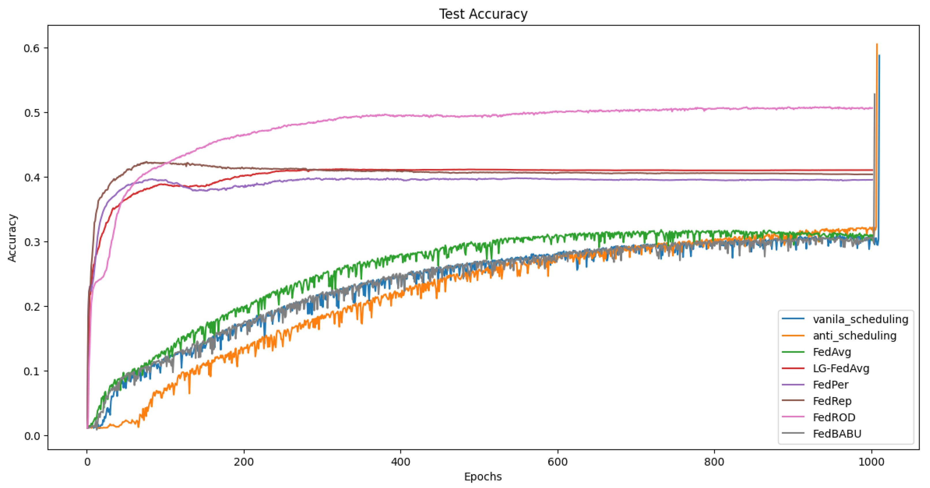
Figure 4 shows the average accuracy of clients on the CIFAR-100 dataset, visualizing the performance of our scheduling algorithms compared to baselines. As can be seen, the earlier round accuracy of our scheduling algorithm is lower than FedAvg and FedBABU, which is attributed to the fact that, in the earlier rounds, not only all base but also head is used, and the training is conducted using only a portion of the unfrozen base layers.

Similarly, Figure 5 represents the average accuracy of clients on the Tiny-ImageNet dataset. Our scheduling algorithm’s earlier round accuracy is lower than FedAvg and FedBABU, which is consistent with its characteristics. This visualization helps underscore how our scheduling algorithms gradually catch up and potentially surpass other algorithms as the training progresses.

5. Ablation Study

In our ablation study, this work demonstrates the results of varying different parameters. The contents to be covered in the ablation study include:

• Comparison of client-specific accuracy
• Estimation of computational cost for each algorithm
• Effect of layer unfreezing timing on the accuracy
• Application of scheduling to the baseline algorithms

5.1. Comparison of Client-Specific Accuracy

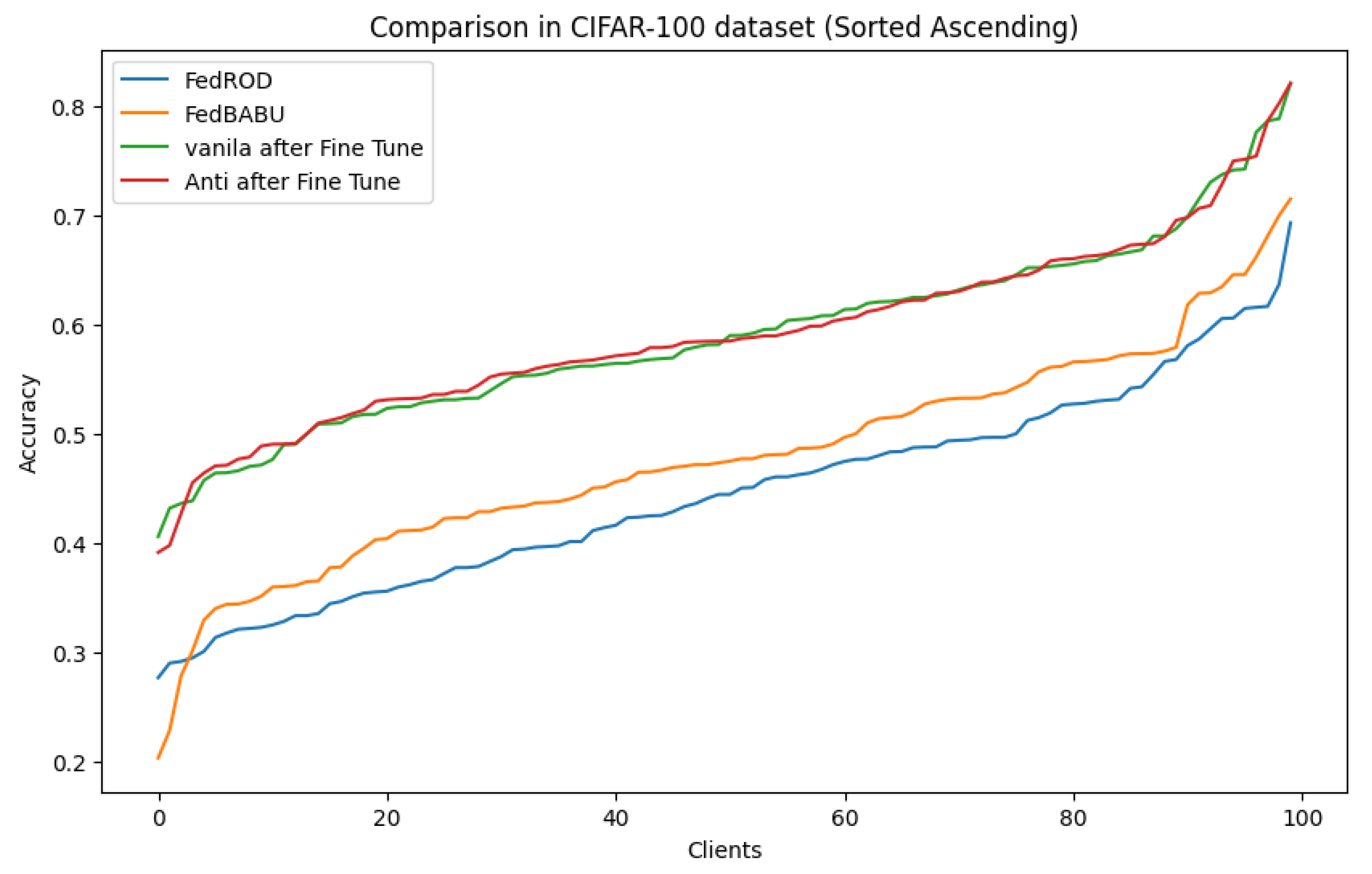
To ensure that accuracy improvements during fine-tuning are not biased or limited to specific clients, This work conducted a comparative analysis of client-specific accuracy between the latest representation learning algorithms and our algorithm. Since the accuracy differences in the MNIST and CIFAR-10 datasets are not significantly pronounced, the comparison was focused on the CIFAR-100 and Tiny-ImageNet datasets. The results demonstrated that the higher average accuracy of our scheduling algorithm was not due to bias towards specific clients but was consistently achieved across all clients.

Figure 6 shows the comparison of client-specific accuracy in the CIFAR-100 dataset. This visualization helps to highlight that our scheduling algorithm achieves consistent accuracy across a spectrum of different clients without favoring any particular group.

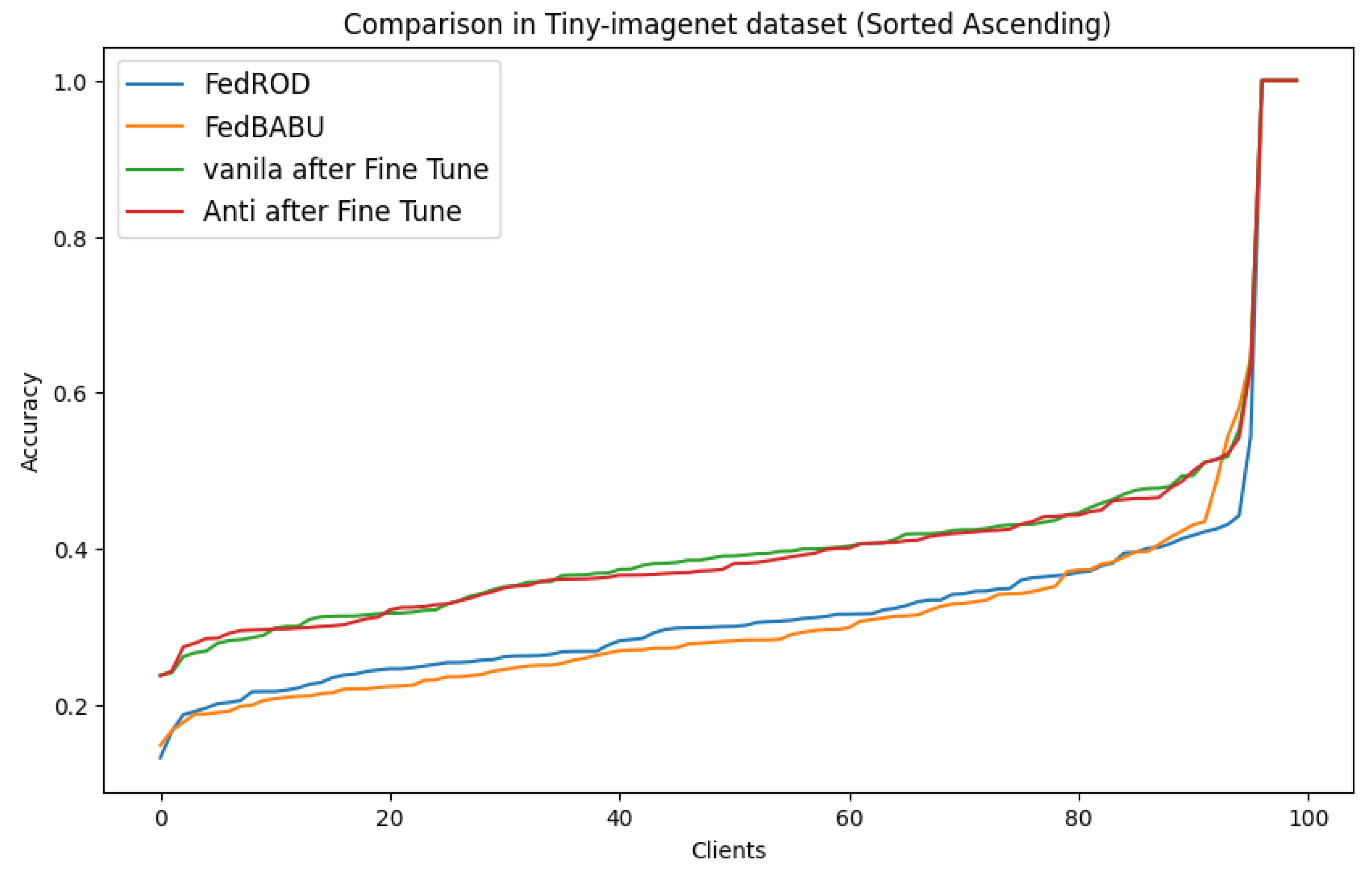
Similarly, Figure 7 demonstrates the client-specific accuracy in the Tiny-ImageNet dataset. As with CIFAR-100, the visualization confirms that our algorithm manages to maintain high accuracy uniformly across different clients, showcasing its robustness.

5.2. Estimation of Computational Cost for Each Algorithm

In the actual experimental environment, using non-IID data makes it challenging to estimate computational costs. Therefore, this work estimates the computational costs using the number of FLOPs. The number of parameters in each layer is mentioned in

Table 5. Number of parameters per layer.

Layer	Number of Parameters
conv1.weight	800
conv1.bias	32
conv2.weight	51,200
conv2.bias	64
fc1.weight	524,288
fc1.bias	512
fc2.weight	5120
fc2.bias	10
Total	582,026

.

To compare the computational costs of FedAvg, FedBABU, and our scheduling algorithms, this work considers the data processed by each client in an IID (independent and identically distributed) environment. Costs are measured in FLOPs, and for simplicity, all algorithms are assumed to use datasets with an equal pixel count per image. In datasets like MNIST, CIFAR-10, and CIFAR-100, each with a total of 50,000 training data points and 100 clients, each client processes 500 data points. In the setting of our experiments, a batch size of 10 is used, with each client handling 50 batches per epoch.

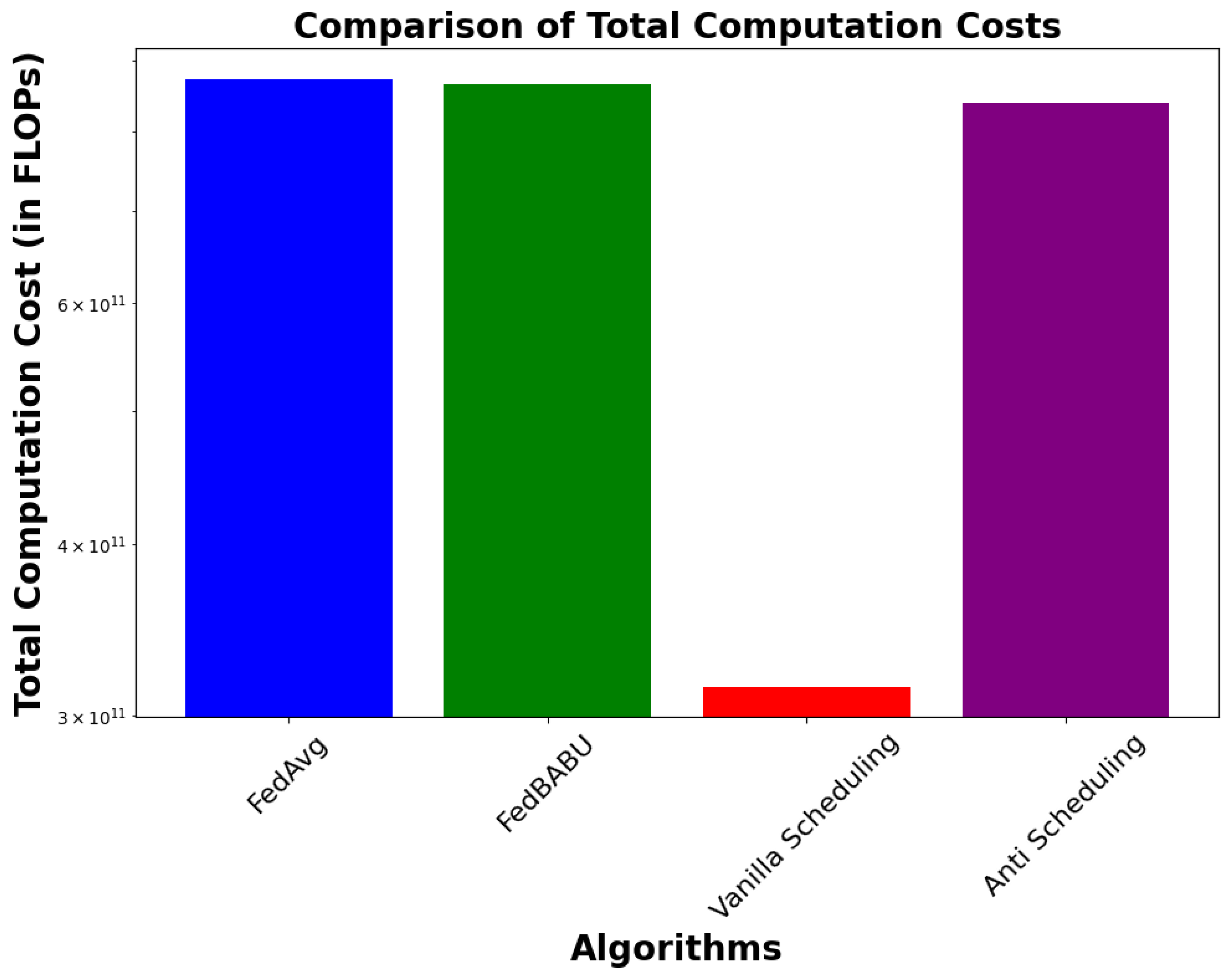
For FedAvg, as seen in Table 5, the total model parameters are 582,026, and the computational cost per round is 582,026 × 50. Thus, the total computational cost for all clients and all rounds is 873.039 billion FLOPs. In the same environment, the computational cost for FedBABU, considering that the head (fc2) layer parameters are not computed during the training rounds, results in 576,896 learning parameters. Hence, the total computational cost for FedBABU is 865.344 billion FLOPs. Using the same method for our scheduling algorithms, the computed parameters result in 314.912 billion FLOPs for Vanilla Scheduling and 838.880 billion FLOPs for Anti Scheduling, as detailed in

Table 6. Comparison of Computational Cost.

Algorithm	Number of FLOPs $(\times {10}^9)$	T
FedAvg [3]	873.04	300
FedBABU [20]	865.34	300
Vanilla Scheduling	314.91	300
Anti Scheduling	838.88	300

.

Figure 8 visually compares the computational costs between FedAvg, FedBABU, and our scheduling algorithms. It illustrates how Vanilla Scheduling significantly reduces computational costs in the earlier rounds by updating only the earlier unfreezed layers. This visualization supports the data presented in Table 6, emphasizing the efficiency of Vanilla Scheduling in managing computational resources.

5.3. Accuracy Differences Due to Changes in Layer Unfreezing Timing

In our two scheduling algorithms, the number of base layers, $t_k$, is set to 3, leading to parameter unfreezing occurring across three phases. For instance, in Vanilla Scheduling, training proceeds with the unfreezing of the conv1 layer from round $T=0$ to 100. Subsequently, from rounds 100 to 200, both conv1 and conv2 layers are unfrozen for training. Finally, from round 200 to the final global round, all base layers, including conv1, conv2, and fc1, are unfrozen and utilized for training. While the unfreezing points in this paper are arbitrarily set for discussing the effectiveness of layer decoupling, an appropriate scheduling method is required accordingly. Therefore, this work compares the differences in outcomes when unfreezing occurs at rounds 50 and 100 instead of 100 and 200.

In the CIFAR-100 dataset, with the global round $T=1000$ and layer unfreezing round set at $t_1=0,\hspace{0.17em}{t}_2=100,\hspace{0.17em}{t}_3=200$, Vanilla Scheduling achieves an accuracy of 59.52%, while Anti Scheduling achieves 60.06%. However, when the unfreezing round is changed to $t_1=0,\hspace{0.17em}{t}_2=50,\hspace{0.17em}{t}_3=100$, Vanilla Scheduling achieves 58.68%, and Anti Scheduling achieves 59.02% accuracy, slightly lower accuracy. For the Tiny-ImageNet dataset at global round $T=300$, with $t_1=0,\hspace{0.17em}{t}_2=100,\hspace{0.17em}{t}_3=200$, Vanilla and Anti Scheduling achieve accuracies of 41.86% and 41.94%, respectively. Changing the unfreezing points to $t_1=0,\hspace{0.17em}{t}_2=50,\hspace{0.17em}{t}_3=100$ results in accuracies of 41.23% for Vanilla and 41.63% for Anti Scheduling, which are also slightly lower. The insight gained here is that while the timing of layer unfreezing does not significantly affect accuracy, as seen in Section 5.2, it has a substantial impact on computational cost. Therefore, setting larger values for $t_k$ is advantageous where possible.

5.4. Application of Scheduling to Baseline Algorithms

When our scheduling methods were applied to the baseline algorithms, no noticeable improvement was observed in accuracy. This is attributed to the fact that, except for [20], other algorithms update the head during training rounds, which nullifies the effect of freezing base layers. Furthermore, Vanilla Scheduling achieved a performance similar to the non-scheduled approach, while Anti Scheduling, in particular, resulted in significantly lower accuracy. Therefore, naively applying a dense division of the base layer only for scheduling purposes might inadvertently lead to a negative impact on accuracy. Additionally, if the head layer is utilized for local updates during training, the intended effect of freezing the base layers is effectively nullified.

6. Conclusions

This research introduces a layer decoupling technique in representation learning, a domain of personalized federated learning, to address data and class heterogeneity among clients. In traditional representation learning, the model is divided into ‘base’ and ‘head’ components, each customized to process the common and unique features of client data, respectively. Our primary contribution focuses on the dense division of the base component in representation learning and the subsequent application of two novel scheduling methodologies, namely Vanilla and Anti Scheduling, to these finely segmented base layers in federated learning architecture. The Vanilla Scheduling approach excels in significantly reducing computational costs without degrading model performance. This aspect is particularly crucial in federated learning environments where resources and computational power are often limited. Conversely, Anti Scheduling demonstrates superior capability in handling scenarios with pronounced data and class heterogeneity. Our experimental analysis, conducted on datasets with high data and class heterogeneity, such as CIFAR-100 and Tiny-ImageNet, shows that these scheduling methods not only contribute to a more efficient training process but also ensure fair improvements in accuracy across all clients. This addresses the challenges of personalized federated learning by ensuring that no single client’s data disproportionately influences the global model.

7. Privacy Considerations and Future Work

While federated learning is designed to enhance privacy by keeping raw data on local devices, recent studies such as ‘Deep Leakage from Gradients [23]’ and ‘Inverting Gradients [24]’ have revealed that private information can still be reconstructed from shared model gradients, posing potential privacy risks. Our approach may offer an inherent privacy advantage by limiting the number of base layers actively involved in model updates, thus reducing the amount of sensitive information exposed through gradients. However, to further strengthen privacy protection, future work will explore integrating advanced privacy-preserving techniques, such as differential privacy and secure aggregation, into our framework.

Additionally, Future work will involve visualizing the characteristics of each layer at every global round to track changes as training progresses. This approach is expected to facilitate the introduction of more sophisticated scheduling mechanisms that can reflect the unique data characteristics of clients in heterogeneous environments, thereby enhancing learning efficiency. Dynamic scheduling techniques will also be developed to enable rapid adaptation to new data. Additionally, future work will focus on exploring the trade-off between computational cost and learning accuracy by adjusting the layers involved in training. Furthermore, it will extend to how decoupling techniques can be applied to more complex architectures, such as RNN or Transformer models.